Design and Analysis of High-Accuracy Telecentric Surface Reconstruction System Based on Line Laser

Abstract

Non-contact measurement technology based on triangulation with cameras is extensively applied to the development of computer vision. However, the accuracy of the technology is generally not satisfactory enough. The application of telecentric lenses can significantly improve the accuracy, but the view of telecentric lenses is limited due to their structure. To address these challenges, a telecentric surface reconstruction system is designed for surface detection, which consists of a single camera with a telecentric lens, line laser generator and one-dimensional displacement platform. The designed system can reconstruct the surface with high accuracy. The measured region is expanded with the used of the displacement platform. To achieve high-accuracy surface reconstruction, we propose a method based on a checkerboard to calibrate the designed system, including line laser plane and motor direction of the displacement platform. Based on the calibrated system, the object under the line laser is measured, and the results of lines are assembled to make the final surface reconstruction. The results show that the designed system can reconstruct a region of $20\times 40 {\mathrm{mm}}^2$, up to the accuracy of micron order.

1. Introduction

Due to the significant advance in optical electronic technology, micro-electronic technology and industrial manufacturing, non-contact measurement technology based on triangulation with cameras has come to the foreground [1]. Compared with other measured technology, non-contact measurement based on triangulation with cameras is commercial and fast when there is not a strict requirement for accuracy. The perspective effect and lens distortion of conventional lenses affect the accuracy severely in close-range measurement [2]. However, the application of telecentric lenses further elevates the accuracy for non-contact measurement with cameras, especially for the 3D metrology in a microscopic scale, since telecentric lenses provide the orthographic projection and possess the characteristics of low distortion, constant magnification and amplified depth of field [3,4,5]. As it is different from conventional lenses for telecentric lenses in imaging models and calibration methods, the research about non-contact measurement with telecentric lenses has become one of the hotspots in this field recently [6,7].

Analogously, telecentric non-contact measurement technology can also be divided into active and passive techniques. Passive techniques do not rely on an external light source while active techniques are quite the contrary. Among passive techniques, telecentric stereo vision is on the forefront [8,9,10]. Compared with passive techniques, active techniques are highly applied for better performance in accuracy. The light sources employed in active techniques mainly contain structured light and laser light [11]. For the techniques of structured light, it is the combination of the projector and camera. There has been research which employs the projector with a conventional lens and the camera with a telecentric lens, respectively, and also the projector and camera both staffed with telecentric lens [12]. Moreover, the light system of binocular cameras with telecentric lenses is studied [13,14]. The techniques of structured light need to project several structured light images to measure a narrow invariant region. Meanwhile, the techniques of laser light, also called laser scanner techniques, generally require a single camera, a laser generator and a platform [15]. The measured range of laser scanner techniques is determined by the platform employed, among which a 1D displacement platform is frequently utilized in industrial inspection [16], while other types of platforms are used for 3D reconstruction and other applications [17,18]. The adoption of telecentric lens has become the tendency to improve the accuracy for techniques of laser light.

In order to realize the high-accuracy measurement with the techniques of laser light with telecentric lenses, there are three main challenges. The first challenge is the unmeasured region caused by the principle of triangulation. The technique is essentially based on the intersection of the optical line and laser plane, which leads to a systematic error when the surface of the measured object is abrupt enough [19]. The intersection angle forms an unmeasured region due to occlusion where depth changes significantly. The second challenge is that the calibration method for conventional lenses is not suitable for telecentric lenses due to their different projection model [20]. Moreover, the recovery of the depth information for telecentric lens is not direct, and the problem also affects the system structure calibration for the system with telecentric lenses. The last challenge is the laser stripe extraction. The laser stripe in image is expected to be an ideal line without width. Nevertheless, it is too wide to be used for positioning directly in practice, so a sub-pixel laser stripe extraction method is essential and it can directly affect the measured accuracy [16].

In this paper, a high-accuracy surface reconstruction system is established with telecentric lenses, a line laser generator and 1D displacement platform, which can be mainly applied in a circuit board test, surface roughness measurement, flatness measurement and other industrial inspections. The main contributions of the work are listed as follows. (1) Theoretical analysis is proposed to analyze the systematic error for the triangulation with a line laser, and the result of the analysis guides the system parameters selected for certain applications. (2) A gray scale-weighted centroid algorithm is proposed to realize the sub-pixel location of the laser line to obtain the center line for the laser line in the practical image. (3) A telecentric intersection process is presented only with the knowledge of the normal direction of the laser plane, and the intersection results are transferred into a global coordinate system with the motor direction of the displacement platform.

The principal part of the paper is organized as noted below. At first, the design of the system is introduced in Section 2, in which the systematic error based on the design is analyzed. Next, a complete calibration procedure is presented for the telecentric surface metrology system in Section 3, including the single camera calibration and the calibration of system structure parameters. Then, this is followed by the measurement procedure in Section 4, in which a weighted centroid algorithm based on gray scale is used to achieve laser stripe extraction, and the telecentric intersection process is presented. At last, experiments are presented to indicate the performance of the system in Section 5, and the evaluation of uncertainty is analyzed. Some concrete applications of surface detecting are realized in the experiments part, including defect detecting and circuit board tests.

2. System Design

The telecentric surface metrology system in this study is designed for the measurement of micro-scale surfaces, such as industrial inspection for circuit boards. The system consists of a single camera with a telecentric lens, a micro line laser generator and a one-dimensional (1D) displacement platform. As shown in Figure 1, all components are completely fixed on a workbench to reduce the measurement uncertainty. During the measurement procedure, the object measured is fixed on the motor desk of the displacement platform. The precise movement of the desk along the guideway leads to the relative movement between the object and laser, which realizes the linear pushbroom imaging for the measured surface. To achieve the measurement, the single telecentric camera is supposed to be calibrated, and the location of line laser plane and the motor direction of the motor desk in the world coordinate system are required. Hence, these issues are studied and proposed in Section 3.

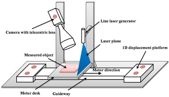
Figure 1. Telecentric surface metrology system based on laser scanning.

2.1. Systematic Error Analysis

Due to the measurement principle of the intersection of the optical line and laser plane, the systematic error in this system is inevitable. The point on the object surface is located only if the point is lighted up by the laser while it is captured by camera. Nevertheless, as there must be an intersection angle between the optical axis of camera and the laser plane, a blind corner is formed for the camera when the surface of the measured object is abrupt enough. As it is shown in Figure 2, suppose the laser plane is perpendicular to the motor direction of the measured object, when the intersection angle is α, and the depth difference on the object surface is $H$, the width of blind corner $D$ is expressed as

$$D=H\cdot \mathbf{tan}\alpha .$$

(1)

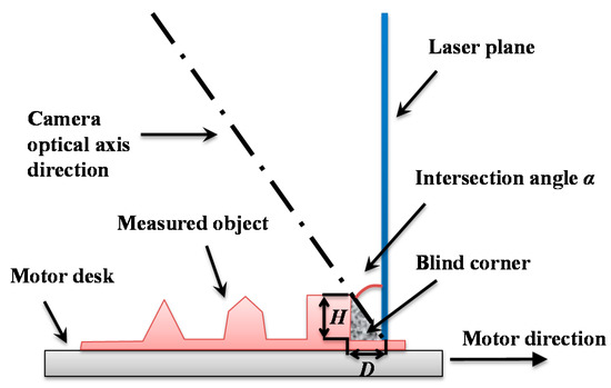
Figure 2. Formation mechanism of the blind corner.

Figure 2 indicates that the shaded region along the movement direction is not able to be measured. The region area is characterized by the width $D$ directly when $H$ is constant. Intuitively, the smaller $\alpha$ reflects the narrower $D$ within $\alpha \in \left(0°, 90°\right)$. Nevertheless, the resolution of the surface depth is positively associated with the intersection angle $\alpha$ for $\alpha \in \left(0°, 90°\right)$. The description can be found in Figure 3, according to the telecentric camera model, which is presented in Section 3, the resolution $r$ can be formulated as

$$r=\frac{\Delta u}{\Delta H}=\frac{M}{\delta u}\cdot \mathbf{sin}\alpha .$$

(2)

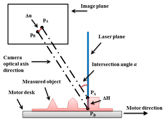
Figure 3. The resolution analysis in depth direction.

$M$ is the magnification of telecentric lens, and $\delta u$ is the cell size of the camera sensor. The resolution $r$ represents image pixels corresponding to unit surface depth. For instance, if the recognized depth required is $h$, it is supposed that Equation (3) should be satisfied. Note that the $h$ discussed here cannot be microcosmic due to the diffraction limit for optical imaging.

$$h\cdot r\ge \mathsf{\Delta }p,$$

(3)

$\mathsf{\Delta }p$ is the minimum of distinguishable pixel difference, and it can be set to 0.5 pixel, while it has to be larger considering the noise aspect and other random errors. Compare the derivative of the trigonometric part of Equations (1) and (2), which are $\tan \prime \alpha =1/{\cos }^2\alpha$ and $\sin \prime \alpha =\cos \alpha$/The variation tendency is presented in Figure 4.

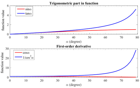
Figure 4. The variation tendency for the trigonometric part.

It is indicated that both $\tan \alpha$ and $\sin \alpha$ increase within $\alpha \in \left(0°, 90°\right)$, but $\tan \alpha$ climbs much faster than $\sin \alpha$, especially for $\alpha >60°$. Hence, the intersection angle is generally no more than $60°$ in surface metrology. As there is a contradiction for the intersection angle $\alpha$ chosen, the system design must combine equipment condition with concrete demand of the applications in practice. Hence, an actual system is established for circuit boards tests as an instance.

2.2. System Establishment for Circuit Boards Test

As it is analyzed for system design, an actual system is carried out for circuit boards tests. As far as it is concerned, the surface depth difference of circuit board is from 50 to 100 $\mathsf{\mu }\mathrm{m}$ in general. The camera and telecentric lens employed in the system are IGV-B2520M, Imperx, Boca Raton, Florida 33487, USA (resolution: 2456 $\times$ 2058; sensor size: $2/3″$; cell size: 3.45 $\mathsf{\mu }\mathrm{m}$) and DTCM430-56-AL, COOLENS, Shenzhen 518000, Guangdong, China (magnification: 0.429), respectively. The laser module is EL405-20GXLP, ELITE, Xi’an 710000, Shanxi, China (wavelength: 405 $\mathrm{nm}$; line width: 20 $\mathsf{\mu }\mathrm{m}$) while the 1D displacement platform is M-511.DG1 with C863.11, PI, Karlsruhe 76228, Germany (travel range: 102$\mathrm{mm}$; design resolution: 0.033 $\mathsf{\mu }\mathrm{m}$).

According to the equipment and application requirement, the intersection angle can be determined. On one hand, the error of measured surface depth is expected to be less than 10 $\mathsf{\mu }\mathrm{m}$, which means $h$ is set to be 10 $\mathsf{\mu }\mathrm{m}$. It is obtained that the intersection angle is $\alpha \ge 23.7°$ from Equation (3) while $\mathsf{\Delta }p$ is set to 0.5 pixel. On the other hand, the width of the blind corner is expected to be as narrow as possible. In order to keep more details under satisfying the precondition of functional demands, the intersection angle $\alpha$ designed is finally set to $30°$.

3. System Calibration

The calibration is the fundamental step in metrology. It recovers the metrology information and makes the devices work as a system. For the designed system, the calibration contains single camera calibration, laser plane calibration and motor direction calibration. The single camera calibration calculates the camera parameters. Laser plane calibration calculates the normal direction of the laser plane in the world coordinate system. Motor direction calibration calculates the displacement direction of the vector of the motor desk in the world coordinate system. Laser plane calibration and motor direction calibration are collectively called system structure parameter calibration. In this system, we simply regard the camera coordinate system as the world coordinate system. The camera parameters and the normal direction of the line laser plane are used to achieve intersection of the measurement with images of the measured object, while the motor direction of the platform is used to mosaic the intersection results.

3.1. Single Camera Calibration

For the calibration of a single camera with a telecentric lens, we have proposed a flexible calibration approach in [20]. According to the description, the distortion-free telecentric camera model is expressed as

$$\left[\begin{array}{c}u\\ v\\ 1\end{array}\right]=\left[\begin{array}{c}M/d_u \\ 0\\ 0\end{array} \begin{array}{c}0\\ M/d_v \\ 0\end{array} \begin{array}{c}0\\ 0\\ 0\end{array} \begin{array}{c}{u}_0\\ v_0\\ 1\end{array}\right]\left[\begin{array}{c}{x}_c\\ y_c\\ z_c\\ 1\end{array}\right]=\left[\begin{array}{c}M/d_u \\ 0\\ 0\end{array} \begin{array}{c}0\\ M/d_v \\ 0\end{array} \begin{array}{c}0\\ 0\\ 0\end{array} \begin{array}{c}{u}_0\\ v_0\\ 1\end{array}\right]\left[\begin{array}{cc}R& t\\ 0_{1\times 3}& 1\end{array}\right]\left[\begin{array}{c}{x}_w\\ y_w\\ z_w\\ 1\end{array}\right],$$

(4)

where $\left(x_w,y_w,z_w\right)$ and $\left(x_c,y_c,z_c\right)$ are the 3D coordinates of the object point $P$ in the world coordinate system and camera coordinate system, respectively. $\left(u,v\right)$ is the image coordinate of $P$ in pixels. $M$ is the effective magnification of the telecentric lens, and $\left(u_0,v_0\right)$ is the coordinate of the image plane center. $d_u$ and $d_v$ denote the cell size in $u$ and $v$ directions for the camera, respectively. Generally, it is defined that $m=M/d_u=M/d_v$ when $d_u$ and $d_v$ are the same for a sensor. Equation (4) can be rewritten as follows, in which $R_s$ is the upper left $2\times 2$ sub-matrix of $R$ while $t_s$ is the first two truncated translations of $t$.

$$\left[\begin{array}{c}u\\ v\\ 1\end{array}\right]=\left[\begin{array}{ccc}m& 0& u_0\\ 0& m& v_0\\ 0& 0& 1\end{array}\right]\left[\begin{array}{c}{x}_c\\ y_c\\ 1\end{array}\right]=K\left[\begin{array}{cc}{R}_s& t_s\\ 0_{1\times 2}& 1\end{array}\right]\left[\begin{array}{c}{x}_w\\ y_w\\ 1\end{array}\right].$$

(5)

The calibration method mentioned is a two-step procedure with a coded calibration board. In the first step, camera parameters with a distortion-free telecentric camera model are achieved by a closed-form solution, which is solved from a homographic matrix. In the second step, a non-linear optimization is performed to refine the coordinates of control points with distortion-free camera parameters, and follows another non-linear optimization for all the camera parameters including the distortion coefficients and distortion center.

In this way, the camera calibration parameters are achieved. The calibration results contain effective magnification $M$, and extrinsic parameters for each calibration image $\left(R_i,t_{si}\right)$. Note that the rotation matrix $R_i$ is completed while $t_{si}={\left(t_{xi},t_{yi}\right)}^T$ is the truncated translation.

3.2. Laser Plane Calibration

Laser plane calibration determines the normal direction of the line laser plane in the camera coordinate system. Inspired by [21], the calibration method for laser plane calibration is developed. The principle of the method is first to calculate several laser lines in the camera coordinate system by plane intersection as shown in Figure 5, and then the normal direction of the laser plane can be determined by the several laser lines. The concrete calibration procedure is as follows.

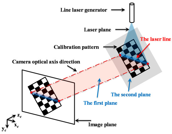
Figure 5. Two planes across the laser line.

Actually, the calibration images used in this step are also the images used in single camera calibration. For the i-th calibration image, the line laser illuminated on the plane pattern is regarded as a line in the image, which can be expressed as

$$a_{i}u+b_{i}v+c_i=0$$

(6)

Combining Equations (5) and (6), as it is shown in Figure 5, the first plane across the laser line can be expressed as Equation (7) in the camera coordinate system.

$$a_{i}m\cdot x_c+b_{i}m\cdot y_c+a_i{u}_0+b_i{v}_0+c_i=0$$

(7)

The unit normal vector of the plane in Equation (7) is ${\left(a_i/\sqrt{a_i^2+b_i^2},b_i/\sqrt{a_i^2+b_i^2},0\right)}^T$. Meanwhile, the calibration board is the second plane across the laser line. The unit normal vector of the plane in the camera coordinate system is ${\left(r_{13-i},r_{23-i},r_{33-i}\right)}^T$, which is the third column of the corresponding rotation matrix $R_i$ achieved in single camera calibration. Therefore, the unit vector of the laser line on the $i^{th}$ calibration image can be obtained by the unit normal vectors of the above two planes.

$$n_{li}={\left(\frac{a_i}{\sqrt{a_i^2+b_i^2}},\frac{b_i}{\sqrt{a_i^2+b_i^2}},0\right)}^T\times {\left(r_{13-i},r_{23-i},r_{33-i}\right)}^T.$$

(8)

With Equation (8), a unit vector is determined for every calibration image in the camera coordinate system. Meanwhile, the corresponding laser lines of the unit vectors are located in the laser plane, and the normal vector of the laser plane can be recovered with at least two unit vectors ideally which are not parallel. In practice, more direction vectors are placed to overcome the impact of noise. The unit normal vector of the laser plane $n_p$ can be obtained by minimizing the following formula with the Singular Value Decomposition (SVD) method.

$$\min {{\displaystyle \sum }}_{i=1}^m\Vert n_{li}^T{n}_p\Vert {}^2, \mathrm{subject} \mathrm{to} \left|n_p\right|=1.$$

(9)

3.3. Motor Direction Calibration

The motor direction of the 1D displacement platform in camera coordinate system is another system structure parameter required, which is described in Figure 6. The calibration procedure is realized by fixing a calibration board on the motor desk of the displacement platform, and controlling the desk to move a certain distance. The camera is used to obtain the image capture before and after the movement, respectively.

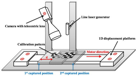
Figure 6. Motor directions calibrated in structure calibration.

Let $P_{j1}={\left(x_{cj1},y_{cj1},z_{cj1}\right)}^T$ and $P_{j2}={\left(x_{cj2},y_{cj2},z_{cj2}\right)}^T$ be the corresponding coordinates of the control points before and after the movement in the camera coordinate system, respectively, in which $j$ is the count of the control points. From Equation (5), ($x_{cj1},y_{cj1}$) and ($x_{cj2},y_{cj2}$) can be determined by the corresponding image coordinates $\left(u_{j1},v_{j1}\right)$ and $\left(u_{j2},v_{j2}\right)$. Meanwhile, the certain distance $d$ of $P_{j1}{P}_{j2}$ is obtained from the displacement platform.

$$d=\Vert P_{j1}{P}_{j2}\Vert =\sqrt{{\left(x_{cj1}-x_{cj2}\right)}^2+{\left(y_{cj1}-y_{cj2}\right)}^2+{\left(z_{cj1}-z_{cj2}\right)}^2}.$$

(10)

Thus, the displacement on the $Z_C$ axis is achieved, and the sign ambiguity can be avoided with the distribution of the camera and displacement platform. Suppose $z_{cj1}<z_{cj2}$, then the unit motor direction of the displacement platform $n_d$ in the camera coordinate system is expressed in Equation (11).

$$n_d=\frac{\overrightarrow{P_{j1}{P}_{j2}}}{\Vert P_{j1}{P}_{j2}\Vert }={\left(\frac{x_{cj2}-x_{cj2}}{d},\frac{y_{cj2}-y_{cj2}}{d},\frac{\sqrt{d^2-{\left(x_{cj2}-x_{cj2}\right)}^2-{\left(y_{cj2}-y_{cj2}\right)}^2}}{d}\right)}^T.$$

(11)

$n_d$ can be determined with single corresponding image points ideally. Several pairs of image points are employed to obtain a mean value in practice. Take the value as an initial value to carry out a non-linear optimization with the following optimization function, in which $p_{ji}$ is the image coordinate of $P_{ji}$, and ${\tilde{p}}_{ji}$ is the projection calculated with the calibration parameters and the corresponding image coordinate of the other point in a pair.

$$G={\displaystyle \sum }_j\left(\Vert p_{j1}-{\tilde{p}}_{j1}{\left(p_{j2},m,d,n_d\right)\Vert }^2+\Vert p_{j2}-{\tilde{p}}_{j2}{\left(p_{j1},m,d,n_d\right)\Vert }^2\right).$$

(12)

4. Solution Concept

As the calibration results are achieved, the telecentric surface metrology system can be utilized to measure the region of interest (ROI). For the measurement, put the object on the displacement platform. Then, keep the laser illuminating the ROI, and capture an image every time after the movement of the platform. Thus, a series of measured images are obtained. The measurement procedure mainly consists of three parts, which are laser stripe extraction, intersection measurement, and mosaic of measured points successively. The flowchart of the online measurement procedure is presented in Figure 7.

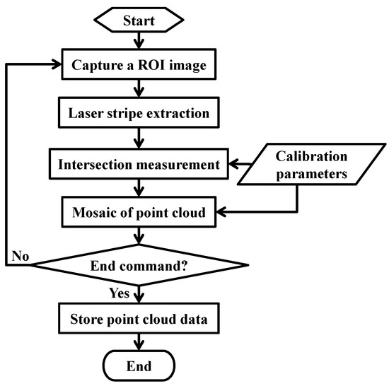
Figure 7. The flowchart of the online measurement procedure.

4.1. Laser Stripe Extraction

Laser stripe extraction is the fundamental step to locate the ROI. The laser line in the images is expected to be single-pixel width ideally. However, there is a line width for the laser employed in practice, which is much wider than the width expected. Thus, the first step of measurement is laser stripe extraction. As the laser stripe conforms to a Gaussian distribution in the vertical direction theoretically, a Gaussian filter is generally employed as the image preprocessing for laser stripe extraction. After the preprocessing, a weighted centroid localization algorithm is carried out to obtain sub-pixel location.

As it is shown in Figure 8, the laser stripe in the image generally possesses the higher grey level. Therefore, it is easy to obtain the binary image of a laser stripe by a threshold method and some other image preprocessing. Furthermore, the minimum bounding box of laser stripe is achieved by a common connected components algorithm. Suppose the bounding box is a $m\times n$ binary matrix $L_{m\times n}$, in which the laser pixels are labeled as 1 while others are 0. Considering the grey level weighting, the weighted matrix of laser $W{L}_{m\times n}$ is expressed as Equation (13).

$$W{L}_{m\times n}=\mathrm{times}\left(L_{m\times n},I_{m\times n}\right).$$

(13)

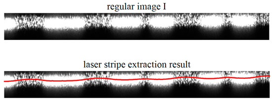
Figure 8. Regular image and laser stripe extraction result (red line).

$I_{m\times n}$ is the corresponding region of the laser bounding box in the regular grey image. $\mathrm{Times}\left(a,b\right)$ represent the element-by-element multiplication of two matrixes $a$ and $b$, which are in the same size. Suppose that the direction of the laser line is along the columns of $W{L}_{m\times n}$ as it is shown in Figure 8, the sub-pixel result of laser stripe extraction $Lo{L}_{m\times 1}$ is located by Equation (14).

$$Lo{L}_{m\times 1}=\mathrm{times}\left(W{L}_{m\times n}·C_{n\times 1},\frac{1}{{\mathrm{sum}}_{col}\left(W{L}_{m\times n}\right)}\right),$$

(14)

where $C_{n\times 1}={\left[1,2,\cdots ,n\right]}^T$ represents a coordinate column vector. ${\mathrm{sum}}_{col}(*)$ is the function to calculate the sum of the matrix in columns. $Lo{L}_{m\times 1}$ is the sub-pixel location of the laser stripe with grey level weighting, which remains a single point in the direction of line width. The result is shown in Figure 8.

4.2. Intersection Measurement

As the calibration results and the laser stripe location are achieved, it is available to calculate the coordinate of points in the camera coordinate system by forward intersection. Generally, the camera coordinate system $X_C{Y}_C{Z}_C$ is regarded as the world coordinate system.

Suppose a point $p\left(u,v\right)$ in laser stripe extraction $Lo{L}_{m\times 1}$, and the corresponding coordinate in the camera coordinate system is $\left(x_c,y_c,z_c\right)$. The equation of the camera optical line is expressed as Equation (5), while the equation of the laser plane is not determined. In the system structure calibration, only the unit normal direction of the laser plane in the camera coordinate system is obtained.

As it is mentioned in single camera calibration, the calibration cannot recover the last component $t_{zi}$ of the translation vector $t$, so $t_{zi}$ can be set to any value, which means the camera coordinate system $X_C{Y}_C{Z}_C$ is able to translate through the $Z_C$ axis. Therefore, when the origin $o_C$ of the camera coordinate system $X_C{Y}_C{Z}_C$ is selected as the intersected point of the $Z_C$ axis and the laser plane, the laser plane equation in the camera coordinate system $X_C{Y}_C{Z}_C$ is determined as Equation (15).

$$n_p^T{\left(x_c,y_c,z_c\right)}^T=0$$

(15)

$n_p={\left(n_{p1},n_{p2},n_{p3}\right)}^T$ is the unit normal direction of laser plane in the camera system. Thus, combining Equations (5) and (15), the intersection measurement result of the laser line point is achieved in a camera coordinate system as follows. By the same method, the 3D coordinates of the located points on the laser line can be generated.

$$P_c={\left[x_c,y_c,z_c\right]}^T={\left[\frac{u-u_0}{m},\frac{v-v_0}{m},-\frac{n_{p1}·\left(u-u_0\right)+n_{p2}·\left(v-v_0\right)}{n_{p3}·m}\right]}^T.$$

(16)

4.3. Mosaic of Measured Points

For every captured image, the point cloud of the laser location is achieved in the camera coordinate. As the displacement platform moved, a series of point clouds is obtained. Though the point cloud obtained from different image is all in the camera coordinate, it is independent actually because the camera is fixed. In order to generate the point cloud for the whole ROI, it is significant to combine the point cloud obtained from each image together, which is the mosaic procedure.

Suppose $d_i$ is the movement distance of the displacement platform when the i-th image is captured. As the unit motor direction of the platform $n_d$ is calibrated, the translation of the platform during the time from the first image captured to the i-th image captured in camera coordinate is $d_i\cdot n_d$. The intersection point in the i-th image is adjusted as Equation (17).

$$P_w=P_{c-i}-d_i\cdot n_d.$$

(17)

$P_{c-i}{\left(x_{c-i},y_{c-i},z_{c-i}\right)}^T$ is the intersection result in the i-th image, while $P_w{\left(x_w,y_w,z_w\right)}^T$ is the final mosaic result of the corresponding point in the camera coordinate system of the first capture.

5. Experiments

In this section, the uncertainty analysis in experiments is presented. The experiments are carried out to demonstrate the performance of the proposed system, and the proposed system is presented in Figure 9. Before the experiments, calibration described in Section 3 is carried out, and the calibration results and the corresponding relative uncertainty are listed in Table 1, in which the uncertainties of $m,n_p,n_d$ are achieved with a statistical method.

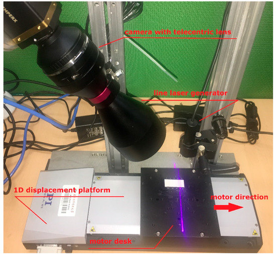
Figure 9. Experimental setup of the proposed telecentric surface reconstruction system.

Table 1. Calibration parameters in experiments.

Parameters	Value	$\mathbf{Uncertainty} \left(1\mathit{\sigma }\right)$
$M$	0.426920	0.000002
$n_p$	(−0.00982, −0.86241, 0.50612)	(0.00002, 0.00035, 0.00059)
$n_d$	(−0.02641, −0.86659, 0.49832)	(0.00005, 0.00005, 0.00009)

It is indicated from the calibration results that $n_p$ and $n_d$ are nearly in parallel, which means the laser plane is nearly perpendicular to the motor desk surface. The practical intersection angle for the system established is $30.4°$ while the intersection angle designed is $30°$. With the calibration parameters, online measurement in Section 4 is realized to acquire the point cloud of ROI.

5.1. Uncertainty Analysis

As the point cloud of ROI is obtained by the measurement procedure mentioned, it is necessary to evaluate the uncertainty of the measured results. Guide on the expression of uncertainty in measurement (GUM) is one of the international standards to evaluate the measurement uncertainty [22]. Since a measurand is usually determined from some other quantities through a functional relationship rather than measured directly, GUM requires the function model which reflects the relationship to achieve the measured uncertainty. The model for the proposed system is expressed in Equation (18), which is determined by combining Equations (16) and (17).

$$P_w=\left[\begin{array}{c}{x}_w\\ y_w\\ z_w\end{array}\right]=\left[\begin{array}{c}\frac{\left(u-u_0\right)}{m}-d\cdot n_{d1}\\ \frac{\left(v-v_0\right)}{m}-d\cdot n_{d2}\\ -\frac{\left[n_{p1}\left(u-u_0\right)+n_{p2}\left(v-v_0\right)\right]}{n_{p3}m}-d\cdot n_{d3}\end{array}\right].$$

(18)

Equation (18) can be rewritten as a function model $P_w=f\left(m,n_p,n_d,p,d\right)$, in which $p\left(u,v\right)$ is the image coordinate of the laser line location. $n_p={\left(n_{p1},n_{p2},n_{p3}\right)}^T$ and $n_d={\left(n_{d1},n_{d2},n_{d3}\right)}^T$ are the unit normal directions of the laser plane and the unit motor direction of the displacement platform in the camera system, respectively. Nevertheless, the measurand required usually is not $P_w$, but $\mathsf{\Delta }{P}_w$, which is the relative position for the measured points. According to Equation (18), the model of $\mathsf{\Delta }{P}_w$ for $P_{w1}=f\left(m,n_p,n_d,p_1,d_1\right)$ and $P_{w2}=f\left(m,n_p,n_d,p_2,d_2\right)$ is presented in Equation (19)

$$\mathsf{\Delta }{P}_w=\left[\begin{array}{c}\mathsf{\Delta }{x}_w\\ \mathsf{\Delta }{y}_w\\ \mathsf{\Delta }{z}_w\end{array}\right]=\left[\begin{array}{c}{x}_{w1}-x_{w2}\\ y_{w1}-y_{w2}\\ z_{w1}-z_{w2}\end{array}\right]=\left[\begin{array}{c}\frac{\left(u_1-u_2\right)}{m}-(d_1-d_2)\cdot n_{d1}\\ \frac{\left(v_1-v_2\right)}{m}-(d_1-d_2)\cdot n_{d2}\\ -\frac{\left[n_{p1}\left(u_1-u_2\right)+n_{p2}\left(v_1-v_2\right)\right]}{n_{p3}m}-(d_1-d_2)\cdot n_{d3}\end{array}\right]$$

(19)

For the function model above $\mathsf{\Delta }{P}_w\triangleq g\left(X\right)$, there are 3 outputs and 13 inputs considering every component of vectors. Thus, the uncertainty of $\mathsf{\Delta }{P}_w$ is defined by the uncertainty propagation formula as Equation (20).

$$V\left(\mathsf{\Delta }{P}_w\right)=J\cdot V\left(X\right)\cdot J^T.$$

(20)

$J$ is the Jacobian matrix of the function model $\mathsf{\Delta }{P}_w=g\left(X\right)$, and $V\left(X\right)$ is the covariance matrix which consists of the uncertainty and covariance of the inputs. The uncertainty of calibration parameters is listed in Table 1. Besides, the uncertainty of $d$ is 0.017, which is decided by the equipment design resolution. The uncertainty of laser line location $\left(u,v\right)$ in the image is $\left(0,0.01\right)$ pixel given the laser stripe extraction algorithm is searching for the location along a single direction of the image. Note that all the inputs are independent except for the components of the unit vector, so the covariance between the components of $n_p$ and $n_d$ should be computed respectively while others are simply set to 0. $V\left(\mathsf{\Delta }{P}_w\right)$ is supposed to be a $3\times 3$ matrix as there are 3 outputs, and the diagonal elements of $V\left(\mathsf{\Delta }{P}_w\right)$ are just the squares of the corresponding output uncertainties.

Once the measure points are settled, the uncertainty of $\mathsf{\Delta }{P}_w$ can be achieved with $V\left(\mathsf{\Delta }{P}_w\right)$. Furthermore, note that the world coordinate system here usually is not the coordinate system desired, the uncertainty of the corresponding Euclidean distance for $\mathsf{\Delta }{P}_w$ is calculated, which is generally more available. For the calibrated system, consider a measured region where Length $\times$ Width $\times$ Height ($L\times W\times H$) is $20\times 40\times 1{ \mathrm{mm}}^3$, in which Width is the direction of the displacement platform, the uncertainty of the Euclidean distance between two points computed with simulation. Without loss of generality, one point is at the corner of the measured region and another point moves from the formal point to another corner along the diagonal of the measured region. The depth varies randomly within 1 $\mathrm{mm}$. The corresponding uncertainty result obtained from the uncertainty propagation formula is shown in Figure 10.

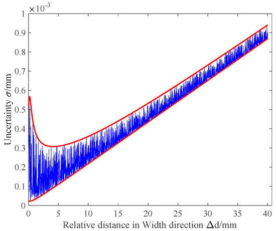
Figure 10. Uncertainty of the calibrated system from simulation. The blue line presents the uncertainty of measurement result, and the red line defines the envelope lines of the uncertainty.

The measured uncertainty fluctuates with the depth random change, meanwhile it rises with the increasing $\mathsf{\Delta }d$, which is the relative distance in the Width direction. The upper and lower bounds of uncertainty for corresponding $\mathsf{\Delta }d$ are labeled with a red line in Figure 10. It is indicated from the result that the uncertainty of measured Euclidean distance $D$ can be simplify as Equation (21).

$$U\left(D\right)=\{\begin{array}{c}0.6\left(\mathsf{\mu }\mathrm{m}\right), \mathsf{\Delta }d\le 20 \mathrm{mm}\\ 0.02\times \mathsf{\Delta }d+0.2, 20<\mathsf{\Delta }d\le 40 \mathrm{mm}\end{array}.$$

(21)

5.2. Results

First of all, a step master is employed to evaluate the performance of the system designed, which is widely used in the evaluation for surface metrology. The step master used in the experiment is 516–499 Cera Step Master 300 C, Mitutoyo, Kanagawa 213-8533, Japan, which has 5 steps designed and the nominal steps are 20, 50, 100, 300 ($\mathsf{\mu }\mathrm{m}$), respectively. The uncertainty of the nominal steps is 0.20 $\mathsf{\mu }\mathrm{m}$ while the variation for each single step is within 0.05 $\mathsf{\mu }\mathrm{m}$. The measured result for the step master is shown in Figure 11 as a depth map. Besides, the measured data for steps are utilized to fit planes with a robust estimation, and the results are listed in Table 2.

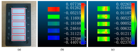
Figure 11. The picture of the step master and the display region (a). Measured depth map of the step master (b) and corresponding off-surface error (c) (unit: mm).

Table 2. Measured result of step master ($\mathsf{\mu }\mathrm{m}$).

Step	1	2	3		4	5
Jump truth		20	50	100	300
Measured value		20.0 ± 0.6	49.5 ± 0.6	100.4 ± 0.6	299.1 ± 0.6
Mean error	4.9	5.0	4.7		4.9	6.2
RMS	6.3	6.5	6.1		6.2	7.5

Some other samples are tested with the proposed telecentric surface metrology system, including two pieces of the circuit board and both sides of a coin. The results are shown in Figure 12, and the ROI is about $20\times 40{ \mathrm{mm}}^2\left(L\times W\right)$ in the circuit board test while the design diameter of the coin is 20.5 $\mathrm{mm}$. From the left to right in every row, the images are practicality pictures, results of the ROI and the partial detail region. The ROI and partial detail region are labeled with a blue and red rectangle in the practicality picture, respectively.

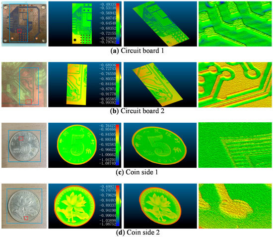
Figure 12. Measured results for some other samples. From left to right, every result presents the practicality picture, measured result in depth map (unit: mm), mesh result of surface reconstruction and partial detail for mesh result of the sample.

6. Discussion

It is indicated from Table 2 that the deviation of the measured value and the designed value is within 1 $\mathsf{\mu }\mathrm{m}$ for each step. However, the error for the step plane is too large to accept. The step master is measured repeatedly, but the result remains stable in the repeatability tests even when the direction of measurement changes. When the effect of random error is excluded, the off-surface error for every point is calculated and the corresponding result is shown in Figure 11. There is an obvious scratch for the plane fit on each step, which is in red and nearly characterized by a linear distribution. The result might be caused by the fact that the step master is used and maintained improperly. From the measured result, it is shown that the obstacle is about 10 to 20 $\mathsf{\mu }\mathrm{m}$ in height; it is a linear inclusion and there is an effect in the vertical direction which obeys an approximately Gaussian distribution. This incident would be a proper instance of the proposed system for a defect-detecting application.

Moreover, several surface reconstruction methods are listed in Table 3 for comparison. The methods listed contain the main measurement approaches based on triangulation, and the lenses employed are telecentric lenses. It is indicated that the accuracy of the active method (structure light and line laser scanning) is better than passive techniques (stereo vision). The employment of binocular telecentric cameras leads to the better performance in structure light. The proposed method performs as well as Hu’s method in accuracy, but the measured region is much larger.

Table 3. Comparison with other methods (unit: mm).

Method	Theory	Equipment	Measured Region	Accuracy
H. Liu [9]	Stereo vision	Two telecentric cameras	40 $\times$ 30	0.009
L. Rao [12]	Structure light	Telecentric camera, telecentric projector	23.7 $\times$ 17.7	0.005
Y. Hu [13]	Structure light	Two telecentric cameras, telecentric projector	10 $\times$ 7	0.0014
Ours	Line laser scanning	Telecentric camera, line laser generator, 1D displacement platform	40 $\times$ 20	0.0009

When we come back to the three main challenges mentioned in introduction, the first challenge, the occlusion due to the principle of triangulation, cannot be completely solved with a single camera while the other two challenges are solved with the proposed methods for system calibration, telecentric intersection and laser stripe extraction. In the proposed system, the unsolved problem is made to be acceptable for the demand with the system design, but it still exists (Figure 13). There is a narrow gap at the position where the depth changes significantly in surface reconstruction, and the width of the gap mainly depends on the intersection angle designed and the jump change of the depth.

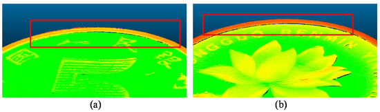
Figure 13. The manifestation of the unmeasured region due to the occlusion in a practical experiment. The unmeasured region is marked with red rectangular for the results of (a) Coin side 1 and (b) Coin side 2.

The speed of the motor stage is set to 0.2 mm/s, so it would take 100 s to measure the region of 20 mm Length. The frame frequency of camera is 40 fps, which means the interval width between the point clouds is 0.005 mm. The measurement speed can be adjusted with the variation of the motor speed. Actually, the measurement speed only affects the density of the point cloud in the plane of $L\times W$. The accuracy in depth remains stable as long as it is captured. Moreover, the speed can be improved with a better camera and displacement platform, and the application of the displacement platform for the proposed method can expand the measurement region continuously.

According to the experimental results, the system designed holds the deviation of less than 1.0 $\mathsf{\mu }\mathrm{m}$ for the region of $20\times 40\times 1{ \mathrm{mm}}^3\left(L\times W\times H\right)$ meanwhile the uncertainty is less than 1.0 $\mathsf{\mu }\mathrm{m}$ in 68% level of confidence. The measurement region is limited by the travel range of the 1D displacement platform under the line laser (20 mm) and the size of the telecentric lens (40 mm). The $1 \mathrm{mm}$ presented indicates the practical variation interval for the measured object, which is utilized in the uncertainty calculation. The measurement ability of depth depends on the depth of field of the telecentric lens employed, which is 6.8 mm. The test on the step master indicates that it is available for the proposed system to be applied in surface detection applications, such as defect detection and circuit board tests.

7. Conclusions

A telecentric surface metrology system based on laser scanning is proposed to realize micro-scale surface detecting in a way of non-contact measurement. The system consists of a single camera with a telecentric lens, line laser generator and 1D displacement platform. The system parameters designed are analyzed and a practical system for the concrete application is established. Based on the system designed, flexible calibration methods are employed to achieve high-accuracy calibration for the system parameters, including camera parameters and system structure parameters. With the calibration parameters, the system measures the ROI in the procedure of laser stripe extraction, intersection measurement, and mosaic of the point cloud in turn. The uncertainty of measurement is derived in terms of the measured function model with uncertainty propagation formula. Step master and other samples are measured to indicate the performance of the system designed. Experimental results illustrate that the proposed system has prominent advantages in accuracy compared with previous methods.

References

- Shirmohammadi, S.; Ferrero, A. Camera as the instrument: The rising trend of vision based measurement. IEEE Instru. Meas. Mag. 2014, 17, 41–47. [Google Scholar] [CrossRef]
- Espino, J.G.; Gonzalez-Barbosa, J.J.; Loenzo, R.A.; Esparza, D.M.; Gonzalez-Barbosa, R. Vision System for 3D Reconstruction with Telecentric Lens. In Mexican Conference on Pattern Recognition; Springer: Berlin/Heidelberg, Germany, 2012. [Google Scholar]
- Zhang, J.; Chen, X.; Xi, J.; Wu, Z. Aberration correction of double-sided telecentric zoom lenses using lens modules. Appl. Opt. 2014, 53, 6123. [Google Scholar] [CrossRef]
- Mikš, A.; Novák, J. Design of a double-sided telecentric zoom lens. Appl. Opt. 2012, 51, 5928. [Google Scholar] [CrossRef] [PubMed]
- Kim, J.S.; Kanade, T. Multiaperture telecentric lens for 3D reconstruction. Opt. Lett. 2011, 36, 1050–1052. [Google Scholar] [CrossRef]
- Xu, J.; Gao, B.; Liu, C.; Wang, P.; Gao, S. An omnidirectional 3D sensor with line laser scanning. Opt. Lasers Eng. 2016, 84, 96–104. [Google Scholar] [CrossRef]
- Li, B.; Zhang, S. Microscopic structured light 3D profilometry: Binary defocusing technique vs. sinusoidal fringe projection. Opt. Lasers Eng. 2017, 96, 117–123. [Google Scholar] [CrossRef]
- Chen, Z.; Liao, H.; Zhang, X. Telecentric stereo micro-vision system: Calibration method and experiments. Opt. Laser Eng. 2014, 57, 82–92. [Google Scholar] [CrossRef]
- Liu, H.; Zhu, Z.; Yao, L.; Dong, J.; Chen, S.; Zhang, X.; Shang, Y. Epipolar rectification method for a stereovision system with telecentric cameras. Opt. Lasers Eng. 2016, 83, 99–105. [Google Scholar] [CrossRef]
- Beermann, R.; Quentin, L.; Kästner, M.; Reithmeier, E. Calibration routine for a telecentric stereo vision system considering affine mirror ambiguity. Opt. Eng. 2020, 59, 054104. [Google Scholar] [CrossRef]
- Aloimonos, J.; Weiss, I.; Bandyopadhyay, A. Active vision. Int. J. Comput. Vis. 1988, 1, 333–356. [Google Scholar] [CrossRef]
- Rao, L.; Da, F.; Kong, W.; Huang, H. Flexible calibration method for telecentric fringe projection profilometry systems. Opt. Express 2016, 24, 1222–1237. [Google Scholar] [CrossRef]
- Hu, Y.; Chen, Q.; Feng, S.; Tao, T.; Asundi, A.; Zuo, C. A new microscopic telecentric stereo vision system—Calibration, rectification, and three-dimensional reconstruction. Opt. Lasers Eng. 2019, 113, 14–22. [Google Scholar] [CrossRef]
- Zhang, S.; Li, B.; Ren, F.; Dong, R. High-Precision Measurement of Binocular Telecentric Vision System with Novel Calibration and Matching Methods. IEEE Access 2019, 7, 54682–54692. [Google Scholar] [CrossRef]
- Xi, F.; Shu, C. CAD-based path planning for 3-D line laser scanning. Comput. Aided Des. 1999, 31, 473–479. [Google Scholar] [CrossRef]
- Usamentiaga, R.; Molleda, J.; García, D.F. Fast and robust laser stripe extraction for 3D reconstruction in industrial environments. Mach. Vision Appl. 2012, 23, 179–196. [Google Scholar] [CrossRef]
- Dang, Q.K.; Chee, Y.; Pham, D.D.; Suh, Y.S. A virtual blind cane using a line laser-based vision system and an inertial measurement unit. Sens. Basel 2016, 16, 95. [Google Scholar] [CrossRef] [PubMed]
- Isa, M.A.; Lazoglu, I. Design and analysis of a 3D laser scanner. Measurement 2017, 111, 122–133. [Google Scholar] [CrossRef]
- Son, S.; Park, H.; Lee, K.H. Automated laser scanning system for reverse engineering and inspection. Int. J. Mach. Tool Manuf. 2002, 42, 889–897. [Google Scholar] [CrossRef]
- Yao, L.; Liu, H. A Flexible Calibration Approach for Cameras with Double-Sided Telecentric Lenses. Int. J. Adv. Robot. Syst. 2016, 13, 82. [Google Scholar] [CrossRef]
- Guan, B.; Yao, L.; Liu, H.; Shang, Y. An accurate calibration method for non-overlapping cameras with double-sided telecentric lenses. Optik 2017, 131, 724–732. [Google Scholar] [CrossRef]
- JCGM. Evaluation of Measurement Data—Guide to the Expression of Uncertainty in Measurement (GUM 2008); BIPM: Paris, France, 2008. [Google Scholar]
Publisher’s Note: MDPI stays neutral with regard to jurisdictional claims in published maps and institutional affiliations. |
© 2021 by the authors. Licensee MDPI, Basel, Switzerland. This article is an open access article distributed under the terms and conditions of the Creative Commons Attribution (CC BY) license (http://creativecommons.org/licenses/by/4.0/).