Abstract
Using recycled aggregate in concrete is one of the best ways to reduce construction pollution and prevent the exploitation of natural resources to provide the needed aggregate. However, recycled aggregates affect the mechanical properties of concrete, but the existing information on the subject is less than what the industry needs. Compressive strength, on the other hand, is the most important mechanical property of concrete. Therefore, having predictive models to provide the required information can be helpful to convince the industry to increase the use of recycled aggregate in concrete. In this research, three different optimization algorithms including genetic algorithm (GA), salp swarm algorithm (SSA), and grasshopper optimization algorithm (GOA) are employed to be hybridized with artificial neural network (ANN) separately to predict the compressive strength of concrete containing recycled aggregate, and a M5P tree model is used to test the efficiency of the ANNs. The results of this study show the superior efficiency of the modified ANN with SSA when compared to other models. However, the statistical indicators of the hybrid ANNs with SSA, GA, and GOA are so close to each other.
1. Introduction
Every year, a massive proportion of construction and demolished waste (C&DW) is produced all around the world. For instance, the USA produces around 250 million tons [1], China produces almost two billion tons [2], and the European Union is responsible for about 900 million tons of C&DW [3]. Using C&DWs as recycled aggregate has two benefits. First, it reduces the amount of C&DW that needs to be disposed. Second, it reduces the demand for regular aggregate.
Recycled aggregate as an environmental alternative in concrete projects is a promising environmental solution to reduce the carbon footprint of construction projects. Sourced from C&DW, it comes with varying properties depending on the type of the structure being demolished/built. As in some buildings, the dominant material used might be timber, concrete, or steel which ultimately changes the portion of recycled aggregate. The properties of aggregates vary a lot depending on their source and the manufacturing process. The influence of these two factors, i.e., the source and the process, is mainly on the porosity, water absorption, and saturated surface dried ratio, all of which significantly affect the final performance of concrete, made with these aggregates [3]. In most of the cases, a poor mechanical performance results after using recycled aggregate in concrete and that is the major reason behind the lack of tendency from the consumer’s perspective in using more of this environmental alternative [4,5,6,7].
As the amount of recycled aggregate that used in concrete increases, the elastic modulus, compressive strength and density of the concrete decrease [8,9,10,11]. However, the use of recycled aggregate is allowed in specific amounts in some standards [8]. On the other hand, in case of service life and durability, there are some studies that showed these properties of concrete with recycled aggregate are not as good as those of conventional concrete [12,13] while others concluded that concrete with recycled aggregate has better durability than conventional concrete [14]. While there is no commercial approach for the use of high-quality recycled aggregate, the consumers can still be motivated to use more of recycled aggregate upon the availability of more data.
Artificial intelligence and data mining techniques have proven to be solutions to provide the end users with a reliable information in regards to the mechanical properties of concrete. Recently, predictive models based on artificial intelligence methods have been used to forecast the mechanical properties of concrete and predict the effect of changes in its mixture design on its behavior [15,16,17,18,19,20,21,22,23,24,25,26,27,28,29,30,31,32,33,34,35,36,37,38,39,40,41,42,43,44,45,46,47,48,49,50,51,52,53,54,55,56,57]. For instance, Behnood and Golafshani [37], has used M5P three model to estimate mechanical properties of concrete containing used foundry sand. Their results show that the M5P three model has an acceptable performance to predict the properties of concrete. Zhang et al. [23] have developed a model by hybridizing beetle antennae search (BAS) and multi-output least square support vector regression (MOLSSVR) to predict concrete’s compressive strength (CS) and permeability coefficient of pervious. The outcomes of this research indicated that their proposed model performs better than support vector regression (SVR), MOLSSVR, logistic regression, and modified ANN with firefly algorithm. In another research, Ashrafian et al. [54] used chi-square automatic interaction detection, M5P tree model, M5rule, and random forest to forecast mechanical properties of roller-compacted concrete pavement. It was observed that the predicted values of random forest had lower errors and higher correlation in comparison with other models. Kandiri et al. [40] developed a hybrid ANN with multi-objective salp swarm algorithm to estimate CS of concrete with ground granulated blast furnace slag. In that research, it was showed that 13 out of 19 ANNs outperformed M5P tree model. In another Article, by hybridizing ANFIS and ANN with grey wolf optimizer, Golafshani et al. [49] showed that an ANN-based model was more efficient than a modified ANFIS. Recently, probabilistic approaches have been used to obtain the uncertainties that influence concrete characteristics [58,59,60,61]. For instance, Ramezani et al. [58] used the Kelly-Tyson theory to propose a probabilistic model for predicting the flexural strength of carbon nanotubes–cement nanocomposites. The results showed that the proposed model is able to obtain the experimental observation with an acceptable performance.
However, ANN’s performance is directly affected by its architecture. The number of its hidden layers and neurons in them is constant for each ANN. In fact, once the network is set, these parameters are unchangeable. Usually, these parameters are obtained by trial-and-error method, in which a lot of time is spent on reaching the optimum architecture, and sometimes obtaining the optimum architecture is impossible. Therefore, an algorithm that can optimize an ANN architecture is needed. In this study, ANN’s architecture is optimized with three optimization algorithms including grasshopper optimization, salp swarm algorithm, and genetic algorithm. Then, the results of these models are compared with M5P tree model, which is a classification-based regression model. To develop the models, data had been collected from 12 different scientific resources all with mutual mixing and experimental methods to avoid inconsistency of the output analysis [62,63,64,65,66,67,68,69,70,71]. The next section explains the data gathering procedure followed by a section of describing optimization methods, ANN, the modified proposed models, and M5P three model. After that, the results are analyzed and compared with each other.
2. Data Gathering
For developing a predictive model, there is a need for a valid dataset. The dataset needs to include all the parameters, which are possible to be effective on the outputs as inputs, except those that are constant among all records. In the present research, a dataset including 234 patterns was collected from literature [62,63,64,65,66,67,68,70,71,72,73,74,75]. In all patterns, the curing condition were the same, and the used cement was ordinary Portland cement (OPC). Moreover, the superplasticizer (SP) in all mixes was Polycarboxylican, and the type of specimen in all recorded patterns were cube with the same size (100 mm by 100 mm). The inputs of the models in this study are the testing age (TA), the amount of OPC, sand (S), coarse aggregate (CA), fine aggregate (FA), the ratio of water to cement (W/C), superplasticizer to cement by percentage (SP/C), the ratio of recycled coarse aggregate to total coarse aggregate (CRA), and the ratio of recycled fine aggregate to total fine aggregate (FRA). The only output variable of the models is the CS. Figure 1 shows the histogram of the inputs and output variables. Furthermore, the anatomical statistics of the gathered dataset are represented in Table 1.
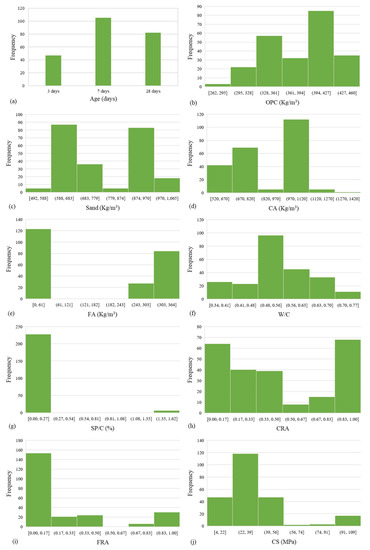
Figure 1.
Output and input variables’ histogram: (a) ages of samples, (b) the amount of OPC, (c) the amount of sand, (d) the amount of coarse aggregate, (e) the amount of fine aggregate, (f) the ratio of water to cement, (g) the ratio of superplasticizer to cement by percentage, (h) the ratio of recycled coarse aggregate to total coarse aggregate, (i) the ratio of recycled fine aggregate to total fine aggregate, and (j) compressive strength.

Table 1.
Anatomical statistics of the inputs and output.
3. Optimization Algorithms
Big optimization problems with many parameters cannot be solved by accurate mathematically methods. Therefore, heuristic and metaheuristic algorithms are served to find the best answer possible in a convenient time. Metaheuristic algorithms that are developed inspired by nature are the most popular ones [30,40]. Most of these algorithms include exploration and exploitation. In the exploration phase the possible solutions that are far from each other are studied. In the exploitation phase, the possible solutions that are close are checked. In fact, exploration phase helps the algorithm to avoid local optimums.
3.1. Genetic Algorithm (GA)
The genetic algorithm is a metaheuristic algorithm for solving optimization problems which was proposed by John Holland [76]. In this algorithm, data are recorded in chromosomes, and each individual’s chromosomes is allocated to a pattern. Every two individuals make two offspring by crossover and mutation methods. GA includes mutation and crossover that are responsible for exploration and exploitation phases, respectively. A number of individuals equal to the number of the initial population are going to survive based on their fitness functions. In other words, the fitness value of each individual (parents and offspring) are calculated and those who have better fitness value have better chances to live. In this study, the survivors are selected by roulette wheel. In this method, the chance of surviving chance is defined as follow:
where, is the fitness function for the kth individual, is the probability of choosing kth individual, n is the population size, and it is obvious that . Algorithm 1 represents different steps of a GA algorithm. This algorithm has been used to train an ANN in a number of previous studies [17,32,44,47,57,77].
| Algorithm 1: Pseudocode of genetic algorithm. |
| 1: Generate initial population |
| 2: i = 1 |
| 3: while (i < number of iterations) |
| 4: Calculate the fitness function of the each individual |
| 5: Select parents |
| 6: Recombine pairs of parents |
| 7: Create offspring from parents via crossover |
| 8: Apply mutation to offspring |
| 9: end while |
| 10: Return the individuals that obtain the best fitness |
3.2. Salp Swarm Algorithm (SSA)
Salps belong to Salpidae group, which are look like jellyfishes, with a body shape like transparent barrel [78]. Usually, they tend to create a chain to have fast coordination for finding food. SSA is inspired by their swarm intelligence. The salp chain has a leader, which is the salp at the front, and followers, which are the rest of the group. The leader is responsible for exploration and the followers handle the exploitation phase. Each salp has a position, which is defined in a search space with n dimensions, where n is the decision variables’ number in the optimization problem. The following equation updates the leader position.
where is rth dimension of the leader position, is the position of the food, and are the upper and the lower bounds in the rth dimension, respectively. In addition, balances exploration and exploitation phases; and are random numbers in [0,1]. is calculated as follows:
where is the maximum number of iterations and represents the current iteration. The position of the followers are calculated as follows:
where is position of the ith salp in the rth dimension. Now, it is possible to simulate the salp swarm. Algorithm 2 illustrates pseudo cod of SSA. This algorithm has been used to train an ANN in a number of previous studies [35,40,43,79].
| Algorithm 2: Pseudocode of SSA. |
| 1: Initiate salp population considering the upper and lower bounds |
| 2: i = 1 |
| 3: while (i ≤ number of iterations) |
| 4: Calculate fitness function for each salp |
| 5: Choose the best salp as the food source |
| 6: Determine the value of d1 using Equation (3) |
| 7: for each salp |
| 8: if (i = 1) |
| 9: Update the position of the leading salp by Equation (2) |
| 10: else |
| 11: Update the position of the follower salp by Equation (4) |
| 12: end |
| 13: end |
| 14: Correct the positions of the salps considering upper and lower bounds |
| 15: end |
| 16: Return the food source |
3.3. Grasshopper Optimization Algorithm (GOA)
Grasshoppers are kinds of insects that are observed individually in nature. They live in a huge swarm in both nymph and adulthood phases [80,81]. In contrast to their nymph phase in which their swarm takes move in small steps, in adulthood phase they take long-range steps. The GOA algorithm is defined based on their behavior where the small steps are considered for exploitation phase and big steps are used for exploration phase. Like SSA, every grasshopper search agent has a position () made of n-dimension, which is defined as follows:
where , , and are, respectively, social interaction, gravity force, and wind advection on the jth search agent, and , , and are random number between zero and one to make random behavior. The following equation discuss the social interaction ():
where drm is the distance between the rth and mth grasshopper, computed as , is a unit vector from the rth to mth grasshopper, computed as , and s is a function to describe the social forces’ strength represented as follows:
where and are the intensity of attractive and attraction length scale, respectively. Based on the distance between two grasshoppers, they apply force on each other. This force could be absorption for far grasshoppers and repulsion for close grasshoppers. However, there is an exact value of distance, in which grasshoppers apply no force on each other, which called comfort zone. Moreover, and are calculated as follows:
where and are the constant of gravity and a unity vector towards the earth’s center, respectively, and and are the constant of gravity drift and a unity vector in the wind‘s direction, respectively. A modified version of the Equation (5) is represented as follows:
where and are the upper bound and the lower bound in the qth dimension, respectively, is the qth dimension of the target position, h is a decreasing coefficient to shrink the comfort zone. In the first iteration the rate of exploration is higher than that in the final iterations. Therefore, h should decrease as the algorithm get close to its end. The h parameter is calculated as follows:
where IT is the number of maximum iterations and hmax and hmin are 1 and 0.00001, respectively. Algorithm 3 represents the different steps of the GOA.
| Algorithm 3: Pseudocode of GOA. |
| 1: Initiate random grasshopper population considering the upper and lower bounds |
| 2: Calculate the fitness function for each grasshopper |
| 3: Target = best grasshoppers |
| 4: B = Maximum number of iterations |
| 5: b = 1 |
| 6: while (b < B) |
| 7: Update h using Equation (11) |
| 8: N = the number of grasshoppers |
| 9: for each grasshopper |
| 10: Normalize the distance between grasshoppers in [1,4] |
| 11: Update the position of the current grasshopper using Equation (10) |
| 12: Correct the grasshopper position considering boundaries |
| 13: end |
| 14: Update Target |
| 15: b = b + 1 |
| 16: end |
| 17: Return Target |
3.4. Artificial Neural Network (ANN)
ANN is an AI based method that simulates human brain to learn machines. ANN can solve new problems using past experiences like human brain. The most popular type of ANN is multi-layer perceptron (MLP). An MLP has an input layer (IL), which receives inputs from the patterns, a number of hidden layers (HL), which is responsible for processing, and an output layer (OL) that returns the output. IL and OL include a number of neurons equal to inputs and outputs, respectively. Figure 2 illustrates a schematic MLP.
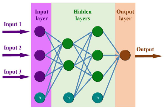
Figure 2.
A schematic MLP.
Every node is linked to the nodes in the next layer with linking weights. The IL’ nodes just receive the inputs and give them to the next layer. HLs’ neurons take the outputs of the past layer’s neurons, sum them, and put them in the activation function. The OL’s nodes take their inputs from the previous layers’ nodes, sum them, and return the answer as the network’s outputs. There are various activation functions for ANNs such as sigmoid, tangent sigmoid, linear, and hyperbolic tangent sigmoid to name a few. In fact, the main problem of an ANN is to obtain the best weights for links where there are a number of algorithms for solving this problem. The most used problem-solving algorithm for ANNs is feed-forward back-propagation (FFBP) [82,83]. In FFBP algorithm, weights are predicted from the IL to OL, but improved from the OL to IL by learning algorithms. Among learning algorithms, Levenberg-Marquardt (LM), due to its better speed and performance, is the best one to predict concrete behavior [40,84]. In the LM algorithm, the updated weights and bias are calculated as follows:
where wbt+1 and J are the updated weights and biases and the Jacobian matrix that includes the first derivatives of the network errors concerning the weights and biases. µ, I, and e are a positive real number damping factor, identity matrix, and vector of ANNs error, respectively. A schematic neuron is shown is Figure 3.
wbt+1 = wbt − [JTJ + μ I]−1 JT e
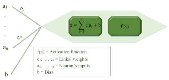
Figure 3.
A schematic neuron.
The performance of an ANN is affected by its structure, and trial-and-error is the most commonly used method for obtaining the best structure. Using this method can cost a huge amount of time and energy, although there is a possibility of not gaining the best architecture. Hence, having a systematic method to reach the ANN’s best architecture is necessary. In the present study, an ANN is modified using GA, SSA, and GOA, separately. The gene of an individual and the position of a salp and grasshopper are divided into two parts. The first part is allocated to the number of HL. According to the Figure 4, the ith value of the first part can be zero or one. If it is zero, the ith HL is deactivated, and it is activated if the ith value of the first part is one. The second part, on the other hand, is related to the number of neurons in each HL. For instance, if the jth value of the second part is 11, it means there is 11 neurons in the jth HL.
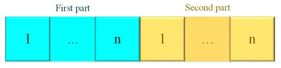
Figure 4.
Position of a salp and a grasshopper and chromosome of an individual.
The process of each model is almost the same as its optimization algorithm, except that their fitness are calculated by ANN’s error, and ANN uses RMSE to compute the error.
where Q is number of records, is the Measured results and is predicted values related to the qth record.
3.5. M5P Tree
The M5P tree is the improved version of M5 tree that consist of three phases: dividing the input space, building the tree and deriving the knowledge [85]. The M5P tree, on the other hand, includes four Phases. The first phase includes building a full tree by splitting the data using the selected parameters and a division criterion. By using standard deviation reduction parameter (SDRP), the search space is split. SDRP is represented as follows:
where || is the set’s number elements, dr is rth sub-space gained by splitting the node according to selected divided parameter, sd is the standard deviation, and D is the dataset which reaches the node. This process is applied recursively until the patterns at a node either contains only a small number of sets or having negligible variations. The following phase includes developing a linear regression at each node. In the next phase, a pruning process is executed to catalyze the computing efficiency and avoid over-fitting. In the last phase, to deal with the sharp discontinuities that are results of data branching, the smoothing process is executed. The smoothing parameter is represented as follows:
where is the calculated value passed up to the next higher node; a, b, r, and s are, respectively, the calculated target at this node, the model’s estimated output at the current node, the cardinal number of training set that reach the node, and a smoothing parameter.
4. Results
Before running the models, the data need to be prepared. In the first step, because of having different inputs with different scales, the dataset should be normalized in [−1,1] using following equation:
where is an input value, , , and are normal, maximum and minimum values of the i, respectively. Furthermore, every ANN requires a dataset to train the network, another data set to validate the training process, and a whole other data set to test the network. Usually the datasets are allocated to these phases by randomizing the patterns. The drawback of this method is overfitting. As a result, in the present research, k-fold cross-validation method is employed in which the data records are randomized and split into k fold [26,28,40,82,86,87,88]. Then, the model is run k times, and it uses a fold in each time for validating and testing. For instance, in the ith run, the ith fold is served as validation and testing dataset, and other folds are served for training. When the runs are finished, the average error of k times running the network is represented as the error of the network. Using this method results in that all records are served as training, validating, and testing.
Every model has its own adjustment parameters that need to be determined. The trial-and-error method is the most popular method for this purpose. Therefore, it is employed in the present research. The adjustment parameters of GA, SSA, and GOA are represented in Table 2.
Table 2.
Adjustment parameters of modified ANNs.
After running all models, three ANNs with different architecture, which are optimized by three different algorithms, are made that are illustrated in Figure 5. Moreover, M5P tree model is visualized in Figure 6. According to the Figure 5, hybridized ANN with GA (ANNGA) has a couple of the HLs and eleven neurons in each of them. Moreover, the hybridized ANN with SSA (ANNSSA) contains two HLs with seven neurons in the HL number one and nine neurons in the HL number two, and the hybridized ANN with GOA (ANNGOA) has six neurons in its only HL. Hence, the ANNGOA has the simplest structure while the ANNGA has the biggest structure, and the ANNSSA is in between them. Biases and weights of the ANNs and the coefficient of the M5P tree is represented in the Appendix A.
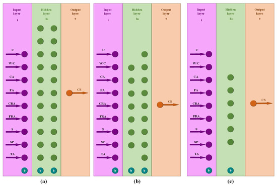
Figure 5.
Architecture of (a) hybridized ANN with GA (ANNGA), (b) hybridized ANN with SSA (ANNSSA), and (c) hybridized ANN with GOA (ANNGOA).
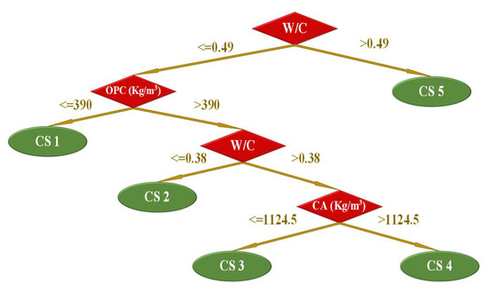
Figure 6.
M5P tree model.
In the present study to have a good comparison among the four models, in addition to RMSE, Pearson correlation coefficient (R), mean absolute percentage error (MAPE), mean absolute error (MAE), mean absolute bias error (MBE), scatter index (SI), and relative square error (RSE) are employed, which are formulated as follow:
where is mean value of measured results, and other parameters are explained in the previous section. MBE indicates that the model overestimates (MBE > 0) or underestimates (MBE < 0). SI determines that the performance of the model is “excellent” (0 ≤ SI < 0.1), “good” (0.1 ≤ SI < 0.2), “fair” (0.2 ≤ SI < 0.3), or “poor” (0.3 ≤ SI). Table 3 represents these indicators.
Table 3.
Statistic indicator of models.
According to Table 3, RMSE of ANNSSA is the lowest with the value of 2.734 MPa, while the M5P has the highest RMSE, which is over 2.5 times bigger than that of ANNSSA. The AANNGA and ANNGOA have the second and third least RMSE, respectively. In the case of MAE, the ANNSSA M5P tree has the highest cost by the value of 5.502 MPa followed by the ANNGOA of which MAE is lower than that of the M5P tree by almost 60%, the same value of ANNGA and ANNSSA are less than that of the M5P tree by 62% and 66%, respectively. According to RSE, the ANNSSA is the most accurate model with the RSE value of 0.017 while the M5P tree model is the least accurate one with the RSE value of 0.149, and ANNGA and ANNGOA are in between. The ANNSSA and ANNGA have almost the same MAPE while this value of the ANNGOA and the M5p tree are more than that of the ANNSSA by 25% and 245%, respectively. MBE indicates that the ANNSSA, the ANNGOA, and the M5P tree overestimate the compressive strength while the ANNGA underestimates that. According to SI, the M5P tree performs well, and other models performances are excellent. The R-values of all models are 0.99, which show a great correlation between measured and predicted compressive strength, except the R-value of M5P tree, which is 0.94. Figure 7 illustrates the predicted vs measured compressive strength, in which it can be seen that the scatter around the base line (linear regression) in ANNSSA is more than others. Moreover, Figure 8 compares MAE, RMSE, and MAPE in order to sort the models based on their efficiency. According to this figure, the ANNSSA is the most efficient model followed closely by the ANNGA and the ANNGOA respectively. Furthermore, the M5P tree is the least efficient model and has the highest error values. This order is true for MAE, RMSE, and MAPE.
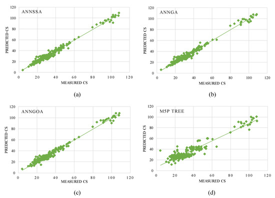
Figure 7.
Predicted vs measured compressive strength for (a) ANNSSA, (b) ANNGA, (c) ANNGOA, and (d) M5P three.
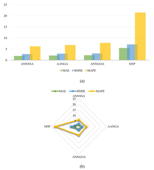
Figure 8.
(a) A bar chart and (b) a radar chart to compare models’ results overlay.
5. Conclusions
A simple ANN saves time and energy, which are spent on obtaining CS of concrete containing recycled aggregate. However, the ANN should be accurate as well to be useful. Otherwise, it just adds to higher costs. In this study, three different optimization algorithms (GA, SSA, and GOA) are employed to modify ANN for that purpose, and M5P tree served as a good comparison model. Results show that all ANNs have better performances than the M5P tree model. Moreover, the ANN that is hybridized with SSA has the lowest values of error, and the second simplest architecture. ANNGOA, on the other hand, has the simplest structure, with the highest values of error, and finally, ANNGA despite of its architecture, which is the most complex one, is the second most accurate model among the ANNs. Although all the ANNs are so close in both accuracy and complexity, the ANNSSA is recommended if accuracy is needed and the ANNGOA should be used if there is a need for simplicity.
The compressive strength (CS) of concrete containing different amounts of recycled aggregate (RA) is shown in Figure 9. According to this figure, increasing the amount of RA to 50% causes a decrease in the CS value at all ages. However, the CS value of the samples with 100% RA is higher than that of the samples with 50% RA at the age of 7 and 28 days, while the CS values of these two classes are almost equal at the age of 3 days.
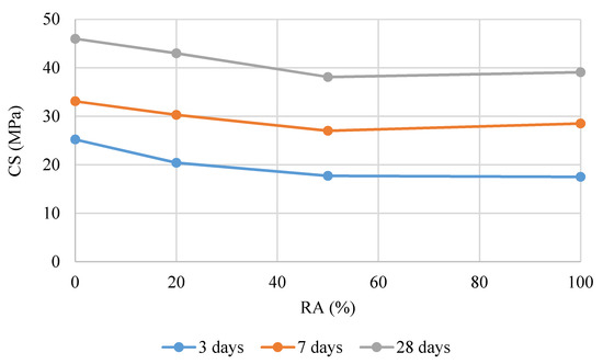
Figure 9.
The CS of concrete with different amounts of RA.
Author Contributions
Conceptualization, A.K. and M.K.; methodology, A.K.; software, A.K.; validation, A.K. and M.K.; formal analysis, A.K.; investigation, A.K.; data curation, F.S.; writing—original draft preparation, A.K. and F.S.; writing—review and editing, A.K. and M.K.; supervision, M.K. All authors have read and agreed to the published version of the manuscript.
Funding
This research received no external funding.
Institutional Review Board Statement
Not applicable.
Informed Consent Statement
Not applicable.
Data Availability Statement
The data presented in this study are available on request from the corresponding author.
Conflicts of Interest
The authors declare no conflict of interest.
Appendix A
Appendix A.1. Biases and Weights of the ANNGOA Model
Appendix A.2. Biases and Weights of the ANNSSA Model
Appendix A.3. Biases and Weights of the ANNGA Model
Appendix A.4. Calculated Coefficient of the MP5 Tree Model
Table A1.
Calculated coefficient for the M5P tree.
Table A1.
Calculated coefficient for the M5P tree.
| Linear Models | Coefficients | |||||||||
|---|---|---|---|---|---|---|---|---|---|---|
| OPC | W/C | CA | FA | CRA | FRA | Sand | SP | TA | Bias | |
| CS1 | −0.3456 | −227.63 | 0.0548 | 0.0277 | 12.8748 | 1.5747 | 0.0148 | 0 | 0.466 | 226.3128 |
| CS2 | −0.1483 | −130.427 | −0.0374 | 0.0277 | −2.681 | 1.5747 | 0.0148 | 0 | 0.4618 | 180.8033 |
| CS3 | −0.2059 | −130.427 | −0.0393 | 0.0277 | −3.4258 | 1.5747 | 0.0148 | 0 | 0.5897 | 204.2375 |
| CS4 | −0.2193 | −130.427 | −0.0489 | 0.0277 | −3.1624 | 1.5747 | 0.0148 | 0 | 0.5241 | 220.4764 |
| CS5 | −0.0233 | 7.2736 | 0.0539 | 0.0764 | −5.6897 | 7.9546 | 0.0363 | 0 | 0.659 | 60.8239 |
References
- Lotfy, A.; Al-Fayez, M. Performance evaluation of structural concrete using controlled quality coarse and fine recycled concrete aggregate. Cem. Concr. Compos. 2015, 61, 36–43. [Google Scholar] [CrossRef]
- Wang, J.; Wu, H.; Tam, V.W.Y.; Zuo, J. Considering life-cycle environmental impacts and society’s willingness for optimizing construction and demolition waste management fee: An empirical study of China. J. Clean. Prod. 2019, 206, 1004–1014. [Google Scholar] [CrossRef]
- Hammoudi, A.; Moussaceb, K.; Belebchouche, C.; Dahmoune, F. Comparison of artificial neural network (ANN) and response surface methodology (RSM) prediction in compressive strength of recycled concrete aggregates. Constr. Build. Mater. 2019, 209, 425–436. [Google Scholar] [CrossRef]
- Figueroa, J.D.; Fout, T.; Plasynski, S.; McIlvried, H.; Srivastava, R.D. Advances in CO2 capture technology-The U.S. Department of Energy’s Carbon Sequestration Program. Int. J. Greenh. Gas Control. 2008, 2, 9–20. [Google Scholar] [CrossRef]
- Rochelle, G.T. Amine Scrubbing for CO2 Capture. Science 2009, 325, 1652–1654. [Google Scholar] [CrossRef] [PubMed]
- Wang, Y.; Zhao, L.; Otto, A.; Robinius, M.; Stolten, D. A Review of Post-combustion CO2 Capture Technologies from Coal-fired Power Plants. Energy Procedia 2017, 114, 650–665. [Google Scholar] [CrossRef]
- Todhunter, A.; Crowley, M.; Sartipi, F.; Jegendran, K. Use of the by-products of post-combustion carbon capture in concrete production: Australian case study. J. Constr. Mater. 2019, 1, 1–22. [Google Scholar] [CrossRef]
- Velay-Lizancos, M.; Martinez-Lage, I.; Azenha, M.; Granja, J.; Vazquez-Burgo, P. Concrete with fine and coarse recycled aggregates: E-modulus evolution, compressive strength and non-destructive testing at early ages. Constr. Build. Mater. 2018, 193, 323–331. [Google Scholar] [CrossRef]
- Medina, C.; Zhu, W.; Howind, T.; Sánchez De Rojas, M.I.; Frías, M. Influence of mixed recycled aggregate on the physi-cal-mechanical properties of recycled concrete. J. Clean. Prod. 2014, 68, 216–225. [Google Scholar] [CrossRef]
- Behnood, A.; Olek, J.; Glinicki, M.A. Predicting modulus elasticity of recycled aggregate concrete using M5′ model tree algorithm. Constr. Build. Mater. 2015, 94, 137–147. [Google Scholar] [CrossRef]
- Etxeberria, M.; Marí, A.R.; Vázquez, E. Recycled aggregate concrete as structural material. Mater. Struct. 2006, 40, 529–541. [Google Scholar] [CrossRef]
- Quan, H.Z. Study on Strength and Durability of Concrete Containing Recycled Coarse Aggregate Manufactured with Various Method. Adv. Mater. Res. 2011, 1015–1018. [Google Scholar] [CrossRef]
- Thomas, C.; Cimentada, A.; Polanco, J.; Setién, J.; Méndez, D.; Rico, J. Influence of recycled aggregates containing sulphur on properties of recycled aggregate mortar and concrete. Compos. Part B Eng. 2013, 45, 474–485. [Google Scholar] [CrossRef]
- Richardson, A.; Coventry, K.; Bacon, J. Freeze/thaw durability of concrete with recycled demolition aggregate compared to virgin aggregate concrete. J. Clean. Prod. 2011, 19, 272–277. [Google Scholar] [CrossRef]
- Sadowski, Ł.; Piechówka-Mielnik, M.; Widziszowski, T.; Gardynik, A.; Mackiewicz, S. Hybrid ultrasonic-neural prediction of the compressive strength of environmentally friendly concrete screeds with high volume of waste quartz mineral dust. J. Clean. Prod. 2019, 212, 727–740. [Google Scholar] [CrossRef]
- Han, T.; Siddique, A.; Khayat, K.H.; Huang, J.; Kumar, A. An ensemble machine learning approach for prediction and optimization of modulus of elasticity of recycled aggregate concrete. Constr. Build. Mater. 2020, 244, 118271. [Google Scholar] [CrossRef]
- Chandwani, V.; Agrawal, V.; Nagar, R. Modeling slump of ready mix concrete using genetic algorithms assisted training of Artificial Neural Networks. Expert Syst. Appl. 2015, 42, 885–893. [Google Scholar] [CrossRef]
- Delgado, J.M.P.Q.; Silva, F.; Azevedo, A.; Silva, D.; Campello, R.; Santos, R. Artificial neural networks to assess the useful life of reinforced concrete elements deteriorated by accelerated chloride tests. J. Build. Eng. 2020, 31, 101445. [Google Scholar] [CrossRef]
- Özcan, F.; Atis, C.D.; Karahan, O.; Uncuoğlu, E.; Tanyildizi, H. Comparison of artificial neural network and fuzzy logic models for prediction of long-term compressive strength of silica fume concrete. Adv. Eng. Softw. 2009, 40, 856–863. [Google Scholar] [CrossRef]
- Liu, G.; Zheng, J. Prediction Model of Compressive Strength Development in Concrete Containing Four Kinds of Gelled Materials with the Artificial Intelligence Method. Appl. Sci. 2019, 9, 1039. [Google Scholar] [CrossRef]
- Golafshani, E.M.; Pazouki, G. Predicting the compressive strength of self-compacting concrete containing fly ash using a hybrid artificial intelligence method. Comput. Concr. 2018, 22, 419–437. [Google Scholar]
- Getahun, M.A.; Shitote, S.; Gariy, Z.C.A. Artificial neural network based modelling approach for strength prediction of concrete incorporating agricultural and construction wastes. Constr. Build. Mater. 2018, 190, 517–525. [Google Scholar] [CrossRef]
- Zhang, J.; Huang, Y.; Ma, G.; Sun, J.; Nener, B. A metaheuristic-optimized multi-output model for predicting multiple properties of pervious concrete. Constr. Build. Mater. 2020, 249, 118803. [Google Scholar] [CrossRef]
- Farooq, F.; Amin, M.N.; Khan, K.; Sadiq, M.R.; Javed, M.F.; Aslam, F.; Alyousef, R. A Comparative Study of Random Forest and Genetic Engineering Programming for the Prediction of Compressive Strength of High Strength Concrete (HSC). Appl. Sci. 2020, 10, 7330. [Google Scholar] [CrossRef]
- Golafshani, E.M.; Ashour, A. Prediction of self-compacting concrete elastic modulus using two symbolic regression techniques. Autom. Constr. 2016, 64, 7–19. [Google Scholar] [CrossRef]
- Naderpour, H.; Rafiean, A.H.; Fakharian, P. Compressive strength prediction of environmentally friendly concrete using artificial neural networks. J. Build. Eng. 2018, 16, 213–219. [Google Scholar] [CrossRef]
- Saridemir, M.; Topçu, I.B.; Ozcan, F.; Severcan, M.H.; Sarıdemir, M. Prediction of long-term effects of GGBFS on compressive strength of concrete by artificial neural networks and fuzzy logic. Constr. Build. Mater. 2009, 23, 1279–1286. [Google Scholar] [CrossRef]
- Kioumarsi, M.; Azarhomayun, F.; Haji, M.; Shekarchi, M. Effect of Shrinkage Reducing Admixture on Drying Shrinkage of Concrete with Different w/c Ratios. Materials 2020, 13, 5721. [Google Scholar] [CrossRef]
- Ren, Q.; Li, M.; Zhang, M.; Shen, Y.; Si, W. Prediction of Ultimate Axial Capacity of Square Concrete-Filled Steel Tubular Short Columns Using a Hybrid Intelligent Algorithm. Appl. Sci. 2019, 9, 2802. [Google Scholar] [CrossRef]
- Behnood, A.; Golafshani, E.M. Predicting the compressive strength of silica fume concrete using hybrid artificial neural network with multi-objective grey wolves. J. Clean. Prod. 2018, 202, 54–64. [Google Scholar] [CrossRef]
- Lv, Z.; Liu, C.; Zhu, C.; Bai, G.; Qi, H. Experimental Study on a Prediction Model of the Shrinkage and Creep of Recycled Aggregate Concrete. Appl. Sci. 2019, 9, 4322. [Google Scholar] [CrossRef]
- Shahnewaz, M.; Alam, M.S. Genetic algorithm for predicting shear strength of steel fiber reinforced concrete beam with parameter identification and sensitivity analysis. J. Build. Eng. 2020, 29, 101205. [Google Scholar] [CrossRef]
- Behnood, A.; Behnood, V.; Gharehveran, M.M.; Alyamac, K.E. Prediction of the compressive strength of normal and high-performance concretes using M5P model tree algorithm. Constr. Build. Mater. 2017, 142, 199–207. [Google Scholar] [CrossRef]
- Atici, U. Prediction of the strength of mineral admixture concrete using multivariable regression analysis and an artificial neural network. Expert Syst. Appl. 2011, 38, 9609–9618. [Google Scholar] [CrossRef]
- Kandiri, A.; Fotouhi, F. Prediction of the module of elasticity of green concretes containing ground granulated blast furnace slag using hybridized multi-objective ANN and Salp swarm algorithm. J. Constr. Mater. 2021, 2, 2. [Google Scholar] [CrossRef]
- Uysal, M.; Tanyildizi, H. Predicting the core compressive strength of self-compacting concrete (SCC) mixtures with mineral additives using artificial neural network. Constr. Build. Mater. 2011, 25, 4105–4111. [Google Scholar] [CrossRef]
- Behnood, A.; Golafshani, E.M. Machine learning study of the mechanical properties of concretes containing waste foundry sand. Constr. Build. Mater. 2020, 243, 118152. [Google Scholar] [CrossRef]
- Marai, M.A.; Ahmed, M.A.; Mousa, S.E.-B. Neural networks for predicting compressive strength of structural light weight concrete. Constr. Build. Mater. 2009, 23, 2214–2219. [Google Scholar] [CrossRef]
- Xu, J.; Chen, Y.; Xie, T.; Zhao, X.; Xiong, B.; Chen, Z. Prediction of triaxial behavior of recycled aggregate concrete using multivariable regression and artificial neural network techniques. Constr. Build. Mater. 2019, 226, 534–554. [Google Scholar] [CrossRef]
- Kandiri, A.; Golafshani, E.M.; Behnood, A. Estimation of the compressive strength of concretes containing ground granulated blast furnace slag using hybridized multi-objective ANN and salp swarm algorithm. Constr. Build. Mater. 2020, 248, 118676. [Google Scholar] [CrossRef]
- Golafshani, E.M.; Behnood, A. Estimating the optimal mix design of silica fume concrete using biogeography-based pro-gramming. Cem. Concr. Compos. 2019, 96, 95–105. [Google Scholar] [CrossRef]
- Topçu, I.B.; Sarıdemir, M. Prediction of compressive strength of concrete containing fly ash using artificial neural networks and fuzzy logic. Comput. Mater. Sci. 2008, 41, 305–311. [Google Scholar] [CrossRef]
- Kandiri, A.; Fotouhi, F. Prediction of the creep coefficient of green concretes containing ground granulated blast furnace slag using hybridized multi-objective ANN and Salp swarm algorithm. J. Constr. Mater. 2021, 2, 2. [Google Scholar] [CrossRef]
- Yuan, Z.; Wang, L.-N.; Ji, X. Prediction of concrete compressive strength: Research on hybrid models genetic based algorithms and ANFIS. Adv. Eng. Softw. 2014, 67, 156–163. [Google Scholar] [CrossRef]
- Behnood, A.; Verian, K.P.; Gharehveran, M.M. Evaluation of the splitting tensile strength in plain and steel fiber-reinforced concrete based on the compressive strength. Constr. Build. Mater. 2015, 98, 519–529. [Google Scholar] [CrossRef]
- Li, Z.; Jin, Z.; Zhao, T.; Wang, P.; Zhao, L.; Xiong, C.; Kang, Y.; Kang, A.Y. Service Life Prediction of Reinforced Concrete in a Sea-Crossing Railway Bridge in Jiaozhou Bay: A Case Study. Appl. Sci. 2019, 9, 3570. [Google Scholar] [CrossRef]
- Yan, F.; Lin, Z.; Wang, X.; Azarmi, F.; Sobolev, K. Evaluation and prediction of bond strength of GFRP-bar reinforced concrete using artificial neural network optimized with genetic algorithm. Compos. Struct. 2017, 161, 441–452. [Google Scholar] [CrossRef]
- Dantas, A.T.A.; Leite, M.B.; Nagahama, K.D.J. Prediction of compressive strength of concrete containing construction and demolition waste using artificial neural networks. Constr. Build. Mater. 2013, 38, 717–722. [Google Scholar] [CrossRef]
- Golafshani, E.M.; Behnood, A.; Arashpour, M. Predicting the compressive strength of normal and High-Performance Concretes using ANN and ANFIS hybridized with Grey Wolf Optimizer. Constr. Build. Mater. 2020, 232, 117266. [Google Scholar] [CrossRef]
- Solhmirzaei, R.; Salehi, H.; Kodur, V.; Naser, M. Machine learning framework for predicting failure mode and shear capacity of ultra high performance concrete beams. Eng. Struct. 2020, 224, 111221. [Google Scholar] [CrossRef]
- Xu, J.; Zhao, X.; Yu, Y.; Xie, T.; Yang, G.; Xue, J. Parametric sensitivity analysis and modelling of mechanical properties of normal- and high-strength recycled aggregate concrete using grey theory, multiple nonlinear regression and artificial neural networks. Constr. Build. Mater. 2019, 211, 479–491. [Google Scholar] [CrossRef]
- Ahmadi, M.; Kheyroddin, A.; Dalvand, A.; Kioumarsi, M. New empirical approach for determining nominal shear capacity of steel fiber reinforced concrete beams. Constr. Build. Mater. 2020, 234, 117293. [Google Scholar] [CrossRef]
- Moradi, M.J.; Roshani, M.M.; Shabani, A.; Kioumarsi, M. Prediction of the Load-Bearing Behavior of SPSW with Rectangular Opening by RBF Network. Appl. Sci. 2020, 10, 1185. [Google Scholar] [CrossRef]
- Ashrafian, A.; Yaseen, Z.M.; Masoumi, P.; Asadi-Shiadeh, M.; Yaghoubi-Chenari, M.; Mosavi, A.; Nabipour, N. Classification-Based Regression Models for Prediction of the Mechanical Properties of Roller-Compacted Concrete Pavement. Appl. Sci. 2020, 10, 3707. [Google Scholar] [CrossRef]
- Bilim, C.; Atiş, C.D.; Tanyildizi, H.; Karahan, O. Predicting the compressive strength of ground granulated blast furnace slag concrete using artificial neural network. Adv. Eng. Softw. 2009, 40, 334–340. [Google Scholar] [CrossRef]
- Tenza-Abril, A.; Villacampa, Y.; Solak, A.; Baeza-Brotons, F. Prediction and sensitivity analysis of compressive strength in segregated lightweight concrete based on artificial neural network using ultrasonic pulse velocity. Constr. Build. Mater. 2018, 189, 1173–1183. [Google Scholar] [CrossRef]
- Shahnewaz, M.; Rteil, A.; Alam, M.S. Shear strength of reinforced concrete deep beams—A review with improved model by genetic algorithm and reliability analysis. Structures 2020, 23, 494–508. [Google Scholar] [CrossRef]
- Ramezani, M.; Kim, Y.H.; Sun, Z. Probabilistic model for flexural strength of carbon nanotube reinforced cement-based materials. Compos. Struct. 2020, 253, 112748. [Google Scholar] [CrossRef]
- Yu, B.; Tang, R.-K.; Li, B. Probabilistic bond strength model for reinforcement bar in concrete. Probab. Eng. Mech. 2020, 61, 103079. [Google Scholar] [CrossRef]
- Dubey, V.; Noshadravan, A. A probabilistic upscaling of microstructural randomness in modeling mesoscale elastic properties of concrete. Comput. Struct. 2020, 237, 106272. [Google Scholar] [CrossRef]
- Lizarazo-Marriaga, J.M.; Higuera, C.; Guzmán, I.; Fonseca, L. Probabilistic modeling to predict fly-ash concrete corrosion initiation. J. Build. Eng. 2020, 30, 101296. [Google Scholar] [CrossRef]
- Kou, S.-C.; Poon, C.S.; Etxeberria, M. Influence of recycled aggregates on long term mechanical properties and pore size distribution of concrete. Cem. Concr. Compos. 2011, 33, 286–291. [Google Scholar] [CrossRef]
- Casuccio, M.; Torrijos, M.; Giaccio, G.; Zerbino, R. Failure mechanism of recycled aggregate concrete. Constr. Build. Mater. 2008, 22, 1500–1506. [Google Scholar] [CrossRef]
- Poon, C.-S.; Kou, S.C.; Lam, L. Influence of recycled aggregate on slump and bleeding of fresh concrete. Mater. Struct. 2006, 40, 981–988. [Google Scholar] [CrossRef]
- Ridzuan, A.; Diah, A.; Hamir, R.; Kamarulzaman, K. The influence of Recycled Aggregate on the Early Compressive Strength and Drying Shrinkage of Concrete. In Structural Engineering, Mechanics and Computation; Elsevier: Amsterdam, The Netherlands, 2001; pp. 1415–1422. [Google Scholar]
- Andreu, G.; Miren, E. Experimental analysis of properties of high performance recycled aggregate concrete. Constr. Build. Mater. 2014, 52, 227–235. [Google Scholar] [CrossRef]
- Poon, C.-S.; Shui, Z.; Lam, L.; Fok, H.; Kou, S. Influence of moisture states of natural and recycled aggregates on the slump and compressive strength of concrete. Cem. Concr. Res. 2004, 34, 31–36. [Google Scholar] [CrossRef]
- Ismail, S.; Ramli, M. Engineering properties of treated recycled concrete aggregate (RCA) for structural applications. Constr. Build. Mater. 2013, 44, 464–476. [Google Scholar] [CrossRef]
- Corinaldesi, V. Mechanical and elastic behaviour of concretes made of recycled-concrete coarse aggregates. Constr. Build. Mater. 2010, 24, 1616–1620. [Google Scholar] [CrossRef]
- Evangelista, L.; De Brito, J. Mechanical behaviour of concrete made with fine recycled concrete aggregates. Cem. Concr. Compos. 2007, 29, 397–401. [Google Scholar] [CrossRef]
- Adnan, S.; Rahman, I.A.; Saman, H.M. Recycled aggregate as coarse aggregate replacement in concrete mixes. HBRC 2011, 9, 193–200. [Google Scholar]
- Kou, S.-C.; Poon, C.-S.; Wan, H.-W. Properties of concrete prepared with low-grade recycled aggregates. Constr. Build. Mater. 2012, 36, 881–889. [Google Scholar] [CrossRef]
- Xiao, J.; Li, J.; Zhang, C. Mechanical properties of recycled aggregate concrete under uniaxial loading. Cem. Concr. Res. 2005, 35, 1187–1194. [Google Scholar] [CrossRef]
- Rahal, K. Mechanical properties of concrete with recycled coarse aggregate. Build. Environ. 2007, 42, 407–415. [Google Scholar] [CrossRef]
- Holland, J. Adaptation in Natural and Artificial Systems: An Introductory Analysis with Applications to Biology, Control, and Artificial Intel-Ligence; MIT Press: Cambridge, MA, USA, 1992. [Google Scholar]
- Sahoo, S.; Mahapatra, T.R. ANN Modeling to study strength loss of Fly Ash Concrete against Long term Sulphate Attack. Mater. Today Proc. 2018, 5, 24595–24604. [Google Scholar] [CrossRef]
- Mirjalili, S.; Gandomi, A.H.; Mirjalili, S.Z.; Saremi, S.; Faris, H.; Mirjalili, S.M. Salp Swarm Algorithm: A bio-inspired optimizer for engineering design problems. Adv. Eng. Softw. 2017, 114, 163–191. [Google Scholar] [CrossRef]
- Kang, F.; Li, J.; Dai, J. Prediction of long-term temperature effect in structural health monitoring of concrete dams using support vector machines with Jaya optimizer and salp swarm algorithms. Adv. Eng. Softw. 2019, 131, 60–76. [Google Scholar] [CrossRef]
- Rogers, S.M.; Matheson, T.; Despland, E.; Dodgson, T.; Burrows, M.; Simpson, S.J. Mechanosensory-induced behavioural gregarization in the desert locust Schistocerca gregaria. J. Exp. Biol. 2003, 206, 3991–4002. [Google Scholar] [CrossRef]
- Simpson, S.J.; McCaffery, A.R.; Hägele, B.F. A behavioural analysis of phase change in the desert locust. Biol. Rev. 2007, 74, 461–480. [Google Scholar] [CrossRef]
- Nazari, A.; Sanjayan, J.G. Modelling of compressive strength of geopolymer paste, mortar and concrete by optimized support vector machine. Ceram. Int. 2015, 41, 12164–12177. [Google Scholar] [CrossRef]
- Coello, C.A.C. Evolutionary multi-objective optimization: Some current research trends and topics that remain to be explored. Front. Comput. Sci. China 2009, 3, 18–30. [Google Scholar] [CrossRef]
- Golafshani, E.M.; Behnood, A. Application of soft computing methods for predicting the elastic modulus of recycled aggregate concrete. J. Clean. Prod. 2018, 176, 1163–1176. [Google Scholar] [CrossRef]
- Quinlan, J.R. Learning with continuous classes. In Proceedings of the Australian Joint Conference on Artificial Intelligence, Hobart, TAS, Australia, 16–18 November 1992; pp. 343–348. [Google Scholar]
- Hamdia, K.M.; Lahmer, T.; Nguyen-Thoi, T.; Rabczuk, T. Predicting the fracture toughness of PNCs: A stochastic approach based on ANN and ANFIS. Comput. Mater. Sci. 2015, 102, 304–313. [Google Scholar] [CrossRef]
- Chou, J.-S.; Chong, W.K.; Bui, D.-K. Nature-Inspired Metaheuristic Regression System: Programming and Implementation for Civil Engineering Applications. J. Comput. Civ. Eng. 2016, 30, 04016007. [Google Scholar] [CrossRef]
- Chou, J.-S.; Pham, A.-D. Enhanced artificial intelligence for ensemble approach to predicting high performance concrete compressive strength. Constr. Build. Mater. 2013, 49, 554–563. [Google Scholar] [CrossRef]
- Bui, D.-K.; Nguyen, T.; Chou, J.-S.; Nguyen-Xuan, H.; Ngo, T.D. A modified firefly algorithm-artificial neural network expert system for predicting compressive and tensile strength of high-performance concrete. Constr. Build. Mater. 2018, 180, 320–333. [Google Scholar] [CrossRef]
Publisher’s Note: MDPI stays neutral with regard to jurisdictional claims in published maps and institutional affiliations. |
© 2021 by the authors. Licensee MDPI, Basel, Switzerland. This article is an open access article distributed under the terms and conditions of the Creative Commons Attribution (CC BY) license (http://creativecommons.org/licenses/by/4.0/).