Abstract
The solution of the motion equation for a structural system under prescribed loading and the prediction of the induced accelerations, velocities, and displacements is of special importance in structural engineering applications. In most cases, however, it is impossible to propose an exact analytical solution, as in the case of systems subjected to stochastic input motions or forces. This is also the case of non-linear systems, where numerical approaches shall be taken into account to handle the governing differential equations. The Legendre–Galerkin matrix (LGM) method, in this regard, is one of the basic approaches to solving systems of differential equations. As a spectral method, it estimates the system response as a set of polynomials. Using Legendre’s orthogonal basis and considering Galerkin’s method, this approach transforms the governing differential equation of a system into algebraic polynomials and then solves the acquired equations which eventually yield the problem solution. In this paper, the LGM method is used to solve the motion equations of single-degree (SDOF) and multi-degree-of-freedom (MDOF) structural systems. The obtained outputs are compared with methods of exact solution (when available), or with the numerical step-by-step linear Newmark-β method. The presented results show that the LGM method offers outstanding accuracy.
1. Introduction and State-of-Art
Most structural systems in civil engineering applications, as known, are either discrete or can be estimated as discrete equivalents. The dynamic equation of motion of a continuous system can be hence handled as a discrete system. The advantage of this assumption is that the solution of fundamental equations of motion of discrete systems—which is of utmost importance for engineering applications—can be efficiently calculated to predict the responses of structural systems. Among others, let us consider the following well-known second-order differential equation with given initial conditions:
Equation (1) is commonly used to express the governing equation of mechanical vibrations, quantum dynamic calculations, dynamic equilibrium of structures, etc. Employing and developing new numerical methods for approaching the exact solution is of great importance.
In structural dynamics, algorithms of direct time integration are usually used to obtain the solution of discrete temporal equations of motion at selected time steps [1]. In the past, to this aim, different integration algorithms in the time domain have been developed using various methods. The same algorithms are widely used to solve the equation of systems under dynamic loading. Several well-known algorithms have been presented by researchers, among which the Newmark-β [2], Wilson-Theta [3], Runge-Kutta [4], etc., can be pointed out. Detailed explanations can be found in structural dynamics textbooks [1,5,6].
Since 1994, the Chebyshev polynomials [7], Legendre polynomials [8], Bessel polynomials [9], Hermite polynomials [10], Laguerre polynomials [11], and matrix methods have been used in many research studies to solve linear and nonlinear equations with high orders including partial differential equations, hyperbolic partial differential equations, delay equations, integral and integro-differential equations, SDOF and MDOF systems, etc. One of the approaches to find the solution to an initial value problem is taking semi-analytical procedures such as the differential transform method (DTM) [12,13,14,15,16,17,18,19,20,21,22,23]. The nature of dynamic equations of motion of SDOF systems makes them differential equations with initial values; hence, DTM has been also applied to solve non-linear SDOF problems [24,25,26,27,28,29,30,31,32,33].
Alternatively, Equation (1) can also be solved through spectral methods of discretization [34,35,36], which are strategic for the numerical solution of differential equations. The main advantage of these methods lies in their accuracy for a given number of unknowns. For smooth problems with simple geometries, these methods offer exponential rates of convergence/spectral accuracy. In contrast, methods such as finite difference and finite element yield only algebraic convergence rates. Three spectral methods, namely the Galerkin [37], Collocation [38], and Tau [39] are extensively used in the literature. Spectral methods are preferable in numerical solutions of partial differential equations due to their high-order accuracy [40,41]. The Standard Spectral and Galerkin methods have been extensively investigated to handle different types of problems [42,43,44,45]. Several numerical methods have been also developed to solve different types of differential equations. Some of these methods can be used to solve more practical equations. These methods include sparse multiscale representation of the Galerkin method [46], spectral collocation method [47], Jacob spectral method [48], and many others. Recently, Erfanian et al. [49] developed a new method for solving two-dimensional nonlinear Volterra integral equations, based on the use of rationalized Haar functions in the complex plane. Bernoulli Galerkin matrix method has been also proposed by Hesameddini and Riahi [50] for solving the system of Volterra-Fredholm integro-differential equations. A new hybrid orthonormal Bernstein and improved block-pulse functions method has been studied by Ramadan and Osheba [51] for solving mathematical physics and engineering problems.
In recent years, researchers have developed a number of numerical methods to find the solution for such equations. In this regard, matrix methods including the Euler method [52], Bernoulli collocation method [53], hybrid Legendre block-pulse function method [54], least squares method [55], Bessel colocation method [56], etc., have received much attention since 2010. Given that the governing equations of natural phenomena are usually nonlinear and complex, so the chosen method of solving must be commensurate with the problem’s complexity and its dimensions. A nonlinear differential equation system consists of several nonlinear equations that solving such a system requires numerical methods. The basis of matrix methods is the expression of each of the functions in the problem based on selected polynomials. After selecting the type of polynomials and expressing each of the functions, the differential equation system becomes a system of linear equations with several unknown coefficients, which can be solved by Galerkin and collocation methods.
In this paper, the Legendre–Galerkin matrix (LGM) method is used to solve the equations of motion of different SDOF and multi-degree-of-freedom (MDOF) structural systems. The results are compared with those from the exact solution (when available), or from the numerical step-by-step Newmark-β method with linear acceleration. The accuracy of the LGM formulation is thus highlighted in the discussion of comparative calculations.
2. Basics for SDOF and MDOF Systems
In the dynamic analysis of structures, from a practical point of view, a real structure is defined as a system with infinite degrees of freedom that can be modeled as a discrete system with SDOF or MDOF in a finite element approach. In many cases, these simple models include complex information of the real structure and are able to simulate the behavior of real structure with a good level of accuracy and high calculation efficiency. As an example, in blast-resistant design of structures, the basis of current books and codes and also simplified engineering tools have been established based on equivalent SDOF models of real structures [57,58,59].
2.1. Governing Equation for SDOF Systems
A structure with one degree of freedom with mass m, stiffness k, and damping c is assumed to be under dynamic load with excitation frequency ς (Figure 1).
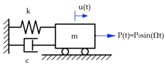
Figure 1.
SDOF structure subjected to dynamic load P(t).
The governing equation of this system is [1]:
where Equation (2) is written with similar connotations to Equation (1). The exact solution to the motion equation of a SDOF system under harmonic load with initial conditions and is the sum of the displacements of the transient state of the system () and the steady state (), and is expressed as [5]:
in which and are defined as:
and
where and are the damping ratio and natural frequency of the system, respectively, and indicates the damped frequency. Finally, is the ratio of the excitation frequency to the system natural frequency.
2.2. Linear Newmark-β Method
One of the most efficient methods of handling equations of motion of SDOF and MDOF systems has been proposed by Newmark [2]. In 1959, Newmark also presented a set of step-by-step numerical equations that are entirely known as the Newmark-β method [5]. In the present study, the linear Newmark-β method is taken into account from [5] to verify the results of the newly developed LGM method.
In order to solve the equation of motion of a MDOF system using the linear Newmark-β method, it is important to remind that the following steps should be generally followed:
- Determination of the initial conditions, , and , where the value of is given by:
- Determination of (assumed time step, e.g., 0.005)
- Determination of the effective stiffness matrix:where and for linear acceleration method.
- Calculation of a and b factors:
- Calculation of the effective load:
- Calculation of displacement, velocity, and acceleration:where,
3. Legendre–Galerkin Matrix Method
Legendre polynomials are among the most important functions in the function approximation theory. The LGM method is highly successful in approximating different functions which mainly stems from the orthogonality of Legendre basis components. This orthogonality makes it easy to find the unknown coefficients of the problem. Another reason for using these basis components is their weight. The weight function will not be a problem for the calculation of the integrals of the Galerkin method and hence the operational matrices of differentiations and other existing functions in the problem can be easily found.
The Galerkin method is an efficient and easy-to-implement approach for solution of the equations of motion of MDOF systems:
under the following initial conditions:
In Equation (14), , and are, respectively, components of mass, damping and stiffness matrices. is the load prescribed at the i-th degree of freedom and and are, respectively, the initial displacement and velocity applied to the i-th degree of freedom. is the displacement of the i-th degree of freedom which is the unknown of the problem, and t represents time.
3.1. Approximation of the Function Using Shifted Legendre Polynomials
- Legendre polynomials: introduced by Lm(t), the Legendre polynomials are defined in the interval [−1, 1] and can be obtained using the following recursive equations:
For further application of these polynomials, they are shifted to the interval [0, L] with the change of variable . Therefore, these shifted polynomials which are shown by are represented as the following:
- Inner product of two functions: the inner product of two functions f(t) and g(t) is represented by . If the functions are known and continuous in the interval [0, b], then:
- Orthogonality of two functions: two functions f(t) and g(t) are orthogonal with respect to the weight function on [a, b] if:
The shifted Legendre polynomials are orthogonal with respect to the weight function in the interval [0, L]. This means that:
Orthogonality of the functions has wide application in the function approximation theory. Any continuous function such as f(x) can be approximated in the interval [0, L] using these polynomials as below:
where fm can be obtained from:
Only the first N + 1 terms of Equation (21) are used in practice. Therefore:
where and are factors of the shifted Legendre vectors expressed as:
3.2. Expression of the LGM Method
Assuming that Equation (14) has a unique solution under the initial conditions in Equation (15), the goal is to find an approximate analytical solution to Equation (14) using the discretized Legendre series as below:
where,
The matrix form of the derivative vector will be:
where is a matrix of dimensions (N + 1) × (N + 1) and is obtained as below:
For example, for different values of N, the following equations are obtained:
Using Equation (27), the k-th derivative of vector is:
Therefore, by replacing and 2 in Equation (29), and then combining the results with Equation (25), one can write:
and
Moreover, the functions can be shown in matrix form as follows:
where is a (N+1) dimensional vector with the following expression:
where,
By introducing Equations (25) and (30)–(32) in Equation (14), it is thus possible to obtain:
Now, let us assume that:
where is an f dimensional vector, A and P are dimensional and M, C and K are the known f × f dimensional matrices, respectively.
Using Equations (35) and (36), the matrix form for approximation of Equation (14) can be obtained as:
or
where,
Equation (38) can be solved using different methods, namely the direct method (i.e., omitting from both sides of the equation and assuming it to vanish), the collocation method, or the Galerkin method.
In the present paper, the Galerkin method is selected to solve the equation. This method tries to minimize the error toward zero with the inner product of the equations in Legendre basis . Consequently:
The above equation is an algebraic system of linear equations with N + 1 equations and N + 1 unknowns that can be easily solved. It is needed, however, to apply the boundary conditions to the problem, as also in accordance with Equation (15). Following Equations (25) and (30), it is:
where,
Finally, in order to find the response of the system in Equation (14) under the initial conditions from Equation (15), by replacing 2f of the rows of Equation (40) with Equation (38), a system of algebraic equations with (N + 1 − 2f) equations (Equation (38)) and 2f equations (Equation (40)) is created. Their solution yields the analytic approximation of the original problem. The last rows of Equation (38) are usually replaced with those equations from Equation (40); however, this is not always obligatory and the rows which will cause the system of equations to be singular can be alternatively replaced.
3.3. Solution of a Calculation Example
Consider the following equation as a SDOF structure without damping under a prescribed load:
The exact solution of this system is:
Choosing N = 5, the LGM method is used to solve the system. The matrix system can be obtained as below:
where and . Furthermore:
where is the shifted Legendre vector on the interval [0,1].
Using the Galerkin matrix method, the following algebraic system of equations is obtained:
Solving the above algebraic equations, the unknown Legendre coefficients are finally obtained as follows:
By replacing the obtained values in Equation (17), the approximate solution for is:
Figure 2 illustrates the results of the exact solution as a function of time, along with its approximation. The accuracy of the LGM method compared to the exact solution can be noticed in the whole time interval.
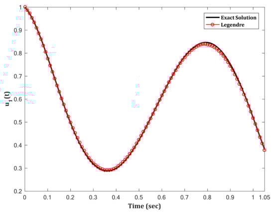
Figure 2.
Comparison of LGM and exact solutions for an SDOF system.
4. Worked Examples and Discussion of Results
For a more exhaustive discussion of the developed LGM method and for a reliable assessment of its potential in structural analysis, the motion equation of an MDOF system is solved in accordance with Equation (14), and some numerical examples are presented. These examples are representative of simple models of real structures (by introducing mass, stiffness, and damping matrices) with and without damping. Accordingly, the current study and the presented formulation of the LGM method represents a first step towards its further extension and use for other applications, such as reliability analysis, optimization, and modal analysis of structures.
4.1. Two-Degree-of-Freedom (2DOF) Structure
A structure with two degrees of freedom (2DOF) is analyzed in different dynamic conditions. The structure is first analyzed under free vibration with no effective damping, and then with additional damping. Successively, the analysis is further performed with the assumption of forced vibration, with and without damping. Basic input data and parameters are summarized as follows:
- Free vibration, without damping: it is , and for mass, damping and stiffness parameters.
The initial conditions are and .
- Free vibration, with damping: it is , while all the other parameters are equal to the undamped case.
The solution of the motion equation using Legendre’s method for and are respectively shown in Figure 3 and Figure 4. Moreover, the LGM results are compared with the exact method, giving evidence of acceptable consistency. It is worth noting that the exact solution is obtained using the Solver of Systems of Equation in the Maple software. Comparisons are then made with the approximate solution.
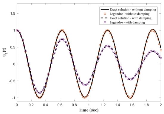
Figure 3.
Free vibration analysis for a 2DOF system. Comparison of as a function of time, as obtained from the LGM method or the exact solution.
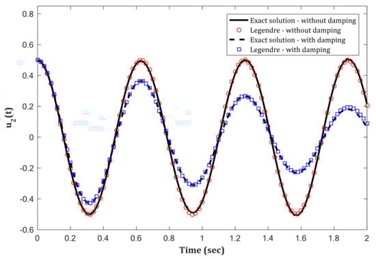
Figure 4.
Free vibration analysis for a 2DOF system. Comparison of as a function of time, as obtained from the LGM method or the exact solution.
Successively, the examined structure is analyzed under forced vibration. In this case, it is:
Once again, the structure is analyzed with and without damping, using the developed LGM method. The analytical results obtained from the LGM method for and are shown in Figure 5 and Figure 6, respectively, and compared with the exact solution, proving again a rather acceptable consistency in the examined time interval.
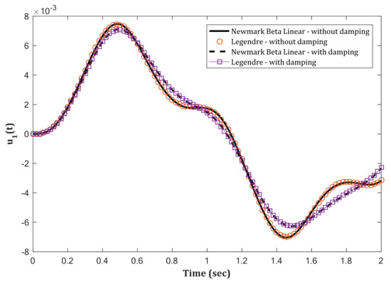
Figure 5.
Forced vibration analysis of a 2DOF system. Comparison of as a function of time, as obtained from the LGM method or the linear Newmark-β method.
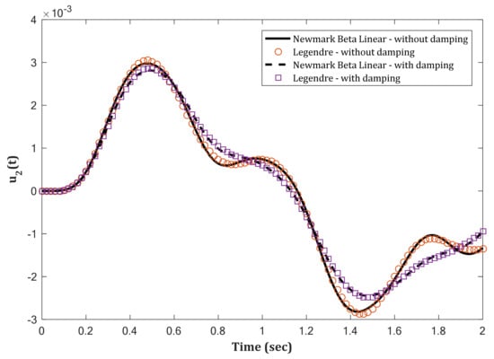
Figure 6.
Forced vibration analysis of a 2DOF system. Comparison of as a function of time, as obtained from the LGM method or the linear Newmark-β method.
4.2. Three-Degree-of-Freedom Structure
As a further validation example, a structure with three degrees of freedom (3DOF) is analyzed in forced and free vibration conditions, with or without damping.
- Free vibration, without damping: it is , and for mass, damping and stiffness, respectively. The initial conditions are and .
- Free vibration, with damping: it is , while the other parameters are the same as without damping.
The results for , and are shown in Figure 7, Figure 8 and Figure 9, respectively, where it is possible to see the comparison of the LGM method and linear Newmark-β method, with rather good consistency.
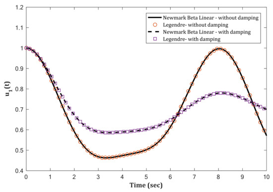
Figure 7.
Free vibration analysis of a 3DOF system. Comparison of as a function of time, as obtained using the LGM method or the linear Newmark-β method.
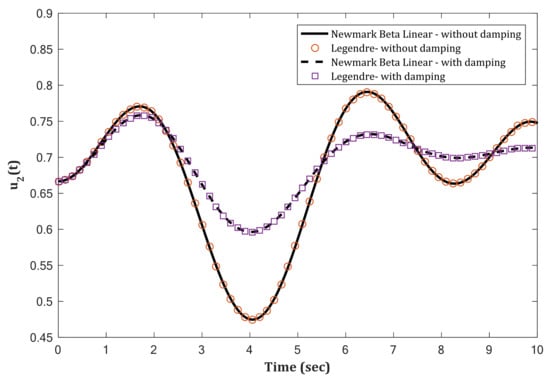
Figure 8.
Free vibration analysis of a 3DOF system. Comparison of as a function of time, as obtained using the LGM method or the linear Newmark-β method.
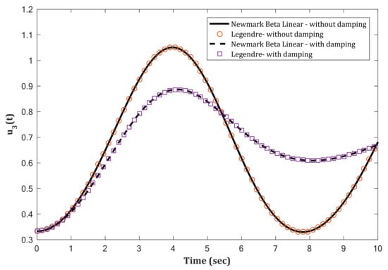
Figure 9.
Free vibration analysis of a 3DOF system. Comparison of as a function of time, as obtained using the LGM method or the linear Newmark-β method.
The equation of motion of the structure under forced vibration (with and without damping) for with initial conditions and is solved further by using Legendre’s method.
The results obtained in this case for , and are proposed in Figure 10, Figure 11 and Figure 12, respectively, and compared with the results by the linear Newmark-β method. Moreover, in this case, the comparative data show the consistency of the LGM with the linear Newmark-β method.
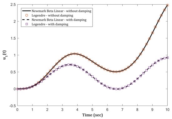
Figure 10.
Forced vibration analysis of a 3DOF system. Comparison of as a function of time, as obtained using the LGM method or the linear Newmark-β method.
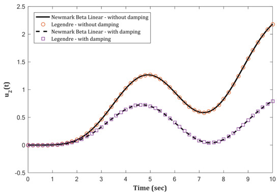
Figure 11.
Forced vibration analysis of a 3DOF system. Comparison of as a function of time, as obtained using the LGM method or the linear Newmark-β method.
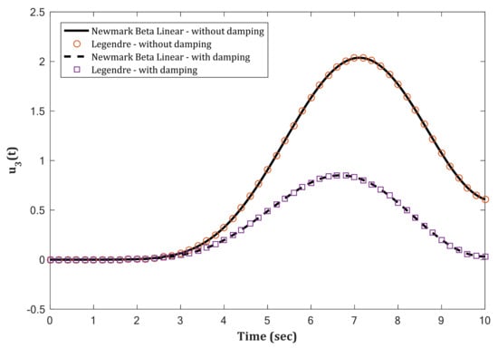
Figure 12.
Forced vibration analysis of a 3DOF system. Comparison of as function of time, as obtained using the LGM method or the linear Newmark-β method.
4.3. Five-Degree-of-Freedom Structure
In conclusion, a structure with five degrees of freedom (5DOF) is analyzed with the LGM method, both under free vibration with and without damping.
- Free vibration, without damping: it is assumed that , and , respectively.
The initial conditions are and .
- Free vibration, with damping: it is assumed that , while the other parameters are the same as in the undamped case.
The solutions of the equation of motion of the structure using the LGM for damped and undamped states, in terms of to , are shown in Figure 13, Figure 14, Figure 15, Figure 16 and Figure 17 and compared with those by the linear Newmark-β method. As for the previously discussed calculation examples, the comparative plots prove an appropriate consistency and a high level of accuracy of the LGM procedure.
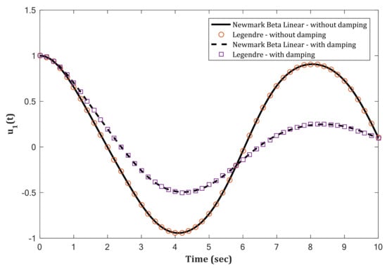
Figure 13.
Free vibration analysis of a 5DOF system. Comparison of as a function of time, as obtained using the LGM method or the linear Newmark-β method.
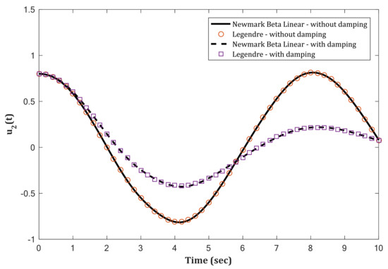
Figure 14.
Free vibration analysis of a 5DOF system. Comparison of as a function of time, as obtained using the LGM method or the linear Newmark-β method.
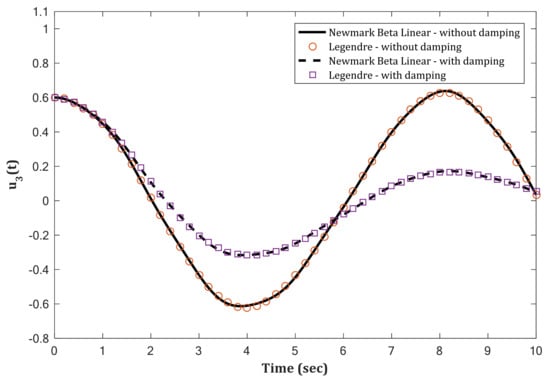
Figure 15.
Free vibration analysis of a 5DOF system. Comparison of as a function of time, as obtained using the LGM method or the linear Newmark-β method.
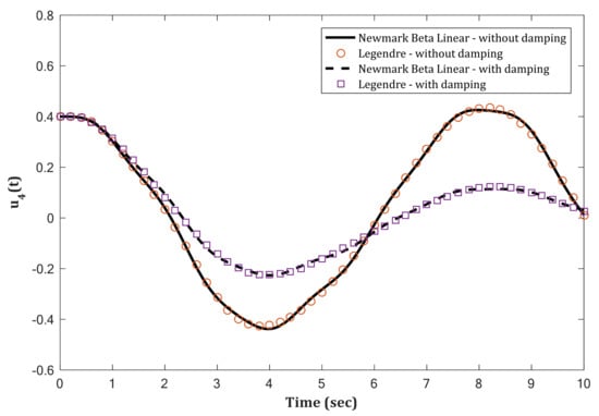
Figure 16.
Free vibration analysis of a 5DOF system. Comparison of as a function of time, as obtained using the LGM method or the linear Newmark-β method.
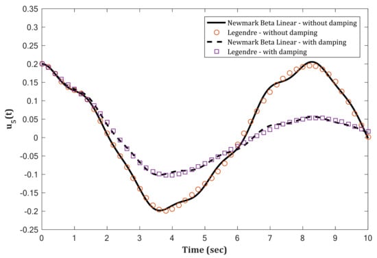
Figure 17.
Free vibration analysis of a 5DOF system. Comparison of as a function of time, as obtained using the LGM method or the linear Newmark-β method.
It should be noted that, in the case of stochastic analysis that is interpreted classically as a repetition of solution for different input values with defined probability density functions (taking into account uncertainties associated with input parameters), the methods such as Monte Carlo simulation (MCS) [60] can be easily used along with the results of LGM method to investigate the problem in a probabilistic manner. This is due to the fact that, in the LGM method, the solution is approximated by discretized Legendre series that can be used as a state function in reliability analysis where no mathematical closed-form state function can be found (e.g., through finite element method). Furthermore, such a solution obtained from the LGM method can also be utilized with analytical reliability methods (e.g., jointly distributed random variables method [61]) or approximate ones (e.g., first and second-order reliability methods (FORM and SORM), point estimate method (PEM), etc. [62]), with less computational efforts in comparison to the MCS method.
5. Conclusions
The Legendre–Galerkin matrix (LGM) method was developed in this study to solve systems of differential equations of motion. As shown, the advantage of this spectral method is that it converts the governing differential equation of a given problem to a system of algebraic equations, based on a set of orthogonal Legendre polynomials. The final solution leads to a good estimate of the solution for a system of differential equations. In the present research study, the selected differential equations were typical of single degree (SDOF) and multi-degree-of-freedom (MDOF) structural systems.
In order to prove the accuracy of the proposed method in the response calculation of SDOF and MDOF structures, a number of numerical examples for damped and undamped structural systems under free or forced vibrations were developed and discussed. When available, exact solutions were taken into account for the comparative analysis of LGM predictions, otherwise, the results of the numerical linear Newmark-β method were used to verify the estimates from the developed LGM method. The overall comparative data showed that the LGM method is of high accuracy in estimating the response of SDOF and MDOF systems and can be thus effectively employed in the solution of fundamental motion equations of structures.
Author Contributions
Conceptualization, M.M., M.R.B., B.J., C.B. and M.A.N.; methodology, M.M., M.R.B.; software, M.M., M.R.B. and C.B.; validation, M.M., M.R.B. and M.A.N.; formal analysis, C.B., M.A.N., M.A.H. and S.M.D.; investigation, C.B., M.A.H., M.A.N. and S.M.D.; writing—original draft preparation, M.M. and B.J.; writing—review and editing, C.B., M.A.N., B.J., S.M.D. and M.A.H.; visualization, M.M., M.R.B., B.J. and C.B.; supervision, C.B., M.A.N., S.M.D. and M.A.H. All authors have read and agreed to the published version of the manuscript.
Funding
This research received no external funding.
Institutional Review Board Statement
Not applicable.
Informed Consent Statement
Not applicable.
Data Availability Statement
Supporting data will be made available upon request.
Conflicts of Interest
The authors declare no conflict of interest.
References
- Chopra, A.K. Dynamics of Structures: Theory and Applications to Earthquake Engineering; Prentice Hall: Hoboken, NJ, USA, 1995; Volume 3. [Google Scholar]
- Newmark, N.M. A method of computation for structural dynamics. J. Eng. Mech. Div. 1959, 85, 67–94. [Google Scholar] [CrossRef]
- Wilson, E.; Farhoomand, I.; Bathe, K. Nonlinear dynamic analysis of complex structures. Earthq. Eng. Struct. Dyn. 1972, 1, 241–252. [Google Scholar] [CrossRef]
- Butcher, J.C. A history of Runge-Kutta methods. Appl. Numer. Math. 1996, 20, 247–260. [Google Scholar] [CrossRef]
- Humar, J. Dynamics of Structures; CRC Press: Boca Raton, FL, USA, 2012. [Google Scholar]
- Clough Ray, W.; Penzien, J. Dynamics of Structures; Computers & Structures Inc.: Berkeley, CA, USA, 1995. [Google Scholar]
- Mason, J.C.; Handscomb, D.C. Chebyshev Polynomials; CRC Press: Boca Raton, FL, USA, 2002. [Google Scholar]
- Dattoli, G.; Ricci, P.E.; Cesarano, C. A note on Legendre polynomials. Int. J. Nonlinear Sci. Numer. Simul. 2001, 2, 365–370. [Google Scholar] [CrossRef]
- Grosswald, E. Bessel Polynomials; Springer: Berlin/Heidelberg, Germany, 2006; Volume 698. [Google Scholar]
- Dattoli, G.; Lorenzutta, S.; Maino, G.; Torre, A.; Cesarano, C. Generalized Hermite polynomials and supergaussian forms. J. Math. Anal. Appl. 1996, 203, 597–609. [Google Scholar] [CrossRef] [Green Version]
- Koekoek, R.; Meijer, H. A generalization of Laguerre polynomials. Siam J. Math. Anal. 1993, 24, 768–782. [Google Scholar] [CrossRef]
- Zhou, J. Differential Transformation and Its Applications for Electronic Circuits; Huazhong Science & Technology University Press: Wuhan, China, 1986. [Google Scholar]
- Odibat, Z.; Momani, S. A generalized differential transform method for linear partial differential equations of fractional order. Appl. Math. Lett. 2008, 21, 194–199. [Google Scholar] [CrossRef] [Green Version]
- Ertürk, V.S.; Momani, S. Solving systems of fractional differential equations using differential transform method. J. Comput. Appl. Math. 2008, 215, 142–151. [Google Scholar] [CrossRef] [Green Version]
- Nazari, D.; Shahmorad, S. Application of the fractional differential transform method to fractional-order integro-differential equations with nonlocal boundary conditions. J. Comput. Appl. Math. 2010, 234, 883–891. [Google Scholar] [CrossRef] [Green Version]
- Alquran, M.T. Applying differential transform method to nonlinear partial differential equations: A modified approach. Appl. Appl. Math. Int. J. 2012, 7, 155. [Google Scholar]
- Fatoorehchi, H.; Abolghasemi, H. Improving the differential transform method: A novel technique to obtain the differential transforms of nonlinearities by the Adomian polynomials. Appl. Math. Model. 2013, 37, 6008–6017. [Google Scholar] [CrossRef]
- Patil, N.; Khambayat, A. Differential transform method for ordinary differential equations. J. Comput. Math. Sci. 2012, 3, 248–421. [Google Scholar]
- Kharrat, B.N.; Toma, G. Differential transform method for solving boundary value problems represented by system of ordinary differential equations of 4 order. World Appl. Sci. J. 2020, 38, 25–31. [Google Scholar]
- Kassem, M.A.; Hemeda, A.; Abdeen, M. Solution of the tumor-immune system by differential transform method. J. Nonli. Sci. Appl. 2020, 13, 9–21. [Google Scholar] [CrossRef] [Green Version]
- Jena, S.K.; Chakraverty, S. Free vibration analysis of Euler–Bernoulli nanobeam using differential transform method. Int. J. Comput. Mater. Sci. Eng. 2018, 7, 1850020. [Google Scholar] [CrossRef]
- Rysak, A.; Magdalena, G. Differential Transform Method as an Effective Tool for Investigating Fractional Dynamical Systems. Appl. Sci. 2021, 11, 6955. [Google Scholar] [CrossRef]
- Najafgholipour, M.; Soodbakhsh, N. Modified differential transform method for solving vibration equations of MDOF systems. Civ. Eng. J. 2016, 2, 123–139. [Google Scholar] [CrossRef] [Green Version]
- El-Shahed, M. Application of differential transform method to non-linear oscillatory systems. Commun. Nonlinear Sci. Numer. Simul. 2008, 13, 1714–1720. [Google Scholar] [CrossRef]
- Momani, S.; Ertürk, V.S. Solutions of non-linear oscillators by the modified differential transform method. Comput. Math. Appl. 2008, 55, 833–842. [Google Scholar] [CrossRef] [Green Version]
- Nourazar, S.; Mirzabeigy, A. Approximate solution for nonlinear Duffing oscillator with damping effect using the modified differential transform method. Sci. Iran. 2013, 20, 364–368. [Google Scholar]
- Chen, C.K.; Ho, S.H. Transverse vibration of a rotating twisted Timoshenko beams under axial loading using differential transform. Int. J. Mech. Sci. 1999, 41, 1339–1356. [Google Scholar] [CrossRef]
- Ho, S.H.; Chen, C.K. Analysis of general elastically end restrained non-uniform beams using differential transform. Appl. Math. Model. 1998, 22, 219–234. [Google Scholar] [CrossRef]
- Özdemir, Ö.; Kaya, M. Flapwise bending vibration analysis of a rotating tapered cantilever Bernoulli–Euler beam by differential transform method. J. Sound Vib. 2006, 289, 413–420. [Google Scholar] [CrossRef]
- Catal, S. Solution of free vibration equations of beam on elastic soil by using differential transform method. Appl. Math. Model. 2008, 32, 1744–1757. [Google Scholar] [CrossRef]
- Arikoglu, A.; Ozkol, I. Vibration analysis of composite sandwich beams with viscoelastic core by using differential transform method. Compos. Struct. 2010, 92, 3031–3039. [Google Scholar] [CrossRef]
- Das, D. The generalized differential transform method for solution of a free vibration linear differential equation with fractional derivative damping. J. Appl. Math. Comput. Mech. 2019, 18, 19–29. [Google Scholar] [CrossRef]
- Bozyigit, B.; Yesilce, Y.; Catal, S. Free vibrations of axial-loaded beams resting on viscoelastic foundation using Adomian decomposition method and differential transformation. Eng. Sci. Technol. Int. J. 2018, 21, 1181–1193. [Google Scholar] [CrossRef]
- Bhrawy, A. An efficient Jacobi pseudospectral approximation for nonlinear complex generalized Zakharov system. Appl. Math. Comput. 2014, 247, 30–46. [Google Scholar] [CrossRef]
- Canuto, C.; Hussaini, M.Y.; Quarteroni, A.; Thomas, A., Jr. Spectral Methods in Fluid Dynamics; Springer Science & Business Media: Heidelberg, Germany, 2012. [Google Scholar]
- Peyret, R. Spectral Methods for Incompressible Viscous Flow; Springer Science & Business Media: Heidelberg, Germany, 2013; Volume 148. [Google Scholar]
- Shen, J.; Tang, T. Spectral and High-Oder Methods with Applications; Science Press: Beijing, China, 2006. [Google Scholar]
- Lucas, T.R.; Reddien, J.; George, W. Some collocation methods for nonlinear boundary value problems. Siam J. Numer. Anal. 1972, 9, 341–356. [Google Scholar] [CrossRef]
- Ortiz, E.L.; Samara, H. An operational approach to the Tau method for the numerical solution of non-linear differential equations. Computing 1981, 27, 15–25. [Google Scholar] [CrossRef]
- Ben-Yu, G. Spectral Methods and Their Applications; World Scientific: Singapore, 1998. [Google Scholar]
- Bernardi, C. Maday Spectral Methods. In The Handbook of Numerical Analysis; Ciarlet, V.P.G., Lions, J.-L., Eds.; Elsevier B.V.: Amsterdam, The Netherlands, 1997. [Google Scholar]
- Bialecki, B.; Karageorghis, A. A Legendre spectral quadrature Galerkin method for the Cauchy-Navier equations of elasticity with variable coefficients. Numer. Algorithms 2017, 77, 491–516. [Google Scholar] [CrossRef]
- Guo, S.; Mei, L.; Li, Y. An efficient Galerkin spectral method for two-dimensional fractional nonlinear reaction–diffusion-wave equation. Comput. Math. Appl. 2017, 74, 2449–2465. [Google Scholar] [CrossRef]
- Mao, Z.; Shen, J. Efficient spectral–Galerkin methods for fractional partial differential equations with variable coefficients. J. Comput. Phys. 2016, 307, 243–261. [Google Scholar] [CrossRef] [Green Version]
- Ren, Q.; Tian, H. Legendre–Galerkin spectral approximation for a nonlocal elliptic Kirchhof-type problem. Int. J. Comput. Math. 2017, 94, 1747–1758. [Google Scholar] [CrossRef]
- Nemati Saray, B. Sparse multiscale representation of Galerkin method for solving linear-mixed Volterra-Fredholm integral equations. Math. Methods Appl. Sci. 2020, 43, 2601–2614. [Google Scholar] [CrossRef]
- Amiri, S.; Hajipour, M.; Baleanu, D. A spectral collocation method with piecewise trigonometric basis functions for nonlinear Volterra–Fredholm integral equations. Appl. Math. Comput. 2020, 370, 124915. [Google Scholar] [CrossRef]
- Zaky, M.A.; Ameen, I.G. A novel Jacob spectral method for multi-dimensional weakly singular nonlinear Volterra integral equations with nonsmooth solutions. Eng. Comput. 2020, 37, 2623–2631. [Google Scholar] [CrossRef]
- Erfanian, M.; Zeidabadi, H.; Mehri, R. Solving Two-Dimensional Nonlinear Volterra Integral Equations Using Rationalized Haar Functions in the Complex Plane. Adv. Sci. Eng. Med. 2020, 12, 409–415. [Google Scholar] [CrossRef]
- Hesameddini, E.; Riahi, M. Bernoulli Galerkin Matrix Method and Its Convergence Analysis for Solving System of Volterra–Fredholm Integro-Differential Equations. Iran. J. Sci. Technol. Trans. A Sci. 2019, 43, 1203–1214. [Google Scholar] [CrossRef]
- Ramadan, M.; Osheba, H.S. A new hybrid orthonormal Bernstein and improved block-pulse functions method for solving mathematical physics and engineering problems. Alex. Eng. J. 2020, 59, 3643–3652. [Google Scholar] [CrossRef]
- Mirzaee, F.; Bimesl, S. A new Euler matrix method for solving systems of linear Volterra integral equations with variable coefficients. J. Egypt. Math. Soc. 2014, 22, 238–248. [Google Scholar] [CrossRef] [Green Version]
- Mirzaee, F. Bernoulli collocation method with residual correction for solving integral-algebraic equations. J. Linear Topol. Algebra 2015, 4, 193–208. [Google Scholar]
- Sahu, P.K.; Ray, S.S. Hybrid Legendre Block-Pulse functions for the numerical solutions of system of nonlinear Fredholm–Hammerstein integral equations. Appl. Math. Comput. 2015, 270, 871–878. [Google Scholar] [CrossRef]
- Pourabd, M. Moving least square for systems of integral equations. Appl. Math. Comput. 2015, 270, 879–889. [Google Scholar]
- Yüzbaşı, Ş. Numerical solutions of system of linear Fredholm–Volterra integro-differential equations by the Bessel collocation method and error estimation. Appl. Math. Comput. 2015, 250, 320–338. [Google Scholar] [CrossRef]
- US DoD. UFC 3-340-02 Structures to Resist the Effects of Accidental Explosions; US DoD: Washington, DC, USA, 2008. [Google Scholar]
- Bounds, W.L. Design of Blast-Resistant Buildings in Petrochemical Facilities; ASCE Publications: Reston, VA, USA, 2010. [Google Scholar]
- Momeni, M.; Hadianfard, M.A.; Bedon, C.; Baghlani, A. Damage evaluation of H-section steel columns under impulsive blast loads via gene expression programming. Eng. Struct. 2020, 219, 110909. [Google Scholar] [CrossRef]
- Hadianfard, M.A.; Malekpour, S.; Momeni, M. Reliability analysis of H-section steel columns under blast loading. Struct. Saf. 2018, 75, 45–56. [Google Scholar] [CrossRef]
- Johari, A.; Momeni, M.; Javadi, A. An analytical solution for reliability assessment of pseudo-static stability of rock slopes using jointly distributed random variables method. Iran. J. Sci. Technol. Trans. Civ. Eng. 2015, 39C2, 351–363. [Google Scholar]
- Nowak, A.S.; Collins, K.R. Reliability of Structures; CRC Press: Boca Raton, FL, USA, 2012. [Google Scholar]
Publisher’s Note: MDPI stays neutral with regard to jurisdictional claims in published maps and institutional affiliations. |
© 2021 by the authors. Licensee MDPI, Basel, Switzerland. This article is an open access article distributed under the terms and conditions of the Creative Commons Attribution (CC BY) license (https://creativecommons.org/licenses/by/4.0/).