A New Foot Trajectory Planning Method for Legged Robots and Its Application in Hexapod Robots

Abstract

Compared with wheeled and tracked robots, legged robots have better movement ability and are more suitable for the exploration of unknown environments. In order to further improve the adaptability of legged robots to complex terrains such as slopes, obstacle environments, and so on, this paper makes a new design of the legged robot’s foot sensing structure that can successfully provide accurate feedback of the landing information. Based on this information, a new foot trajectory planning method named three-element trajectory determination method is proposed. For each leg in one movement period, the three elements are the start point in the support phase, the end point in the support phase, and the joint angle changes in the transfer phase where the first two elements are used to control the height, distance, and direction of the movement, and the third element is used make decisions during the lifting process of the leg. For the support phase, the trajectory is described in Cartesian space, and a spline of linear function with parabolic blends is used. For the transfer phase, the trajectory is described in joint-space, and the joint angle function is designed as the superposition of the joint angle reverse-chronological function and the interpolation function which is obtained based on joint angle changes. As an important legged robot, a hexapod robot that we designed by ourselves with triangle gait is chosen to test the proposed foot trajectory planning method. Experiments show that, while the foot’s landing information can be read and based on the three-element trajectory planning method, the hexapod robot can achieve stable movement even in very complex scenes. Although the experiments are performed on a hexapod robot, our method is applicable to all forms of legged robots.

1. Introduction

With the development of AI technology, mobile robots are appearing more and more frequently in public. According to the motion mode, mobile robots can be divided into wheeled robots [1,2], tracked robots [3], and legged robots [4,5]. In the face of complex environments as well as rugged terrains, legged robots have incomparable flexibility and applicability compared with the other two kinds of robots.

The design idea of legged robots originated from bionics. Inspired by mammals, insects, amphibians, etc., legged robots try to imitate the structure as well as movement mode of different legs [6]. Up to this point, there have been many different kinds of bionic legged robots that were designed and studied. With the support of the U.S. Department of Defense and by imitating a dog, Boston Dynamics developed the quadruped robot BigDog, which possessed strong obstacle crossing ability and could overcome rugged terrain [7]. Inspired by insects, Case Western Reserve University designed a bionic insect robot that could jump, walk, turn, and avoid obstacles in a certain space [8]. In China, also from the perspective of bionics and combining motion control analysis, different kinds of legged robots were designed by Shandong University [9,10], Harbin University of Science and Technology [11], and Shanghai Jiaotong University [12].

Common legged robots include biped robots, quadruped robots, hexapod robots, and octopod robots. For biped robots , the movement balance is difficult to control [13,14]. Even very simple walking similar to those in humans will become a big challenge for biped robots . For quadruped robots, they are able to walk steadily, but have strong dependencies on each leg [15]. When one of the four legs breaks for some reason, the quadruped robot cannot continue working anymore. In contrast, hexapod robots can still adjust in the case that one leg breaks through an adaptive fault tolerant gait [16]. Up to this point, there is very little work about octopod robots in terms of complex control [17]. All in all, hexapod robots have natural advantages in movement stability and are studied a lot.

In terms of the hexapod robot’s stable movement in different terrains, most research realized this by switching gait. Bai et al. presented a novel CPG (center pattern generator)-based gait generation for a curved-leg hexapod robot and enabled the robot to achieve smooth and continuous mutual gait transitions [18]. Ouyang presented an adaptive locomotion control approach for a hexapod robot by using a 3D two-layer artificial center pattern generator (CPG) network [19]. These methods all obtained promising results in some aspects, but they could not confront any complex scene because of the limited gait patterns. Our current work, from another point of view, finds a new method to help the hexapod robot improve its movement stability for all kinds of terrains, which is achieved by adaptively planning the foot’s trajectory in order to stabilize the robot’s attitude. With this method, the gait can remain the same.

To implement the above theory on a physical robot, the robot should have the ability to sense its landing information firstly. In [20], Zha et al. developed a new kind of free gait controller and applied it to a large-scale hexapod robot with heavy load, where sensory feedback signals of the foot position were employed in both the free gait planner and the gait regulator. In [21], Faigl and Čížek presented a minimalistic approach for a hexapod robot’s adaptive locomotion control, which enabled traversing rough terrains with a small and affordable hexapod walking robot, and servomotor position feedback was also used to reliably detect the ground contact point. Up to this point, the problem of how to obtain landing information has not been sufficiently considered as well as studied in most legged robots. In [21], this information was obtained by comparing the joint error and the error threshold. In some other works, based on the robot’s dynamic model, joint torque feedback was selected to judge whether the feet had touched the ground [22]. However, the sensors used for such joint torque feedback are always with large volume and high in terms of price, which limits their utility in small robots. To solve these lingering issues, we create a new design of the legged robot’s foot by adding a short-stroke inching button in order to obtain accurate feedback of the foot’s landing information. By conducting experiments on our designed robot in real environments, this foot sensing structure is proved to be easy to use, with low cost and strong sensitivity.

The rest of the paper is structured as follows. Section II introduces the hexapod robot we designed in detail, including its mechanical structure and electrical structure, especially the new design of the robot’s foot sensing structure. To elucidate our method, the robot’s mathematic model is firstly given in section III. All details of the foot trajectory planning method including simulation verification are in Section IV. Section V provides the method’s application in a triangle gait. Section VI shows the experiment results. Conclusions are finally put forward in Section VII.

2. The Hexapod Robot

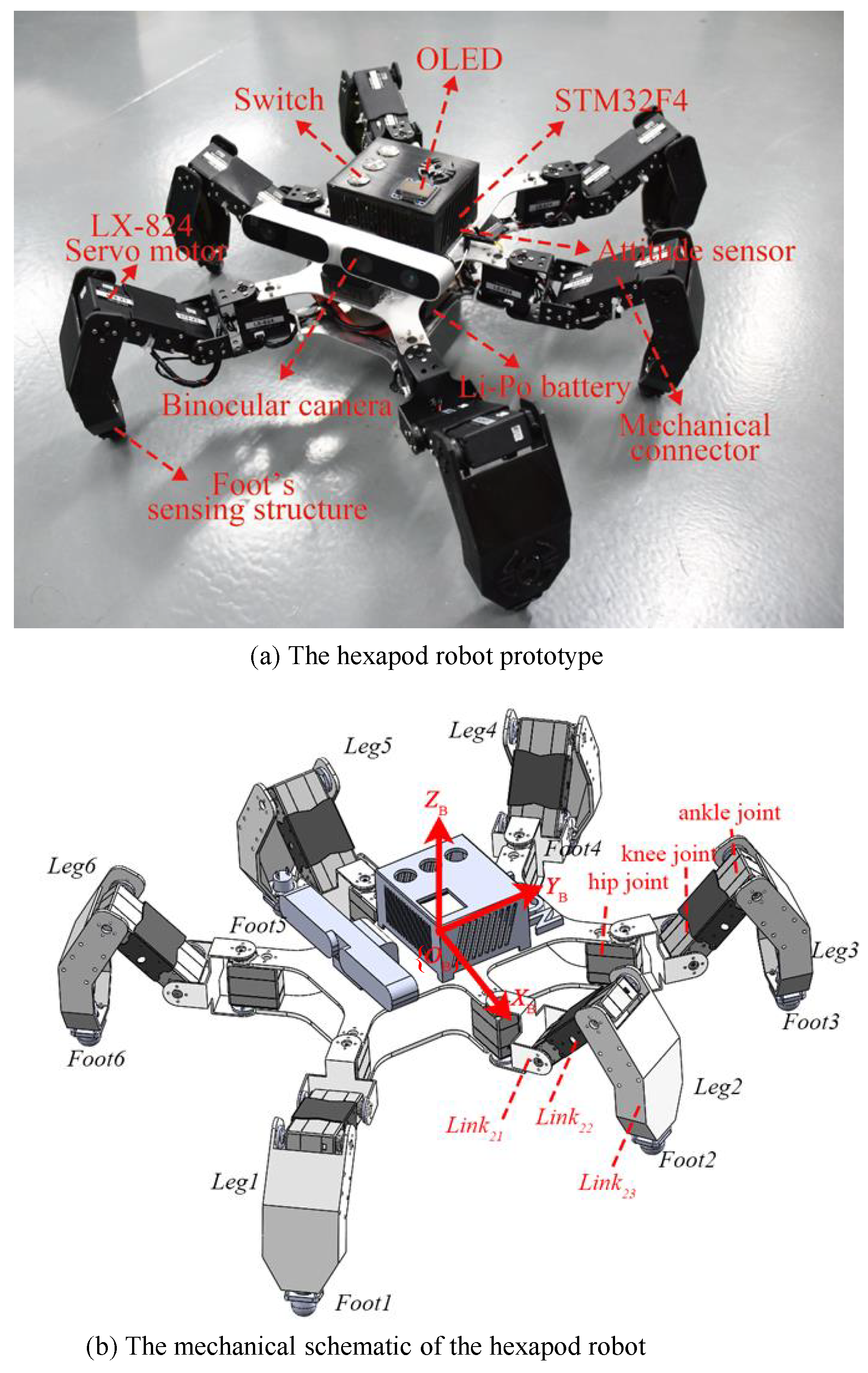
The robot we designed is as shown in Figure 1, where (a) is the hexapod robot prototype, and (b) is its mechanical schematic. For the sake of description, the six legs are numbered as $Leg1$ to $Leg6$ in a counter-clockwise fashion.

2.1. The Hexapod Robot’s Mechanical Structure

From the perspective of mechanical structure, the hexapod robot is mainly composed of a body, legs, and feet. Normally, to better guarantee the stability and controllability, the hexapod robot is centrally symmetric.

2.1.1. The Body

For our hexapod robot, its body is composed of two identical plates with the length and width ratio of 2:1. These two plates are placed up and down and are fixedly connected by the hip joints of six legs. Located between the two plates is the battery. The STM32F4 microcontroller, binocular camera and attitude sensor are placed on the top of the upper plate.

2.1.2. The Leg

As in Figure 1b, for each leg, there are three joints from the direction of body to foot tip, which are the hip joint, the knee joint, and the ankle joint. Different joints are connected by links named as $Lin{k}_{i1}$ (between the hip joint and the knee joint), $Lin{k}_{i2}$ (between the knee joint and the ankle joint), and $Lin{k}_{i3}$ (between the ankle joint and the foot tip) for the $ith$ leg. For the hexapod robot, the total of 18 degrees of freedom is utilized.

2.1.3. The Foot

To help the robot to sense its foot landing information, this paper creates a new design of the legged robot’s foot sensing structure as in Figure 2. A short-stroke inching button is used here. Once one foot touches the ground, the reaction force from the ground will press the short-stroke inching button, and then landing information will be transferred to the controller. When the foot is lifted off the ground, the button is reset and prepares for the next landing. A hemispherical foot tip is designed to ensure that the short-stroke inching button can be pressed regardless of the direction of the foot’s fall.

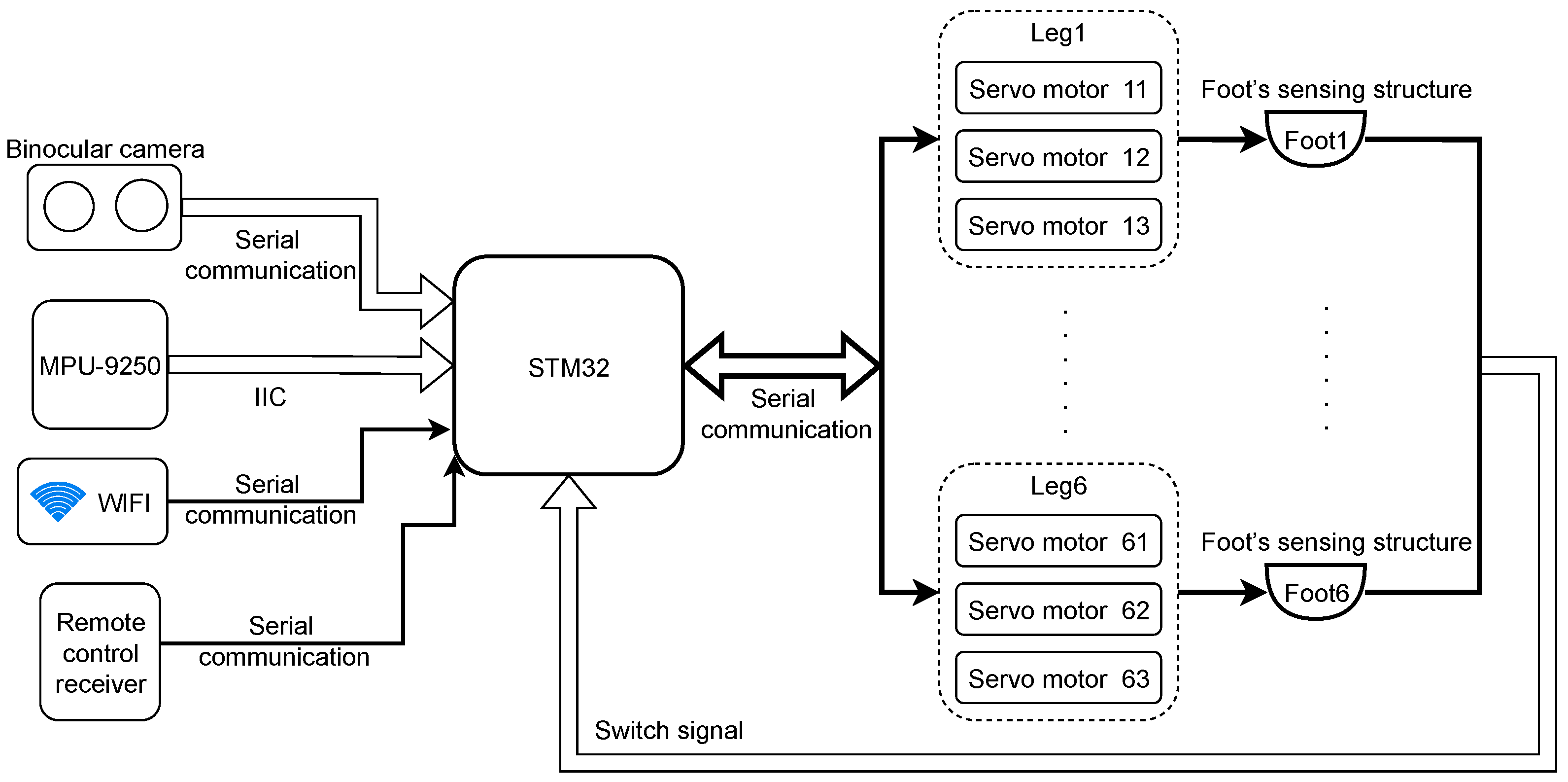
2.2. The Hexapod Robot’s Electrical Structure

The hexapod robot’s electrical structure is shown in Figure 3.

The sensory unit includes five parts as follows.

(1) Binocular camera for object capture and tracking.

(2) Attitude sensor MPU-9250 for measuring the robot’s posture. MPU-9250 is a System in Package (SiP) and contains a 3-axis gyroscope, a 3-axis accelerometer, and AK8963, a 3-axis digital compass. As accelerometers and magnetometers have high frequency noise while the gyroscope has low frequency noise, by utilizing their complementary characteristics in frequency and fusing the low-pass filtered accelerometer and magnetometer data with high-pass filtered gyroscope data, the attitude feedback information with high precision can be obtained.

(3) WIFI module for remote data transmission.

(4) Remote control receiver for instructions receiving.

(5) Foot sensing structure for landing information.

The control unit is STM32, and it outputs the commands to the motion unit, more specifically, the 18 servo motors through serial ports. For each leg, its three servo motors cooperate with each other in a certain time sequence and finally achieve the foot to reach the specified point in space.

The hexapod robot’s technical specifications are provided in

Table 1. Technical specifications of the hexapod robot prototype.

Structure	Parameters
		Value	Unit
Servo motor	Number	18	\
	Weight	57.0	g
Power supply	Voltage	7.4	DC(V)
Body	Length	254.1	mm
	Width	179.3	mm
	Height	3.0	mm
Leg $Lin{k}_{i1}$	Length	45.5	mm
	Weight	18.8	g
Leg $Lin{k}_{i2}$	Length	75.0	mm
	Weight	14.7	g
Leg $Lin{k}_{i3}$	Lenght	109.6	mm
	Weight	41.1	g
Foot	Radius	9.5	mm
	Lenght	19.5	mm
	Weight	6.3	g

.

3. Hexapod Robot Kinematics Modeling

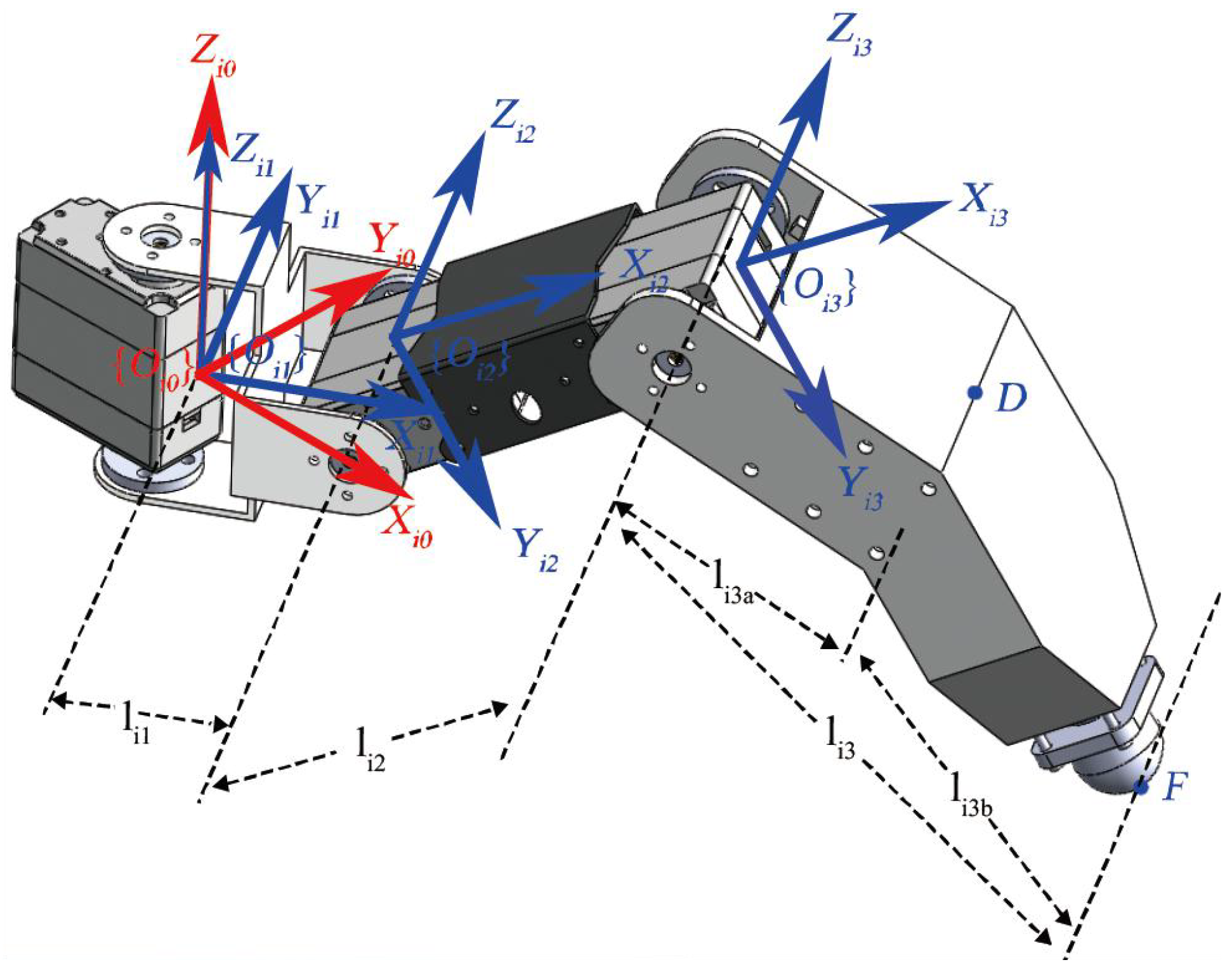
The robot’s kinematic model can help us quantitatively analyze the robot’s velocity, acceleration, attitude, and so on from a mathematical point of view. To establish the kinematic model of the hexapod robot, for each leg i, three coordinates are defined at the hip joint ($\left\{O_{i1}\right\}$), the knee joint ({$O_{i2}$}), and the ankle joint ({$O_{i3}$}), respectively, as depicted in Figure 4. The reference coordinate is $\left\{O_{i0}\right\}$. For each coordinate $\left\{O_{ij}\right\}(i=1,\cdots ,6;j=1,\cdots ,3)$, the $Z_{ij}$ axis coincides with the axis of the jth joint. The $X_{ij}$ axis is the common perpendicular between the axes of the jth joint and the $(j+1)$th joint. The $Y_{ij}$ axis is then determined according to the right-hand rule. In this paper, the kinematic model is based on the DH (Denavit–Hartenberg) method [23], and the parameters are provided in

Table 2. Denavit-Hartenberg parameters.

Joint j	${\mathit{\alpha }}_{\mathit{j}-1}$	${\mathit{a}}_{\mathit{j}-1}$	${\mathit{d}}_{\mathit{j}}$	${\mathit{\theta }}_{\mathit{j}}$
1	0	0	0	${\theta }_1$
2	$-\pi$/2	$l_{i1}$	0	${\theta }_2$
3	0	$l_{i2}$	0	${\theta }_3$

. Since the six legs are the same, we do not distinguish the leg number i anymore, and only the joint number j is considered in the description that follows.

The relative translations and rotations between the $(j-1)$th and the jth joint coordinates are computed by the transformation matrix (1).

$${}_j^{j-1}T=\left[\begin{array}{cccc}cos{\theta }_j& -sin{\theta }_j& 0& a_{j-1}\\ sin{\theta }_{j}cos{\alpha }_{j-1}& cos{\theta }_{j}cos{\alpha }_{j-1}& -sin{\alpha }_{j-1}& -sin{\alpha }_{j-1}{d}_j\\ sin{\theta }_{j}sin{\alpha }_{j-1}& cos{\theta }_{j}sin{\alpha }_{j-1}& cos{\alpha }_{j-1}& cos{\alpha }_{j-1}{d}_j\\ 0& 0& 0& 1\end{array}\right].$$

(1)

3.1. The Forward Kinematics

Based on (1), the transformation matrix from the coordinate $\left\{O_{i3}\right\}$ to $\left\{O_{i0}\right\}$ is the following.

$$\begin{array}{ll}{}_3^{0}T\hfill & ={}_1^{0}T{}_2^{1}T{}_3^{2}T\\ & =\left[\begin{array}{cccc}cos{\theta }_1& -sin{\theta }_1& 0& 0\\ sin{\theta }_1& cos{\theta }_1& 0& 0\\ 0& 0& 1& 0\\ 0& 0& 0& 1\end{array}\right]\left[\begin{array}{cccc}cos{\theta }_2& -sin{\theta }_2& 0& l_{i1}\\ 0& 0& 1& 0\\ -sin{\theta }_2& -cos{\theta }_2& 0& 0\\ 0& 0& 0& 1\end{array}\right]\left[\begin{array}{cccc}cos{\theta }_3& -sin{\theta }_3& 0& l_{i2}\\ sin{\theta }_3& cos{\theta }_3& 0& 0\\ 0& 0& 1& 0\\ 0& 0& 0& 1\end{array}\right]\hfill \\ & =\left[\begin{array}{cccc}cos({\theta }_2+{\theta }_3)cos{\theta }_1& -sin({\theta }_2+{\theta }_3)cos{\theta }_1& -sin{\theta }_1& cos{\theta }_1(l_{i1}+l_{i2}cos{\theta }_2)\\ cos({\theta }_2+{\theta }_3)sin{\theta }_1& -sin({\theta }_2+{\theta }_3)sin{\theta }_1& cos{\theta }_1& sin{\theta }_1(l_{i1}+l_{i2}cos{\theta }_2)\\ -sin({\theta }_2+{\theta }_3)& -cos({\theta }_2+{\theta }_3)& 0& -l_{i2}sin{\theta }_2\\ 0& 0& 0& 1\end{array}\right].\hfill \end{array}$$

(2)

The coordinate of the foot tip with respect to the coordinate $\left\{O_{i3}\right\}$ is the following.

$${}^3{P}_F={\left[\begin{array}{cccc}{x}_{\left\{O_{i3}\right\}}& y_{\left\{O_{i3}\right\}}& z_{\left\{O_{i3}\right\}}& 1\end{array}\right]}^T.$$

(3)

Then, the coordinate of the foot tip with respect to the coordinate $\left\{O_{i0}\right\}$ is described in Equation (4).

$$\begin{array}{ll}{}^0{P}_F\hfill & ={}_3^{0}T{}^3{P}_F\\ & =\left[\begin{array}{c}cos{\theta }_1(l_{i1}+l_{i2}cos{\theta }_2)-z_{\left\{O_{i3}\right\}}sin{\theta }_1+x_{\left\{O_{i3}\right\}}cos({\theta }_2+{\theta }_3)cos{\theta }_1-y_{\left\{O_{i3}\right\}}sin({\theta }_2+{\theta }_3)cos{\theta }_1\\ z_{\left\{O_{i3}\right\}}cos{\theta }_1+sin{\theta }_1(l_{i1}+l_{i2}cos{\theta }_2)+x_{\left\{O_{i3}\right\}}cos({\theta }_2+{\theta }_3)sin{\theta }_1-y_{\left\{O_{i3}\right\}}sin({\theta }_2+{\theta }_3)sin{\theta }_1\\ -y_{\left\{O_{i3}\right\}}cos({\theta }_2+{\theta }_3)-x_{\left\{O_{i3}\right\}}sin({\theta }_2+{\theta }_3)-l_{i2}sin{\theta }_2\\ 1\end{array}\right].\hfill \end{array}$$

(4)

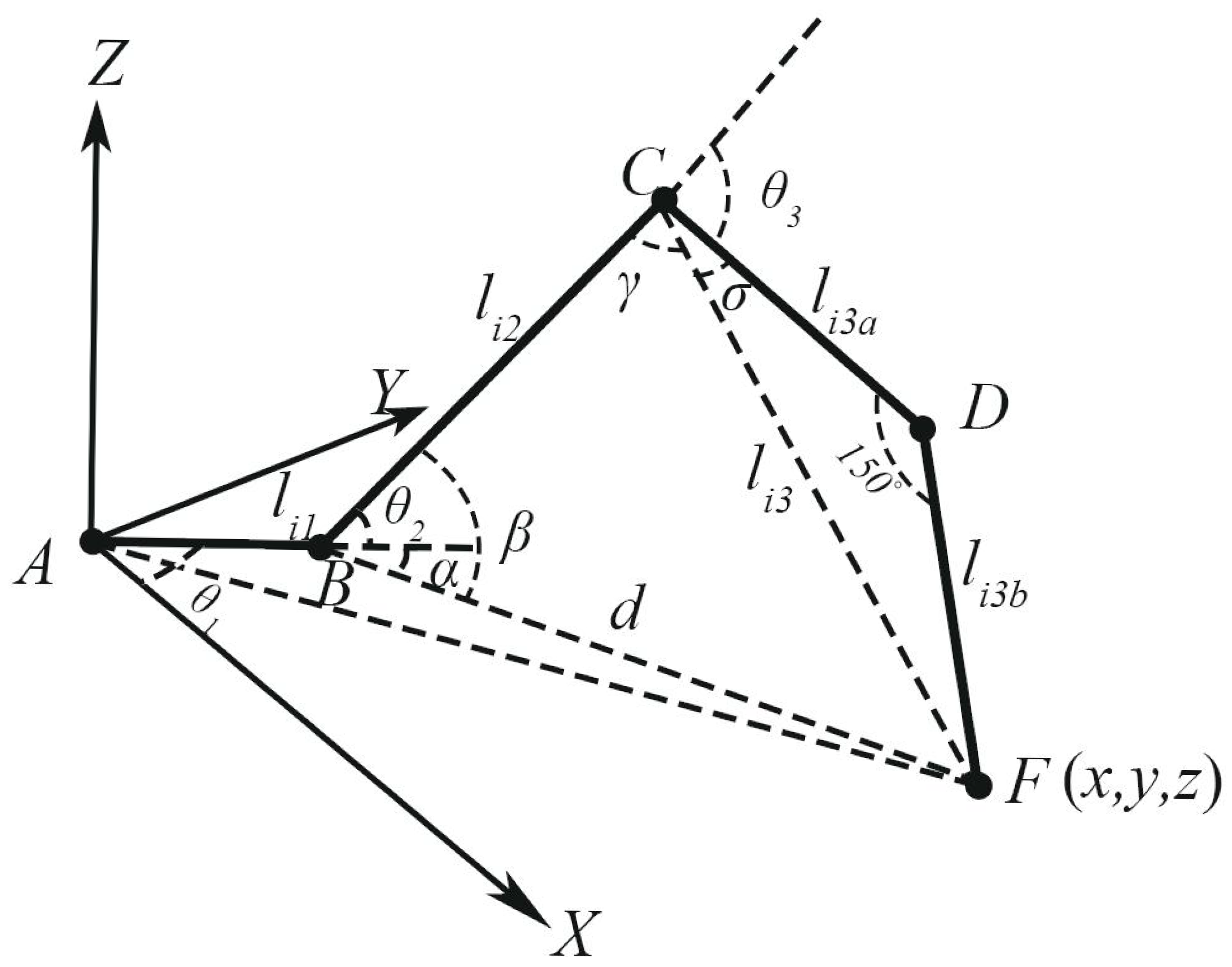
3.2. The Inverse Kinematics

A geometric method is used in this work for the inverse kinematics analysis. It is intuitive and clear, and the solution can be simultaneously unique by restricted conditions. The leg’s diagram for the solution to its inverse kinematics is shown in Figure 5. The angle of CDF is ${150}^{\circ }$, resulting from the robot leg’s fixed mechanical structure design, as shown in Figure 1 and Figure 4. Based on this diagram and by combing geometric knowledge, we have the following.

$$d=\sqrt{{(\sqrt{x^2+y^2}-l_{i1})}^2+z^2},$$

(5)

$$l_{i3}=\sqrt{{l_{i3a}}^2+{l_{i3b}}^2-2l_{i3a}{l}_{i3b}cos\frac{5\pi }{6}},$$

(6)

$$cos\beta =\frac{d^2+{l_{i2}}^2-{l_{i3}}^2}{2l_{i2}d},$$

(7)

$$cos\gamma =\frac{{l_{i2}}^2+{l_{i3}}^2-d^2}{2l_{i2}{l}_{i3}},$$

(8)

$$cos\sigma =\frac{{l_{i3}}^2+{l_{i3a}}^2-{l_{i3b}}^2}{2l_{i3}{l}_{i3a}},$$

(9)

$$sin\alpha =\frac{-z}{d}.$$

(10)

Thus, the inverse kinematics can be easily obtained as follows.

$$\left\{\begin{array}{c}{\theta }_1=arctan\frac{y}{x},\hfill \\ {\theta }_2=\beta -\alpha =arccos\frac{d^2+{l_{i2}}^2-{l_{i3}}^2}{2l_{i2}d}+arcsin\frac{z}{d},\hfill \\ {\theta }_3=\pi -\gamma -\sigma \hfill \\ =\pi -arccos\frac{{l_{i2}}^2+{l_{i3}}^2-d^2}{2l_{i2}{l}_{i3}}-arccos\frac{{l_{i3}}^2+{l_{i3a}}^2-{l_{i3b}}^2}{2l_{i3}{l}_{i3a}}.\hfill \end{array}\right.$$

(11)

4. The Three-Element Trajectory Determination Method

For a hexapod robot, planning its foot trajectory is very important, and it will affect the robot’s flexibility and stability. While moving, the robot’s leg may be in the support phase in order to drive the robot towards a certain direction or off the ground and in the transfer phase. The gait is then realized by switching between the support phase and transfer phase in different sequences. For each leg, its trajectory planning is worth studying in order to enrich the movement of legged robots.

In this paper, we design a three-element trajectory determination method to help the robot plan its foot’s movement. The three elements used are the start point in support phase $P_0=(x_0,y_0,z_0)$, the end point in support phase $P_1=(x_1,y_1,z_1)$, and the joint angle changes in transfer phase $\Delta \theta =[\Delta {\theta }_1,\Delta {\theta }_2,\Delta {\theta }_3]$. $P_0$ and $P_1$ are used to control the height, distance, and the direction of the movement, while $\Delta \theta$ is used to make decisions on the lifting motion of the leg. Applying this method to legged robots, this paper transfers the six variables of $P_0$ and $P_1$ to another three variables that are related to the movement of legged robots, which are height, direction, and distance. Such a transfer is based on some restrictions such as symmetry, equal altitude, vertical landing, etc. $\Delta \theta$ is set according to the feedback information from the foot. The trajectory planning methods in the support phase and transfer phase are different, and they are elaborated separately.

4.1. Trajectory Planning in Support Phase

By using MATLAB, Figure 6 simulates the trajectory planning process in the support phase, where $J_1$, $J_2$, and $J_3$ represent the hip joint, the knee joint, and the ankle joint, respectively, while $J_5$ represents the foot tip. $J_4$ is fixed in $Lin{k}_{i3}$. In Figure 6a, $P_0$ and $P_1$ are the start point and the end point of the foot, while $O_0$ and $O_1$ are the start point and the end point of the hip joint in Figure 6b.

Traditionally, during the hexapod robot’s movement, the angles of the knee joint $J_2$ and the ankle joint $J_3$ are always fixed and not considered. Then, based on the forward kinematics model, the foot will rotate around the hip joint $J_1$, and its trajectory is $\stackrel{{\displaystyle ⁔}}{P_0{P}_1}$, as shown in Figure 6a. When the foot is on the ground, the body needs to move forward with the foot $J_5$ as the fulcrum, and the joint $J_1$ will then move along the trajectory $\stackrel{{\displaystyle ⁔}}{O_0{O}_1}$, as shown in Figure 6b. As the relative position of the hip joint to the robot’s body center remains unchanged, the center of the robot will also move according to $\stackrel{{\displaystyle ⁔}}{O_0{O}_1}$, which means the robot will shake. Therefore, to ensure accuracy in direction as well as stability while moving, the hexapod robot’s foot trajectory in the support phase should better be a straight line $\overline{P_0{P}_1}$, as shown in Figure 6a. Then, $J_1$ will move along $\overline{O_0{O}_1}$, as shown in Figure 6b. Here, the robot’s moving direction keeps constant to ensure that the robot moves in a straight line.

According to the inverse kinematics model, the foot’s trajectory in straight line is planned in Cartesian space. To ensure the robot’s speed, the trajectory’s continuity, and the servo motor’s angular velocity, a spline of linear function with parabolic blends is used in (12).

$$F\left(t\right)=\left\{\begin{array}{cc}{a}_f{t}^2+b_{f}t+c_f,& 0\le t\le T_b;\\ k_{f}t+d_f,& T_b<t\le T_f-T_b;\\ e_f{t}^2+m_{f}t+n_f,& T_f-T_b<t\le T_f.\end{array}\right.$$

(12)

$F\left(t\right)$ can be $X\left(t\right)$, $Y\left(t\right)$, and $Z\left(t\right)$, which are the foot’s coordinates in X axis, Y axis, and Z axis, respectively. $a_f$ to $n_f$ are the parameters, and they are different for different axes. $T_b$ is the movement time of the parabola phase, and it is the same for $X\left(t\right)$, $Y\left(t\right)$, and $Z\left(t\right)$ in order to guarantee the stabilization of movement acceleration. $T_f$ is the time of the total support phase. Some restricted conditions are set at the same time in (13).

$$\left\{\begin{array}{c}\underset{t\to {T_b}^{-}}{lim}F\left(t\right)=\underset{t\to {T_b}^{+}}{lim}F\left(t\right),\hfill \\ \underset{t\to {T_b}^{-}}{lim}{F}^{\prime }\left(t\right)=\underset{t\to {T_b}^{+}}{lim}{F}^{\prime }\left(t\right),\hfill \\ \underset{t\to {(T_f-T_b)}^{-}}{lim}F\left(t\right)=\underset{t\to {(T_f-T_b)}^{+}}{lim}F\left(t\right),\hfill \\ \underset{t\to {(T_f-T_b)}^{-}}{lim}{F}^{\prime }\left(t\right)=\underset{t\to {(T_f-T_b)}^{+}}{lim}{F}^{\prime }\left(t\right),\hfill \\ F^{\prime }\left(0\right)=0,\hfill \\ F^{\prime }\left(T_f\right)=0.\hfill \end{array}\right.$$

(13)

Take $X\left(t\right)$ as an example, as $P_0=(x_0,y_0,z_0)$ and $P_1=(x_1,y_1,z_1)$; according to (13), we have the following.

$$\left\{\begin{array}{c}X\left(0\right)=c_x=x_0,\hfill \\ X\left(T_f\right)=e_x{T_f}^2+m_x{T}_f+n_x=x_1.\hfill \end{array}\right.$$

(14)

By combining all of the restricted conditions, we have the following.

$$\left\{\begin{array}{c}{a}_x{T_b}^2+b_x{T}_b+c_x=k_x{T}_b+d_x,\hfill \\ \frac{1}{2}{a}_x{T}_b+b_x=k_x,\hfill \\ e_x{(T_f-T_b)}^2+m_x(T_f-T_b)+n_x=k_x(T_f-T_b)+d_x,\hfill \\ \frac{1}{2}{e}_x(T_f-T_b)+m_x=k_x,\hfill \\ b_x=0,\hfill \\ \frac{1}{2}{e}_x{T}_f+m_x=0.\hfill \end{array}\right.$$

(15)

For a given robot, when $T_b$ and $T_f$ are set, the equations above can be solved. The same can be performed for $Y\left(t\right)$ and $Z\left(t\right)$, and the trajectory of the foot in support phase can be obtained and is defined as $G\left(t\right)=\left[X\right(t),Y(t),Z(t\left)\right]$. According to the inverse kinematics model in (11), the angle function of the three joints can be obtained and is defined as ${\theta }_{\mathrm{S}}\left(t\right)=[{\theta }_1\left(t\right),{\theta }_2\left(t\right),{\theta }_3\left(t\right)]$.

4.2. Trajectory Planning in Transfer Phase

Transfer phase is the phase when the foot is in the air and moves from the end point of one movement period to the start point of the next movement period. Compared with support phase, the transfer phase has fewer restrictions. The only requirement is that the foot should complete its trajectory in time $T_f$.

The trajectory planning in transfer phase is performed in joint-space. Considering computational simplicity as well as the trajectory’s reliability, this paper designs trajectory planning to occur in this phase as the superposition of two functions: one is what we call the joint angle reverse-chronological function and the other is the joint angle changes interpolation function.

4.2.1. Joint Angle Reverse-Chronological Function

We named it as reverse-chronological function because the trajectory planned based on this function is symmetrical with the trajectory in the support phase along the time $t=T_f$. As it is planned in joint-space, we provide the joint angle reverse-chronological function as Equation (16).

$${\theta }_{\mathrm{B}}\left(t\right)={\theta }_{\mathrm{S}}(2T_f-t)=[{\theta }_1(2T_f-t),{\theta }_2(2T_f-t),{\theta }_3(2T_f-t)].$$

(16)

4.2.2. Joint Angle Changes Interpolation Function

The joint angle changes interpolation function is defined as ${\theta }_{\mathrm{P}}\left(t\right)=[{\theta }_{\mathrm{P}\_1}\left(t\right),{\theta }_{\mathrm{P}\_2}\left(t\right),{\theta }_{\mathrm{P}\_3}\left(t\right)]$, where ${\theta }_{\mathrm{P}\_j}\left(t\right),(j=1,2,3)$ is the angle changes interpolation function for the $jth$ joint. Considering the continuity of the velocity as well as the acceleration, for each joint, ${\theta }_{\mathrm{P}\_j}\left(t\right)$ is a quartic polynomial, as described in Equation (17):

$${\theta }_{\mathrm{P}\_j}\left(t\right)=a_4{t}^4+a_3{t}^3+a_2{t}^2+a_{1}t+a_0.$$

(17)

where $a_0$ to $a_4$ are the parameters of ${\theta }_{\mathrm{P}\_j}\left(t\right)$ and will be different according to different joints.

To ensure the continuity of the joint angle, the joint angle changes at the start and end time should be zero. To ensure the stability of the joint rotation, the velocity of the joint angle changes at the start, and the end time should also be zero.

$$\left\{\begin{array}{c}{\theta }_{\mathrm{P}\_j}\left(t\right)\left(T_f\right)=0,\hfill \\ {\theta }_{\mathrm{P}\_j}\left(t\right)\left(2T_f\right)=0,\hfill \\ {\theta }_{\mathrm{P}\_j}{\left(t\right)}^{\prime }\left(T_f\right)=0,\hfill \\ {\theta }_{\mathrm{P}\_j}{\left(t\right)}^{\prime }\left(2T_f\right)=0.\hfill \end{array}\right.$$

(18)

To realize the symmetry of the angle changes, we hope that ${\theta }_{\mathrm{P}\_j}\left(t\right)$ arrives at the set joint angle change $\Delta {\theta }_j$ at the middle time of this phase; thus, we have the following.

$${\theta }_{\mathrm{P}\_j}\left(\frac{3}{2}{T}_f\right)=\Delta {\theta }_j.$$

(19)

Then, the relationship matrices (20) and (21) can be obtained as follows.

$$\left[\begin{array}{c}0\\ \Delta {\theta }_j\\ 0\\ 0\\ 0\end{array}\right]=\left[\begin{array}{ccccc}{T_f}^4& {T_f}^3& {T_f}^2& T_f& 1\\ {\left(\frac{3}{2}{T}_f\right)}^4& {\left(\frac{3}{2}{T}_f\right)}^3& {\left(\frac{3}{2}{T}_f\right)}^2& \frac{3}{2}{T}_f& 1\\ {\left(2T_f\right)}^4& {\left(2T_f\right)}^3& {\left(2T_f\right)}^2& 2T_f& 1\\ 4{T_f}^3& 3{T_f}^2& 2T_f& 1& 0\\ 4{\left(2T_f\right)}^3& 3{\left(2T_f\right)}^2& 2\left(2T_f\right)& 1& 0\end{array}\right]\left[\begin{array}{c}{a}_4\\ a_3\\ a_2\\ a_1\\ a_0\end{array}\right].$$

(20)

$$\left[\begin{array}{c}{a}_4\\ a_3\\ a_2\\ a_1\\ a_0\end{array}\right]={\left[\begin{array}{ccccc}{T_f}^4& {T_f}^3& {T_f}^2& T_f& 1\\ {\left(\frac{3}{2}{T}_f\right)}^4& {\left(\frac{3}{2}{T}_f\right)}^3& {\left(\frac{3}{2}{T}_f\right)}^2& \frac{3}{2}{T}_f& 1\\ {\left(2T_f\right)}^4& {\left(2T_f\right)}^3& {\left(2T_f\right)}^2& 2T_f& 1\\ 4{T_f}^3& 3{T_f}^2& 2T_f& 1& 0\\ 4{\left(2T_f\right)}^3& 3{\left(2T_f\right)}^2& 2\left(2T_f\right)& 1& 0\end{array}\right]}^{-1}\left[\begin{array}{c}0\\ \Delta {\theta }_j\\ 0\\ 0\\ 0\end{array}\right].$$

(21)

$\Delta {\theta }_j$ is set according to the real terrain situation. Based on Formula (21), the parameters $a_0$ to $a_4$ can be solved, and ${\theta }_{\mathrm{P}\_j}\left(t\right)$ is obtained.

By superimposing ${\theta }_{\mathrm{B}}\left(t\right)$ and ${\theta }_{\mathrm{P}}\left(t\right)$, the trajectory function of the transfer phase ${\theta }_{\mathrm{T}}\left(t\right)$ in joint-space is described as follows (22).

$$\begin{array}{c}{\theta }_{\mathrm{T}}\left(t\right)={\theta }_{\mathrm{B}}\left(t\right)+{\theta }_{\mathrm{P}}\left(t\right)=[{\theta }_1(2T_f-t)+{\theta }_{\mathrm{P}\_1}\left(t\right),{\theta }_2(2T_f-t)+{\theta }_{\mathrm{P}\_2}\left(t\right),{\theta }_3(2T_f-t)+{\theta }_{\mathrm{P}\_3}\left(t\right)]\hfill \end{array}.$$

(22)

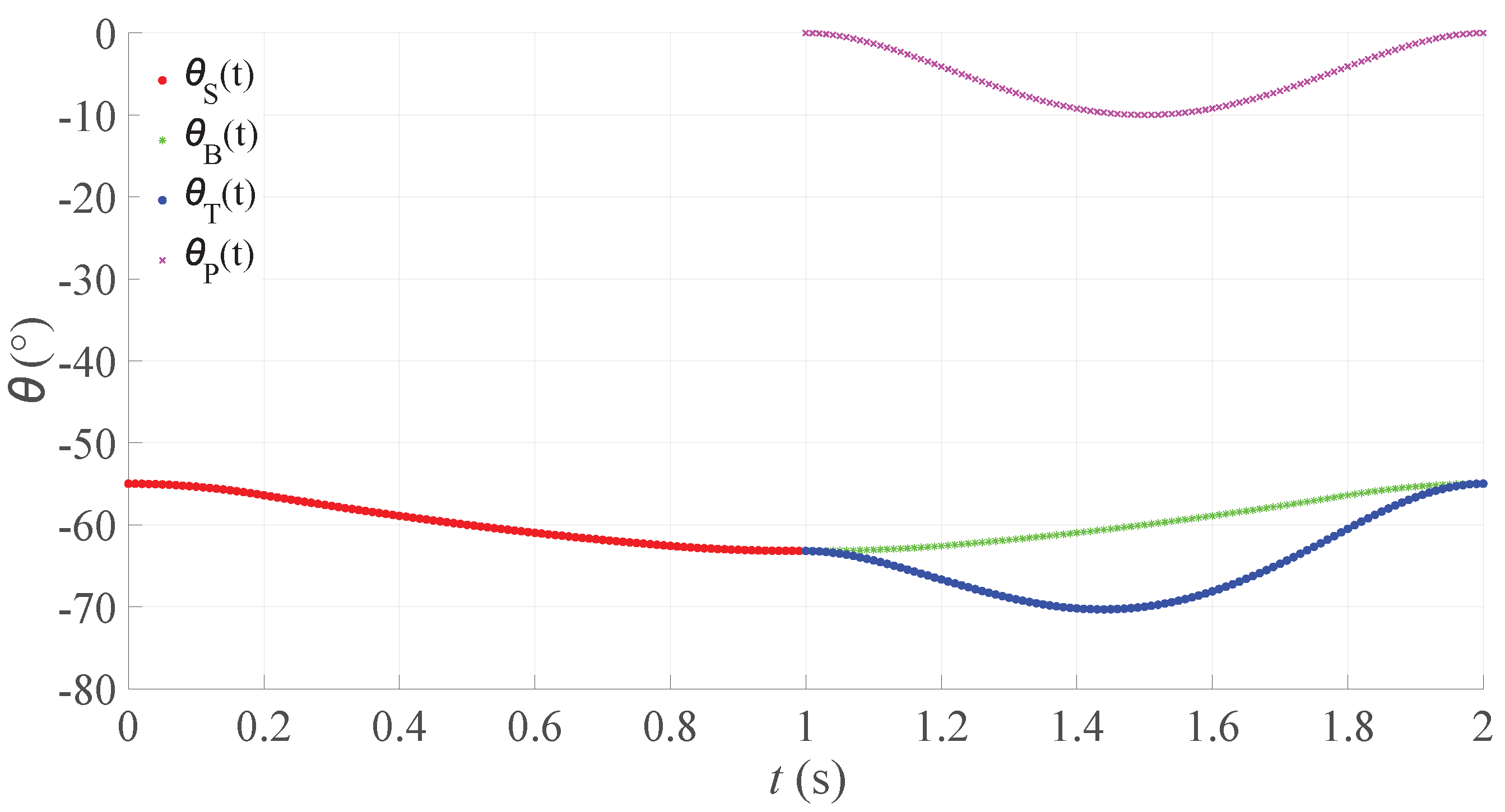
By combining ${\theta }_{\mathrm{S}}$(t) in support phase and ${\theta }_{\mathrm{T}}$(t) in transfer phase together, the total trajectory of one joint during a movement period in joint-space is defined as the dotted line in Figure 7. The red dotted line is ${\theta }_{\mathrm{S}}$(t). The blue dotted line is ${\theta }_{\mathrm{T}}$(t), and it is the superposition of the green line ${\theta }_{\mathrm{B}}\left(t\right)$ and the pink line ${\theta }_{\mathrm{P}}\left(t\right)$.

4.3. Verification of the Three-Element Trajectory Determination Method

The trajectory of one foot based on the three-element trajectory determination method during one movement period in Cartesian space is simulated in Figure 8, in which counter clockwise is selected as the positive direction and $T_b=0.2$, $T_f=1$.

From Figure 8a, it can be observed that, during the time $t\in (0,T_f)$, the foot’s coordinates in X and Z axes remain unchanged, and the robot only moves along the Y axis, which confirms that the robot is moving in a straight line. Figure 8b is the foot’s trajectory in space, the straight line is the trajectory in support phase, and the arc line is the trajectory in transfer phase.

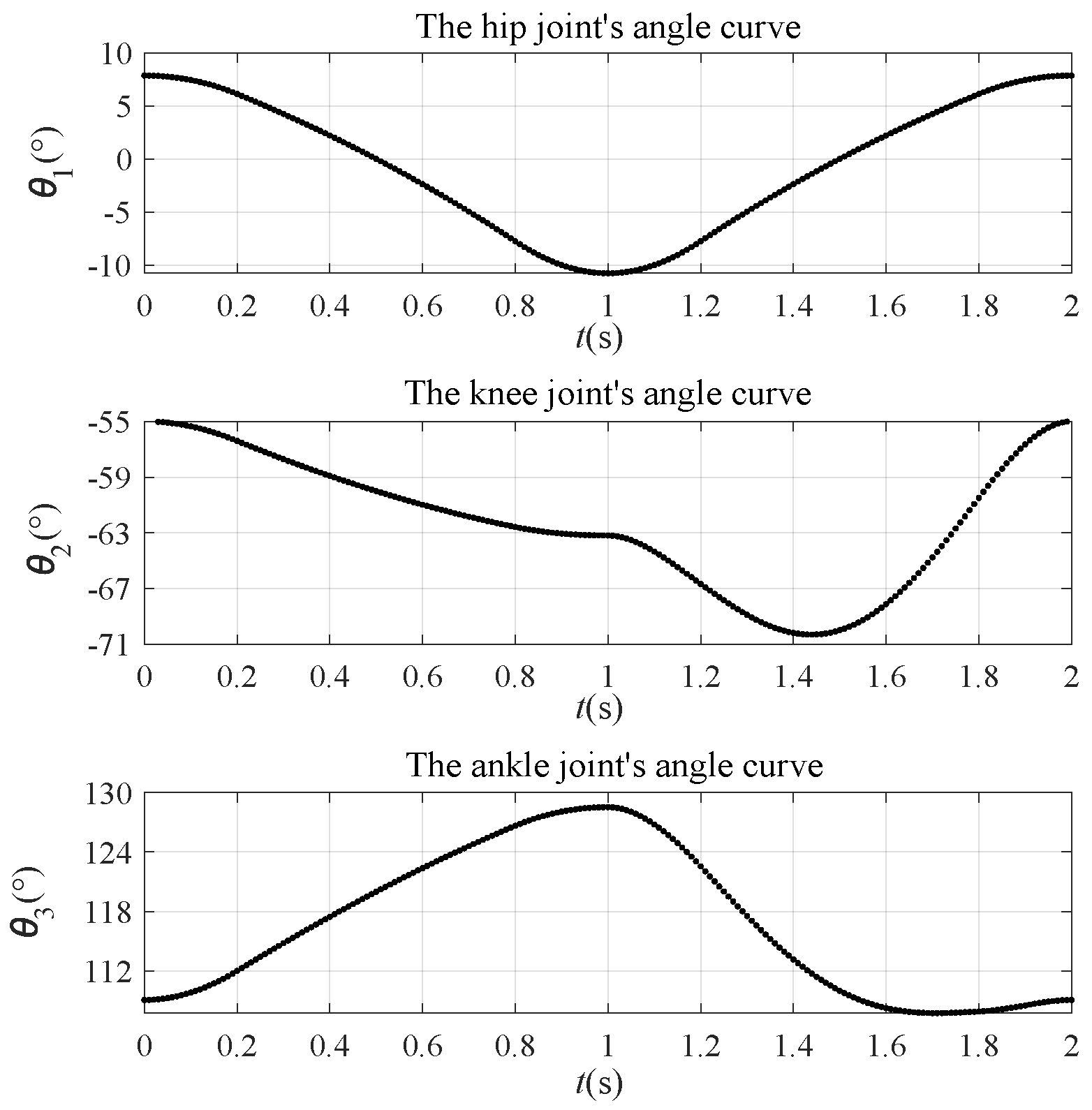
Here, we also provide the angle curve of the three joints as in Figure 9. We can observe that, while moving, all of the three angle curves are continuous and smooth, which further demonstrates the stability and practicability of our trajectory planning method for legged robots.

5. The Three-Element Trajectory Determination Method in Triangle Gait

The advantage of our designed trajectory method is reflected in the realization that the robot’s horizontal posture is maintained during movements. For the three elements, $\Delta \theta$ is set according to the feedback information from the foot. What else needs to be performed is to select the start point $P_0$ and the end point $P_1$. 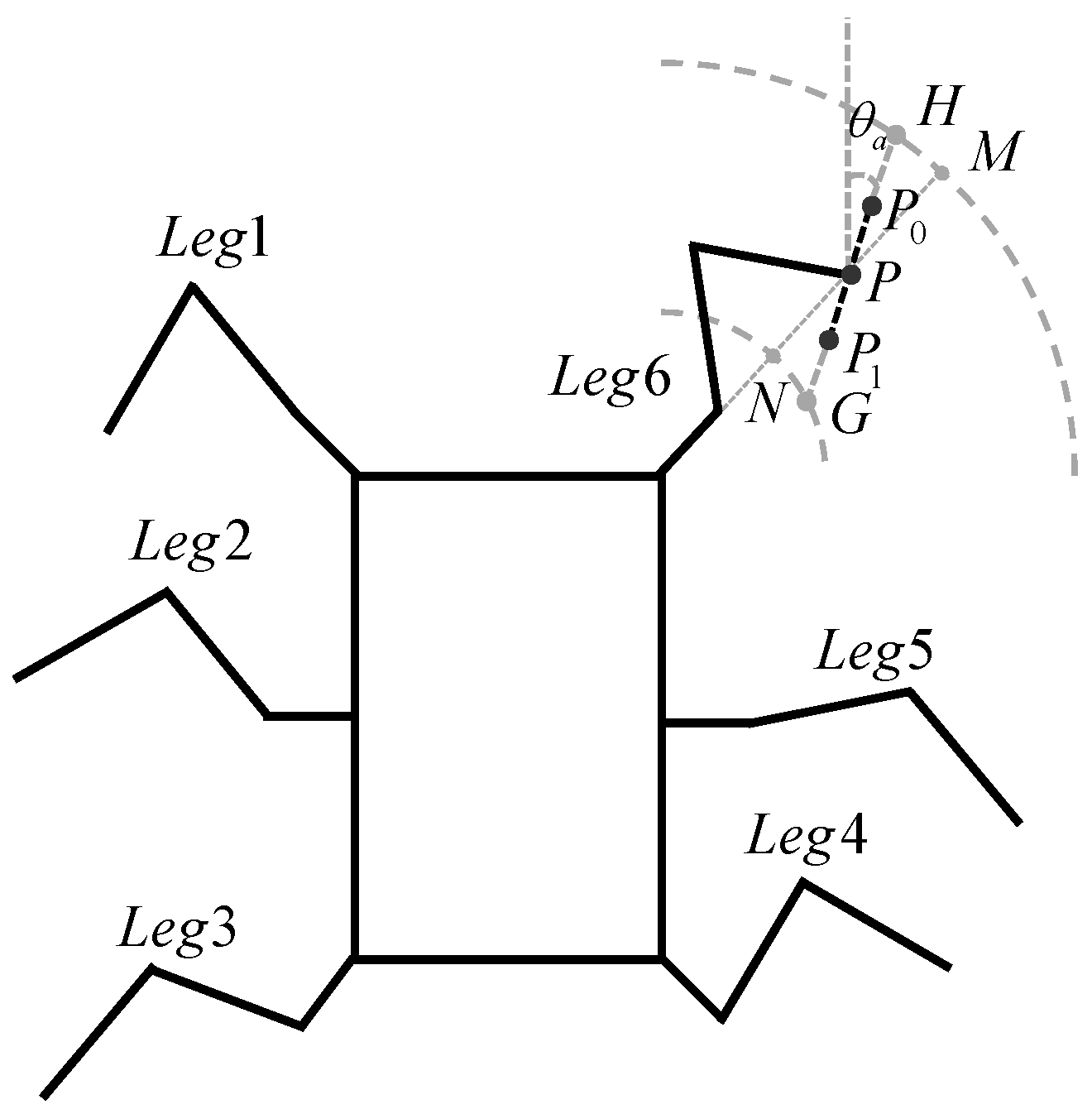Supposing the target height of the robot’s body is Z , target moving direction is ${\theta }_a$, and the moving step is D, then it can be divided into three steps for our method. The details are described by combining Figure 10.

5.1. Stable Point Determination

First of all, to improve our method’s stability and flexibility in triangle gait, in this paper, we treat the stable posture for a legged robot as the posture where $lin{k}_{i3}$ in Figure 1b is perpendicular to the ground and the hip joint’s angle ${\theta }_1$ in Figure 5 is simultaneously zero. The foot’s point is now called a stable point. As in Figure 10, the points on the line $\overline{MN}$ are all stable points. As $lin{k}_{i3}$ is perpendicular to the ground, by geometric knowledge, we obtain the following.

$${\theta }_3={\theta }_2+\frac{\pi }{3}.$$

(23)

For the foot’s inverse kinematics in (11), with the above conditions, there will be only one degree of freedom. To help the hexapod robot adapt to rugged terrains, we set Z as input so that we can obtain the expected stable point P.

5.2. Start Point and End Point Selection

After the stable point P is determined, what also needs to be performed is to select the start point $P_{\mathrm{s}}$ and the end point $P_{\mathrm{e}}$ of the support phase. For a hexapod robot, it is symmetric, and the triangle gait is simultaneously repetitive. Thus, the stable point during movement will be the middle point of the trajectory in the support phase. Supposing that the target moving direction is ${\theta }_a$, the trajectory in the support phase is along the line $\overline{P_0{P}_1}$, as shown in Figure 10. Ideally, $|P{P}_0|=|P{P}_1|=\frac{D}{2}$, and the coordinates of $P_0$ and $P_1$ can be computed. In reality, the feet can only reach a limited range (as in Figure 10, the foot of $Leg6$ can only arrive at the points between the two dotted arc lines); thus, the selection of $P_{\mathrm{s}}$ and $P_{\mathrm{e}}$ should depend on specific conditions.

Extend $P{P}_0$ and intersect it with the outer arc at point H. Extend $P{P}_1$ and intersect it with the inner arc at point G. If $min\{\left|PH\right|,\left|PG\right|\}\ge \frac{D}{2}$, this means both of the points $P_0$ and $P_1$ can be reached, and they can be the selected points. Then, the priority is given to movement stability, and all feet move equidistant around their respective stable points. If $\left|PH\right|\ge \frac{D}{2},\left|PG\right|<\frac{D}{2}$, this means the point $P_1$ cannot be reached, and the selected points are $P_0$ and G. If $\left|PH\right|<\frac{D}{2},\left|PG\right|\ge \frac{D}{2}$, this means the point $P_0$ cannot be reached, then the selected points are H and $P_1$. If $max\{\left|PH\right|,\left|PG\right|\}<\frac{D}{2}$, then the trajectory will be the line $\overline{HG}$. Thus, we have the following.

$$\left\{\begin{array}{c}\mathrm{If}min\{\left|PH\right|,\left|PG\right|\}\ge \frac{D}{2},P_{\mathrm{s}}=P_0\mathrm{and}{P}_{\mathrm{e}}=P_1,\\ \mathrm{If}\left|PH\right|\ge \frac{D}{2},\left|PG\right|<\frac{D}{2},P_{\mathrm{s}}=P_0\mathrm{and}{P}_{\mathrm{e}}=G,\\ \mathrm{If}\left|PH\right|<\frac{D}{2},\left|PG\right|\ge \frac{D}{2},P_{\mathrm{s}}=H\mathrm{and}{P}_{\mathrm{e}}=P_1,\\ \mathrm{If}max\{\left|PH\right|,\left|PG\right|\}<\frac{D}{2},P_{\mathrm{s}}=H\mathrm{and}{P}_{\mathrm{e}}=G.\end{array}\right.$$

(24)

Transform the start point $(x_{P_{\mathrm{s}}},y_{P_{\mathrm{s}}},z_{P_{\mathrm{s}}})$ and the end point $(x_{P_{\mathrm{e}}},y_{P_{\mathrm{e}}},z_{P_{\mathrm{e}}})$ that were obtained above under the world coordinate to the coordinate $\left\{O_{i0}\right\}$. Then, the trajectory of each foot can be planned by using the method in Section IV.

6. Experiment on Physical Robot in Real Environment

6.1. Triangle Gait Designed in Practice

Traditionally, the movement of a foot can be divided into support phase in $(0,T_f)$ and transfer phase in $(T_f,2T_f)$. For the triangle gait [24], when the feet of group A move as the support phase, the feet of group B move as the transfer phase and vice versa. In this paper, to better apply our trajectory method for legged robots in complex environments, we added an adjustment phase (AP) at the end of transfer phase so that the robot can adjust its foot position for trajectory planning in the next period to guarantee the accuracy of the movement. The triangle gait then, in practice, is designed as in Figure 11. For different terrains, the time for the adjustment phase $\Delta t_i$ can be different. However, when the feet of one group is in the adjustment phase, the feet of the other group will still be in the support phase in order to leave the following planning process unaffected.

6.2. Movement Control Flowchart

The movement control flowchart based on the above triangle gait is shown in Figure 12. For any leg, the follow situations may happen. When the leg is in the support phase, judging whether this phase has been completed needs to be performed. If not, keep moving along the planned trajectory; if it is performed, this means that the leg is ready for phase changing. When the foot is not in the support phase but already on the ground, this means that the foot touches the ground or obstacles in advance; here, the foot needs to replan its trajectory based on the ground’s height information, which is sensed by the designed foot sensing structure. When the foot is not on the ground, one situation is that the leg is in the transfer phase, then the foot moves along the planned trajectory. The other situation is that the leg has already finished the transfer phase but has not touched the ground, this situation happens when the ground’s height is lower than planned. Then, a new height $Z=Z+\Delta Z$ is set, and the foot needs to perform new trajectory planning in the adjustment phase based on Z information. When all legs are ready for phase changing, the phase is changed, and the robot keeps moving.

6.3. Experimental Results and Analysis

To prove the effectiveness of our method in complex environment, we situate the robot in two different real scenes.

6.3.1. Slope Experiment

The first scene that we chose is a slope outside with the angle of $7^{\circ }$. In Figure 13a–c, take $Foot5$ as an example; its trajectory planning is given as the red curve. This curve is similar to the simulated trajectory in Figure 8b except that the heights of the start point and the end point in support phase are not the same. At $t=12$ s, the $Foot5$ is on the ground, and it is ready for the transfer phase. At $t=13$ s, we can observe that $Foot5$ arrives at the top of the planned trajectory. At $t=14$ s, it falls to the ground and enters to the next support phase. This is a typical trajectory planning process. Figure 13d–f show the gait mode. In Figure 13f, at time $t=27$ s, the $Leg2$, $Leg4$, and $Leg6$ are in the air (transfer phase), while the other three legs are on the ground (support phase). At time $t=34$ s, as in Figure 13e, the phases are switched, the $Leg1$, $Leg3$, and $Leg5$ are in the transfer phase, and the $Leg2$, $Leg4$, and $Leg6$ are in support phase. The situation in Figure 13f is the same as the one in Figure 13d.

During the robot’s slope climbing, we mark its posture with a yellow line. What is worth pointing out is that, during all the movement, the robot can always keep its body horizontal, which is proof of the stability of our method.

Although this experiment is performed on a slope with the angle of $7^{\circ }$, after conducting a lot of tests, it is proved that the robot can adapt to a slope with any angle as long as the friction is sufficient.

6.3.2. Obstacle Experiment

To further show the robot’s strong movement ability, we situate the robot in an obstacle environment, as shown in Figure 14, where two obstacles with different height are placed inside. The robot’s movement is shown as in Figure 14. For the sake of description, we divide $Leg1$, $Leg3$, and $Leg5$ as the A group and $Leg2$, $Leg4$, and $Leg6$ as the B group.

In Figure 14a–c, we can observe that the A group is in the transfer phase. The $Leg1$ lifts up at the time $t=10$ s and touches the obstacle at time $t=12$ s. As the ground’s height information changes, there is an adjustment process for $Leg1$ as stated in the control flowchart in Figure 12. From Figure 14d on, the A group is in support phase, and the B group is in the transfer phase. This process finishes in Figure 14f at time $t=15$ s. In Figure 14g,h, the $Leg1$ moves on the top of obstacle 1. In Figure 14i, $Leg1$ starts to walk down the obstacle. Here, the foot tries to sense where the ground is based on the designed foot sensing structure in Figure 2. At the time $t=34$ s, the $Leg1$ touches the ground, and landing information is fed back. Figure 14l–p show the process of leaping over obstacle 2. In Figure 14p, all legs and feet are marked to help better understand the robot’s movement.

In this experiment, we also mark the robot’s posture. Results show that, although in a very complex environment, the robot with our trajectory planning method can still maintain horizontal posture.

7. Conclusions

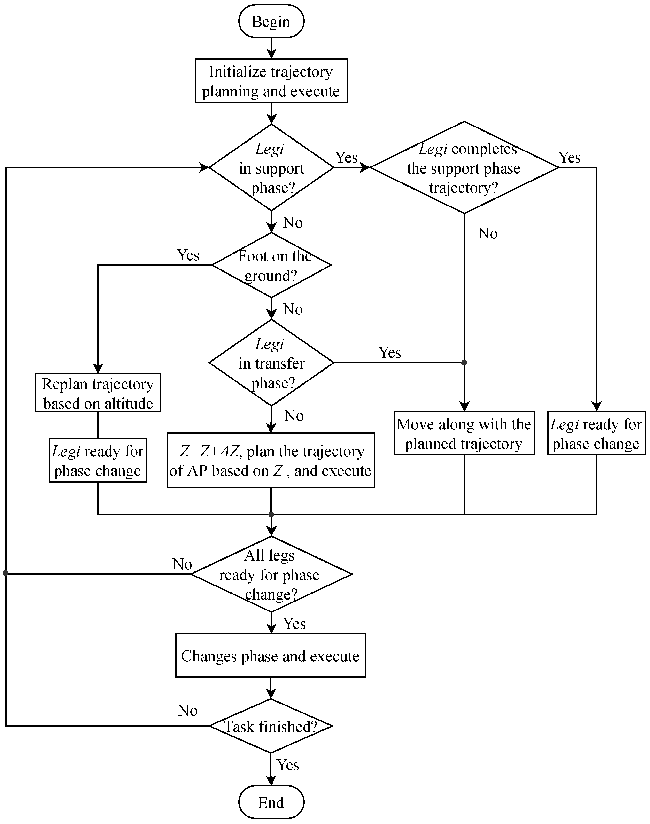
Legged robots have high movement flexibility, which makes them more suitable for various complex terrains. However, the complex control algorithm and trajectory planning also accompany the robot. Reasonable trajectory planning methods will greatly reduce the difficulty of control algorithm designs. Thus, this paper designs a new trajectory planning method for legged robots named the three-element trajectory determination method. Meanwhile, to realize this method’s application on a physical robot, this paper creates a new design of the legged robot’s foot sensing structure in order to help obtain landing information. To show how the method works, the details of its application in a triangle gait are given. Indicated by the observation of our experiments, this paper makes an improvement of the traditional triangle gait, where an adjustment phase is added at the end of transfer phase to help the robot adjust its foot position when it deviates from the original planned trajectory because of changing terrain. A control flowchart with the introduced adjustment phase is also given. Experiments are carried out in a slope environment and an obstacle environment. The results prove that our method is effective and stable in practice .

Hexapod robots have extensive prospect and are worth studying. In this paper, the improvement of the movement of hexapod robots mainly focuses on the trajectory planning method. In the future, we plan to take attitude information into account in order to develop novel control algorithm designs.