Article

Practical Formation Control for Multiple Anonymous Robots System with Unknown Nonlinear Disturbances

1
Marine Engineering College, Dalian Maritime University, Dalian 116026, China
2
College of Artificial Intelligence, Nankai University, Tianjin 300350, China
3
College of Engineering, Peking University, Beijing 100871, China
*
Author to whom correspondence should be addressed.
Appl. Sci. 2021, 11(19), 9170; https://doi.org/10.3390/app11199170
Submission received: 17 August 2021 / Revised: 26 September 2021 / Accepted: 30 September 2021 / Published: 2 October 2021
(This article belongs to the Section Robotics and Automation)

Abstract

:
This paper mainly investigates formation control problems for a group of anonymous mobile robots with unknown nonlinear disturbances on a plane, in which all robots can asymptotically converge to any formation patterns without collision, and maintain any required relative distance with neighboring robots. To solve this problem, all robots are modeled as kinematic points and can only acquire information from other robots and their targets. Furthermore, a flexible distributed control law is designed to solve the formation problem while no collisions between any robots can be guaranteed during the whole process. The outstanding feature of the proposed control method is that it can force all mobile robots to form not only uniform circle formations but also non-uniform and non-circular formations with moving target centers. At last, both theoretical analysis and numerical simulations show the feasibility of the proposed control law.

1. Introduction

In the last few years, owing to the rapid development in the field of networked control, technology for multiple mobile robots has developed, with various applications including specific tasks, e.g., environmental monitoring, surveillance, search and rescue, and exploration [1,2,3,4,5,6,7,8]. In such cooperative tasks and missions, it is beneficial to make all the robots move in a predetermined formation pattern in order to complete the assignments effectively and even to guarantee the performance of each related system, such as the robustness of group movement due to uncertain environmental disturbance. The great challenge for such pattern-forming problems of a group of robots lies in no individual being in charge of the central command. In other words, each robot can only use local information to implement the distributed control algorithms. Furthermore, the robots are physically distributed in many practical applications of multiple mobile robots in a wide range of areas.
In the field of multiple robot control, one of the hottest research topics is formation control, which involves guiding multiple mobile robots to form and maintain a predetermined geometric formation [9,10,11,12,13,14]. Specifically, the circular formation problem is among the most active topics of interest among researchers from various disciplines of science and engineering related to multiple mobile robots with close ties to formation control. The theoretical framework of circle formations for multiple mobile robots was introduced in [15,16,17,18], which was built on the earlier work of [19,20,21,22]. From then on, in the research community of systems and control, constant research efforts have been conducted on the developments of circular formation problem for multiple mobile robots, where the dynamics of robots are modeled as a single integrator [23], double integrators [24,25], nonlinear bifurcation dynamics [26], and even unicycles [27,28,29]. At the same time, some possible constrained scenarios are investigated involving time-delayed [27], locomotion constraints of robots [30,31,32], collision/deadlock avoidance [33,34,35], finite-time control [36,37], and input saturation [23].
According to the aforementioned existing literature, most of the results focused on equidistant circular formation control problems in the aspects of theory and application. However, when performing specific tasks, even distribution may not be the best configuration [38], forming arbitrary formations on a circle or plane has been studied by only a few recent works [25,30,36]. Wang et al. [36] designed distributed control protocols to control multiple robots to form a predetermined circular formation. In order to make the strategies more practical, the sampled data control protocol and finite-time control protocol were further extended. Wang et al. [30] handled the situation where the mobile robots are subject to motion constraints. To facilitate the establishment of a more general formative framework, Wang et al. [25] studied the general formation control problem of multiple mobile robots on a plane, where the robots are expected to maintain a distribution formation, and rotate or remain stationary around a stationary or moving target.
This paper aims to design a distributed control law that can ensure that multiple anonymous mobile robots form any non-uniform and non-circular formation with a moving target center on a plane. When the prescribed formation is set as an even distribution case, the non-uniform and non-circular formation thus reduces to the uniform circle formation. More specifically, the whole control objective can be divided into two sub-objectives. The first sub-objective is target circling, which indicates that all mobile robots must converge into a circular formation on a preset target as its center and rotate around the target with the same speed. At the same time, the second sub-objective is spacing adjustment, which means that all robots need to keep a desired distance from their neighboring robots without the requirement that all required distances between adjacent robots are the same. A networked system composed of multiple mobile robots under the models described by kinematic points is considered. Additionally, all robots move on a plane. Meanwhile, the robots are oblivious, anonymous, and unable to directly exchange information with each other. In other words, they can only perceive state information (including the relative position and relative speed) between the robot and its neighbors and the counterpart between the robot and the target.
This study focuses on keeping order and avoiding collisions between anonymous mobile robots, which makes the strategy more attractive when applying to real robot systems. More specifically, a system composed of multiple mobile robots, modeled as kinematic points and moves on the plane, is considered. The robots can only perceive the relative position and speed of neighboring robots and that between robots and the target. The difference between this paper and Ref. [39] is listed as follows. (1) Different from Ref. [39], which only pays attention to circle formation, the main goal of this paper is to design a general formation control protocol with obstacle avoidance conditions. (2) From a practical perspective, the proposed control protocol considers the case of unknown nonlinear disturbance, which makes it easy to use in real robot systems. The main contributions are summarized as follows: firstly, we design a distributed control law to deal with the formation problem asymptotically using the information of relative position and speed. Secondly, we divide the formation control problem into the control of the radial distance between robots and the target and the angle control between two robots and the target, in which the radial control and circumferential control do not affect each other. Especially in the case of moving targets, all mobile robots are required to track moving targets while maintaining the desired distances between neighboring robots. At last, both theoretical analysis and numerical simulations are provided to demonstrate the effectiveness of the proposed control laws.
The remainder of the paper is organized as follows. In Section 2, the basic notation is introduced and the formation control problem is formulated. A flexible distributed control law is proposed as well as the stability analysis based on it for the concerned systems is provided in Section 3. Numerical experimental results illustrating the application of our proposed control protocol are in Section 4. In Section 5, we conclude and suggest some possible further research topics.

2. Preliminaries and Problem Formulation

In this section, we first give the notation used throughout the paper and then formulate the formation control problem for multi-robots systems.

2.1. Preliminaries

Let R , R > 0 , R 0 , and N stand for sets of real numbers, positive real numbers, non-negative real numbers, and natural numbers, respectively. R m × n denotes a m × n real matrix. For matrix A, A represents its Euclidean norm, A denotes its -norm and A T denotes its transpose.

2.2. Problem Formulation

Consider N, N 2 , mobile robots, labeled as p 1 , p 2 , , p N and a free moving target labeled c to be around on an obstacle-free plane, as shown in Figure 1. All robots are initially located on the plane randomly and no two robots are collinear with the moving center point c. From the standpoint of the system analysis, the position of each robot p i , i 1 , 2 , , N , denoted by [ x i , y i ] , i 1 , 2 , , N in a prior Cartesian coordinates system. Without loss of generality, all the robots is tagged counterclockwise by p 1 , p 2 , , p N around target c, as shown in Figure 1.
Let G = ( V , E ) be the neighboring relationships among robots in the system, where V = { 1 , 2 , , N } is a set of robots, E = { ( 1 , 2 ) , ( 2 , 3 ) , , ( N 1 , N ) , ( N , 1 ) } stands for a set edges. That is, each robot has only two adjacent neighboring robots, which are in front or behind it. The set of two neighbors of the robot p i can be denoted by N i = { i , i + } , where
i + = i + 1 when i = 1 , 2 , , N 1 , 1 when i = N ,
and
i = N when i = 1 , i 1 when i = 2 , 3 , , N .
Define r i ( t ) = [ x i ( t ) , y i ( t ) ] T R 2 as the position of the robot p i , and r c ( t ) = [ x c ( t ) , y c ( t ) ] T R 2 denotes the positions of target c on the plane, at time t. Then, each robot p i ’s model, similar to [39], can be described as
r ˙ i ( t ) = u i ( t ) + g i ( x i ( t ) , t ) , i = 1 , 2 , , N ,
where u i R 2 is the control input of the robot p i and g i ( x i ( t ) , t ) denotes uncertain disturbances. Note that there exists a non-negative and known constant ω , such that the uncertain disturbances term g i ( x i ( t ) , t ) satisfies | g i ( x i ( t ) , t ) | ω < ( k r + 1 ) ( r ˜ i ( t ) R i ) , where k r , r ˜ i ( t ) and R i is the parameter which will be introduced later.
For the convenience of mathematical expression, let
r ˜ i ( t ) = r i ( t ) r c ( t ) , i = 1 , 2 , , N ,
be the relative position between the robot p i and the target c, which is measured by the robot p i at time t. The relative velocity between the robot p i and the target c measured by robot p i is presented as
v ˜ i ( t ) = r ˜ ˙ i ( t ) = v i ( t ) v c ( t ) , i = 1 , 2 , , N .
where v c ( t ) denotes the center point position.
Similarly, the relative position between the robot p i and its neighbor p i + measured by the robot p i at time t is described as
r ˜ i + ( t ) = r i + ( t ) r i ( t ) , i = 1 , 2 , , N .
The relative velocity between the robot p i and its neighboring robot p i + measured by the robot p i at time t is expressed as
v ˜ i + ( t ) = r ˜ ˙ i + ( t ) = v i + ( t ) v i ( t ) , i = 1 , 2 , , N .
Using a similar derivation process as before, it follows that r ˜ i + ( t ) , v ˜ i ( t ) represent the relative position, and the relative velocity between the robot p i and the robot p i , respectively.
Furthermore, a clear description of the variables α i + is given as the angle distance from the robot p i to the robot p i + , which can be calculated by rotating the ray c p i counterclockwise, extending from the target c to the robot p i until reaching the robot p i + . Similarly, α i is the angle distance from the robot p i to the robot p i . It is worthy to point out that the angle distance is defined to be positive if the ray c p i is rotated in the counterclockwise direction relative to the ray c p i + .
Similarly, referring to Equations (4)–(7), the definitions of the robot p i relative to its neighboring robot p i are written as
r ˜ i ( t ) = r ˜ i ( t ) , ( i V ) , v ˜ i ( t ) = v ˜ i ( t ) , ( i V ) , r ˜ ( t ) = [ r ˜ 1 ( t ) , r ˜ 2 ( t ) , , r ˜ n ( t ) ] , α ˜ ( t ) = [ α 1 + ( t ) , α 2 + ( t ) , , α n + ( t ) ] .
Considering that the initial states of all tagged N anonymous robots can be represented mathematically and the possible practical applications of the proposed control law for the multiple robot systems, two necessary properties of the N-robot system are given as below [38,39].
Definition 1
(Order preservation). Given a multi-robot system on a plane, which is composed of N mobile robots, the spatial ordering of robots is preserved according to control laws u i ( t ) , i = 1 , 2 , , N , if N robots are initially arranged in a counterclockwise order. For all t > 0 , the solution to the system (3) can guarantee N robots remain in the original order.
Definition 2
(Collision avoidance). Given a multi-robot system, it consists of N mobile robots on a plane. If N robots are initially arranged in a counterclockwise order on the plane, all the robots have the collision avoidance characteristics. For any two robots i, j ( i j ) , for all t > 0 , the solution of the system (3) satisfies r i r j > 0 .
We can obtain that the order preservation condition is sufficient but not necessary for the collision avoidance condition.
Given two N-dimensional vectors
α * = [ α 1 * , α 2 * , , α N * ] , ( i V , α i * > 0 , i V α i * = 2 π )
and
R * = [ R 1 , R 2 , , R N ] , ( i V , R i > 0 )
Suppose that each robot p i can only get the original information of related variables with respect to r ˜ i ( t ) , v ˜ i ( t ) , r ˜ i + ( t ) , v ˜ i + ( t ) , r ˜ i ( t ) , v ˜ i ( t ) , and then a parameter vector which can be presented in a synthesis form
X ˜ i ( t ) = [ r ˜ i ( t ) , v ˜ i ( t ) , r ˜ i + ( t ) , v ˜ i + ( t ) , r ˜ i ( t ) , v ˜ i ( t ) ] .
Then, a flexible distributed protocol is proposed as
u i ( t ) = F ( X ˜ i ) , i { 1 , 2 , , N } .
Moreover, a concerned formation problem on the plane is formulated as follows.
Definition 3
(Formation problem on a plane). For any admissible formations that can be characterized by α * and R * , the distributed control protocol u i = F ( X ˜ i ) , i = 1 , 2 , , N is designed, so that under any initial conditions, when N robots are arranged counterclockwise on a plane, the system’s solution converges to the equilibrium point r * satisfies (11). Namely, all mobile robots globally approach their desired locations asymptotically to form a desired formation.
a ) lim t + r ˜ ( t ) = R * b ) lim t + α ˜ ( t ) = α *

3. Distributed Hybrid Formation Control

3.1. Distributed Control Law Design

According to X ˜ i , the following information can be calculated, including α i + , α i , α ˙ i + , α ˙ i , the angular velocity ω i of robot p i relative to c (counterclockwise is positive), the velocity v i ( t ) of target c, r ˜ ˙ i ( t ) , the unit vector e r of r ˜ i ( t ) , and e θ ( e θ = e z × e r ). Further, we have
X i = X ˜ i { α i , α i + , α ˙ i , α ˙ i + , ω i , v c ( t ) , e r , e θ }
Therefore, a general control law is designed as
u i ( t ) = F ( X i ) = v c ( t ) + v i θ ( t ) + v i * ( t ) + g i ( x i ( t ) , t )
where v i θ ( t ) and v i * ( t ) denote the circumferential control and the radial control function for the robot p i , respectively.
The circumferential control v i θ ( t ) is essentially related to the distance from the robot p i to the center point c. One simple form of this function can be represented as
v i θ ( t ) = ω i * ( X i ) r ˜ i ( t ) e θ
The radial control function v i * ( t ) is considered such that it equals to exchange information whenever any robots get contact with robot p i
v ˙ i * ( t ) = α i * ( X i ) = ( α r * ( X i ) r ˜ i ( t ) ω i + r ˜ i ( t ) ω i ω i * ( X i ) ) e r + ( α θ * ( X i ) r ˜ i ( t ) + ω i * ( X i ) r ˜ ˙ i ( t ) ) e θ
where ω i * ( X i ) , α r * ( X i ) and α θ * ( X i ) are three independent variables without specific forms.

3.2. Stability Analysis

Theorem 1.
Assuming the control for robot p i presented in (12) has appropriate tuning functions v i θ ( t ) and v i * ( t ) , the control objective can be reached.
Proof. 
For any robot p i ( i V ) , the relative position r ˜ i ( t ) satisfies
r ˜ ˙ i ( t ) = v ˜ i ( t ) = v i ( t ) v c ( t )
Then,
r ˜ ¨ i ( t ) = v ˙ i ( t ) v ˙ c ( t ) = v ˙ i θ ( t ) + v ˙ i * ( t ) = ( ω i * ( X i ) r ˜ i ( t ) e θ ) · + α i * ( X i )
Together with d d t e θ = ω i e r , it yields
r ˜ ¨ i ( t ) = ω ˙ i * ( X i ) r ˜ i ( t ) e θ + ω i * ( X i ) r ˜ ˙ i ( t ) e θ ω i ω i * ( X i ) r ˜ i ( t ) e r + ( α r * ( X i ) r ˜ i ( t ) ω i + r ˜ i ( t ) ω i ω i * ( X i ) ) e r + ( α θ * ( X i ) r ˜ i ( t ) + ω i * ( X i ) r ˜ ˙ i ( t ) e θ = ( α r * ( X i ) r ˜ i ( t ) ω i ) e r + ( ω ˙ i * ( X i ) r ˜ i ( t ) + α θ * ( X i ) r ˜ i ( t ) + 2 ω i r ˜ ˙ i ( t ) ) e θ
Besides, r ˜ ˙ i ( t ) can also be rewritten as
r ˜ ˙ i ( t ) = r ˜ ˙ i ( t ) e r + r ˜ i ( t ) ω i e θ
Consequently,
r ˜ ¨ i ( t ) = ( r ˜ ¨ i ( t ) r ˜ i ( t ) ω i 2 ) e r + ( ω ˙ i r ˜ i ( t ) + 2 ω i r ˜ ˙ i ( t ) e θ
By combining (13) and (14), we get
α r * ( X i ) r ˜ i ( t ) ω i = r ˜ ¨ i ( t ) r ˜ i ( t ) ω i 2 ( ω ˙ i * ( X i ) r ˜ i ( t ) + α θ * ( X i ) r ˜ i ( t ) + 2 ω i r ˜ ˙ i ( t ) = ω i r ˜ i ( t ) + 2 ω i r ˜ ˙ i ( t )
which is simplified as
r ˜ ¨ i ( t ) = α r * ( X i ) + r ˜ i ( t ) ( ω i 2 ω i ) ω ˙ i = ω ˙ i * ( X i ) + α θ * ( X i )
That is to say, under the designed control law, we can separate the control of ω i from r ˜ i ( t ) . Equation (15) indicates that the control of ω i only relates to ω i * ( X i ) and α θ * ( X i ) , meanwhile the control of r ˜ i ( t ) only relates to α r * ( X i ) . Namely, the formation control problem is decomposed into the radial control and the circumferential control.
However, Equation (15) does not satisfy with the anti-collision condition and the convergence condition. Thus, specific forms of ω i * ( X i ) , α r * ( X i ) , and α θ * ( X i ) are given to meet both convergence condition the anti-collision condition.
(1)
Example of α r * ( X i )
α r * ( X i ) has the form as
α r * ( X i ) = k r ( r ˜ i ( t ) R i ) 2 k r r ˜ ˙ i ( t )
where k r > 0 .
When the initial condition fulfills i V and r ˜ ˙ i ( 0 ) > k r r ˜ i ( 0 ) , the movement of all robots satisfies the convergence condition and the anti-collision condition. According to
r ˜ ¨ i ( t ) = α r * ( X i )
We get
r ˜ ¨ i ( t ) = k r ( r ˜ i ( t ) R i ) 2 k r r ˜ ˙ i ( t )
As a critically damped motion differential equation, its solution is written as
r ˜ i ( t ) = R i + ( ( r ˜ i ( 0 ) R i ) + ( r ˜ ˙ i ( 0 ) + ( r ˜ i ( 0 ) R i ) k r ) ) e k r t
Seeking the limit of Equation (17), we get
lim t + r ˜ i ( t ) = R i
meets the convergence condition (11).
The first derivative of r ˜ i ( t ) is
r ˜ ˙ i ( t ) = k r ( r ˜ ˙ i ( 0 ) + ( r ˜ i ( 0 ) R i ) k r ) t + r ˜ ˙ i ( 0 )
When
t 1 = r ˜ ˙ i ( 0 ) ( r ˜ ˙ i ( 0 ) + ( r ˜ i ( 0 ) R i ) k r ) ) k r > 0
At t 1 , r ˜ ˙ i ( t 1 ) = 0 , r ˜ i ( t ) reaches its extreme value.
To sum up, if the initial conditions satisfy
i V , r ˜ i ( 0 ) > 0 , r ˜ ˙ i ( 0 ) > k r r ˜ i ( 0 )
Then,
i V , t > 0 , r ˜ i ( t ) > 0
A Lyapunov function candidate is considered as
V ( r ˜ i ( t ) ) = ( R i r ˜ i ( t ) ) 2 .
Then, the derivative of V ( r ˜ i ( t ) ) along the trajectories leads to
V ˙ ( r ˜ i ( t ) ) = 2 ( R i r ˜ i ( t ) ) r ˜ ˙ i ( t ) = 2 ( r ˜ i ( t ) R i ) a r * 2 k r k r 2 ( r ˜ i ( t ) R i ) + g i ( x i ( t ) , t ) = k r ( r ˜ i ( t ) R i ) 2 + a r * ( r ˜ i ( t ) R i ) k r + 2 ( r ˜ i ( t ) R i ) g i ( x i ( t ) , t ) 2 k r ( r ˜ i ( t ) R i ) 2 2 ( r ˜ i ( t ) R i ) 2 + 2 ω ( r ˜ i ( t ) R i ) ( 2 k r + 2 ) ( r ˜ i ( t ) R i ) 2 + 2 ω ( r ˜ i ( t ) R i )
where k r > 0 . From ω < ( k r + 1 ) ( r ˜ i ( t ) R i ) , (21) can be rewritten as
V ˙ ( r ˜ i ( t ) ) 0 .
It can be further proven that r ˜ i ( t ) = R i is the maximum invariant set in { r ˜ i ( t ) M 1 | V ˙ ( r ˜ i ( t ) ) = 0 } . Additionally, each solution starting in r ˜ i ( t ) M 1 approaches to r ˜ i ( t ) = R i as t obtained from LaSalle s theorem in [40]. Thus, we conclude that if the initial condition meets the condition show as Equation (19), r ˜ i ( t ) satisfies the anti-collision (2) and convergence condition (11) under the designed α r * ( X i ) .
(2)
Example of ω i * ( X i ) and α θ * ( X i )
Define
Δ α i = α i * α i + α i * α i α i * + α i *
Then,
Δ α ˙ i = α i * α ˙ i + α i * α ˙ i α i * + α i *
ω i * ( X i ) and α θ * ( X i ) are rearranged as
ω i * ( X i ) = α i * α ˙ i + α i * α ˙ i α i * + α i * = Δ α ˙ i α θ * ( X i ) = k θ Δ α i + 2 k θ Δ α ˙ i
where k θ > 0 .
We only consider the initial condition satisfies
i j , ω i = ω j
According to
ω ˙ i = ω ˙ i * + α θ *
We get
ω i = ω i * + τ = 0 t α θ * d τ + C θ
Based on the initial condition, we can obtain i V , α ˙ i + = 0 , further Δ α ˙ i = 0 . Thus, at t = 0 , there exists ω ˙ i = ω ˙ i * such that C θ = 0 gives. Therefore,
ω ˙ i = ω ˙ i * + τ = 0 t α θ * d τ
Take the derivation of (26), we have a critically damped vibration equation for Δ α i
Δ α ¨ i = ω ˙ i * = α θ * = k θ Δ α i 2 k θ Δ α ˙ i
Taking the initial condition Δ α ˙ i = 0 into consideration, the solution to (27) is
Δ α i ( t ) = Δ α i 0 ( 1 + k θ t ) e k θ t
where Δ α i 0 = Δ α i ( 0 ) .
For convenience, define
f ( t ) = ( 1 + k θ t ) e k θ t
Further, we get
f ( 0 ) = 1 f ˙ ( t ) = k θ t e k θ t t > 0 , 0 < f ( t ) < 1 lim t + f ( t ) = 0
Substituting Equation (23) into Equation (28), we have
α i * α ˙ i + α i * α ˙ i = ( α i * + α i * ) Δ α i 0 f ( t )
Based on Equation (8), we obtain
α n * 0 0 0 α 1 * α 2 * α 1 * 0 0 0 0 α 3 * α 2 * 0 0 0 0 0 α n * α n 1 * α ˜ = α 1 * + α n * α 2 * + α 1 * α 3 * + α 2 * α n * + α n 1 *
A general solution of (30) is expressed as
α ˜ ( t ) = x ( t ) α * + ( α ˜ ( 0 ) α * ) f ( t )
Summing up each column vector of Equation (31), we have
i = 1 n α i + ( t ) = x ( t ) i = 1 n α i * + ( i = 1 n α i + ( 0 ) i = 1 n α i * ) f ( t )
According to i = 1 n α i + ( t ) = 2 π and i = 1 n α i * ( t ) = 2 π , we have
2 π = 2 π x ( t ) , x ( t ) = 1 .
The solution of (30) is
α ˜ ( t ) = α * + ( α ˜ ( 0 ) α * ) f ( t )
Written in a component form as
α ˜ i ( t ) = α i * + ( α ˜ i ( 0 ) α i * ) f ( t )
which is rewritten as
α i + ( t ) = α i * ( 1 f ( t ) ) + α ˜ i + ( 0 ) f ( t )
According to Equation (29), we get
lim t + α i + ( t ) = α i *
satisfying the convergence condition, where α i * > 0 , α i + ( t ) > 0 .
When t > 0 , from Equation (29), we get f ( t ) > 0 , 1 f ( t ) > 0 . Thus,
t > 0 , α i + ( t ) > 0
satisfies the anti-collision condition.
To sum up, we give the form of ω i * ( X i ) , α i * ( X i ) , α θ * ( X i ) as in Equations (16) and (24), and prove that the motions of multiple mobile robots satisfy the anti-collision (2) and the convergence condition (11).

4. Numerical Examples

In this section, for the designed examples of ω i * ( X i ) , α r * ( X i ) and α θ * ( X i ) , simulation results are given. The initial condition is set as t = 0 , i V , v c = v i , and k r = k θ = 1 .

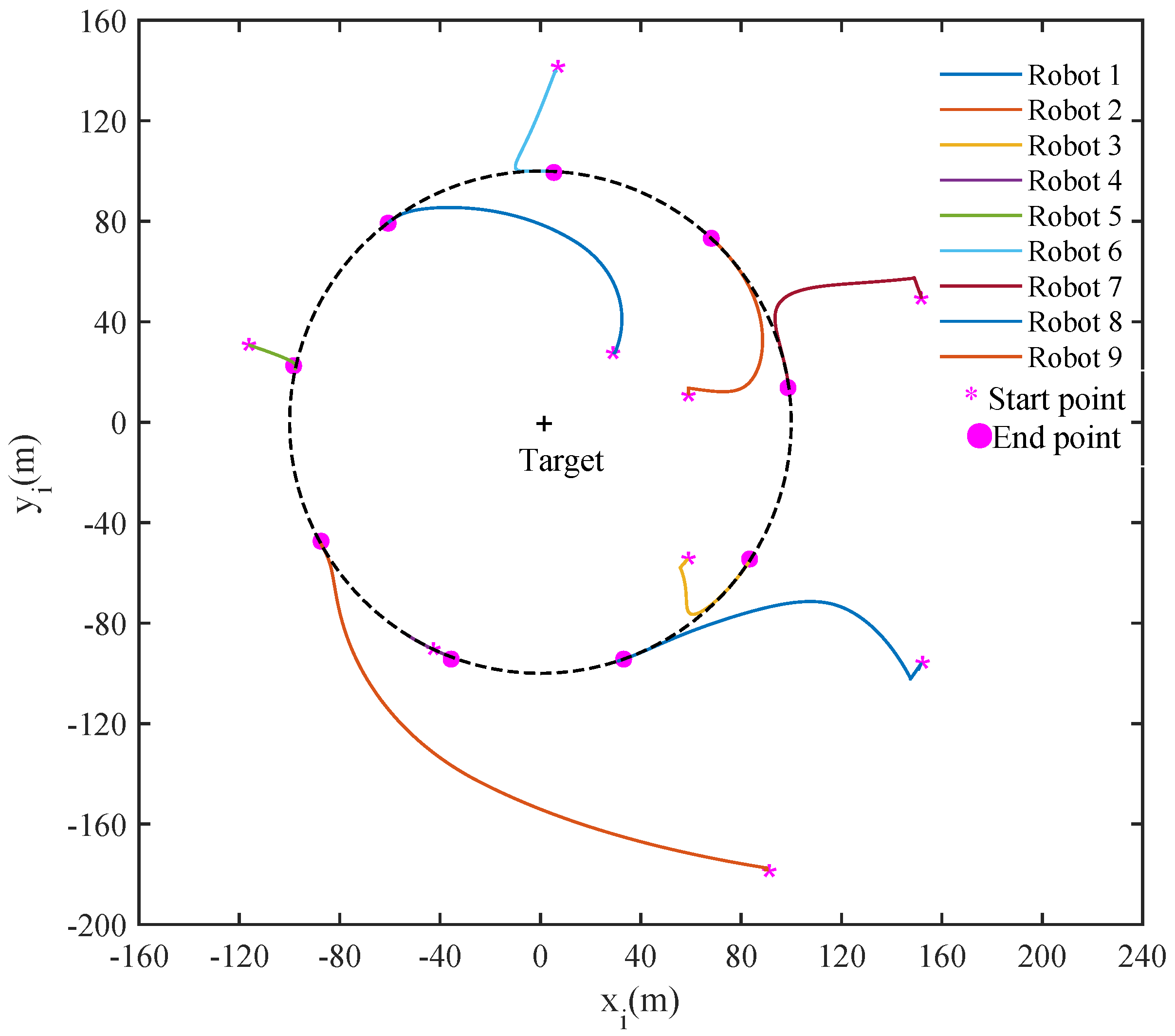
4.1. Uniform Circle Formation

As shown in Figure 2, considering a multiple mobile robots system, consists of nine robots, we set the center of the circular formation at (0, 0) m on the plane. The radius of the desired enclosing uniform circular formation is set as R i = 100 m , i = 1 , 2 , . . 9 . The initial positions of robots are generated randomly.
The simulation results are shown in Figure 3 and Figure 4. From Figure 3, we can observe that the group of mobile robots move asymptotically to the pink dots so as to form the prescribed uniform circle under the designed control law (12). As shown in Figure 4, the evolution of the difference between the current position and the required counterpart between each pair of adjacent robots shows that the desired uniform circle formation can be achieved asymptotically. We conclude that using the proposed control law, the multi-robot system has the characteristics of order preservation and collision avoidance.

4.2. Non-Uniform and Non-Circular Formation

This simulation considers a multi-robot system composed of nine robots and the center point position (0, 0) m with the velocity (0, 0) m/s. The initial positions of the nine robots are generated randomly. At the same time, the predetermined distribution formation is derived from archimedean spiral antennas, as shown in Figure 5.
The simulation results are shown in Figure 6 and Figure 7. As shown in Figure 6, the simulation results indicate that the group of mobile robots move asymptotically to target points so as to form the prescribed non-uniform and non-circular formation under the proposed control law (12). We can observe from Figure 7, the system has the characteristics of order preservation and collision free under the proposed control law.

5. Conclusions

This paper studied the formation control problem for multiple anonymous mobile robots on a plane. To solve this problem, we first designed a distributed control law, which can guide all the robots to converge to a uniform circle with a prescribed center and a non-uniform and non-circular formation with a moving target center. Then, we proved that the proposed control law could solve the formation control problem asymptotically and ensure that there is no collision between robots. At last, we show that theoretically, the research results provide an effective method for solving the problem of formation control for multiple robots systems, which is supplementary to the existing results. Since certain parameters in the proposed controller have precise physical meanings related to the rotation of the agent around the target, they can be set more reasonably and efficiently in practical applications. Moreover, each robot can merely perceive the relative positions from its limited neighbors and the target. Using the information from sensors, controllers can transmit action orders to robots for formation tasks.

Author Contributions

P.X. and J.T. conceived and designed the research; P.X. designed and performed the simulation experiment; G.X. and M.X. contributed to the theory studies. All authors have read and agreed to the published version of the manuscript.

Funding

This research was funded by the National Key Research and Development Project (Grant No. 2019YFC1510900) and the National Natural Science Foundation of China (Grant Nos.61973172, 61973175, 62003175).

Institutional Review Board Statement

Not applicable.

Informed Consent Statement

Not applicable.

Data Availability Statement

The data used to support the findings of this study are available from the corresponding author upon request.

Acknowledgments

This work was supported by the National Key Research and Development Project (Grant No. 2019YFC1510900) and the National Natural Science Foundation of China (Grant Nos.61973172, 61973175, 62003175).

Conflicts of Interest

The authors declare no conflict of interest.

References

  1. Han, Q.; Liu, P.; Zhang, H.; Cai, Z. A wireless sensor network for monitoring environmental quality in the manufacturing industry. IEEE Access 2019, 7, 78108–78119. [Google Scholar] [CrossRef]
  2. Mas, I.; Kitts, C.A. Dynamic control of mobile multirobot systems: The cluster space formulation. IEEE Access 2014, 2, 558–570. [Google Scholar] [CrossRef]
  3. Napora, S.; Paley, D.A. Observer-based feedback control for stabilization of collective motion. IEEE Trans. Control Syst. Technol. 2013, 21, 1846–1857. [Google Scholar] [CrossRef] [Green Version]
  4. Chung, T.H.; Hollinger, G.A.; Isler, V. Search and pursuit-evasion in mobile robotics: A survey. Auton. Robots 2011, 31, 299–316. [Google Scholar] [CrossRef] [Green Version]
  5. Ren, W. Collective motion from consensus with cartesian coordinate coupling. IEEE Trans. Autom. Control 2009, 54, 1330–1335. [Google Scholar] [CrossRef]
  6. Ding, W.; Yan, G.; Lin, Z. Pursuit formations with dynamic control gains. Int. J. Robust Nonlin 2012, 22, 300–317. [Google Scholar] [CrossRef]
  7. Bullo, F.; Cortes, J.; Martinez, S. Distributed Control of Robotic Networks; Princeton University Press: Princeton, NJ, USA, 2009. [Google Scholar]
  8. Pavone, M.; Arsie, A.; Frazzoli, E.; Bullo, F. Distributed algorithms for environment partitioning in mobile robotic networks. IEEE Trans. Autom. Control 2011, 56, 1834–1848. [Google Scholar] [CrossRef]
  9. Yu, W.W.; Zheng, W.Z.; Chen, G.R.; Lv, J.H. Distributed control gains design for consensus in multi-agent systems with second-order nonlinear dynamics. Automatica 2013, 49, 2107–2115. [Google Scholar] [CrossRef]
  10. Zhao, Y.; Duan, Z.S.; Wen, G.H.; Zhang, Y.J. Distributed finite-time tracking control for multi-agent systems: An observer-based approach. Syst. Control Lett. 2013, 62, 22–28. [Google Scholar] [CrossRef]
  11. Xu, P.; Zhao, H.F.; Xie, G.M.; Tao, J.; Xu, M.Y. Pull-based distributed event-triggered circle formation control for multi-agent systems with directed topologies. Appl. Sci. 2019, 9, 4995. [Google Scholar] [CrossRef] [Green Version]
  12. Marcolino, L.S.; Jiang, A.X.; Tambe, M. Multi-agent team formation: Diversity beats strength? In Proceedings of the 23th International Conference Artificial Intelligence (IJCAI ’13), Beijing, China, 3–9 August 2013; pp. 279–285. [Google Scholar]
  13. Pinto, T.; Morais, H.; Oliveira, P.; Vale, Z.; Praça, I.; Ramos, C. A new approach for multi-agent coalition formation and management in the scope of electricity markets. Energy 2011, 36, 5004–5015. [Google Scholar] [CrossRef] [Green Version]
  14. Chen, C.L.P.; Yu, D.; Liu, L. Automatic leader-follower persistent formation control for autonomous surface vehicles. IEEE Access 2019, 7, 12146–12155. [Google Scholar] [CrossRef]
  15. Défago, X.; Souissi, S. Non-uniform circle formation algorithm for oblivious mobile robots with convergence toward uniformity. Theor. Comput. Sci. 2008, 396, 97–112. [Google Scholar] [CrossRef]
  16. Flocchini, P.; Prencipe, G.; Santoro, N. Self-deployment of mobile sensors on a ring. Theor. Comput. Sci. 2008, 402, 67–80. [Google Scholar] [CrossRef] [Green Version]
  17. Guo, J.; Yan, G.F.; Lin, Z.Y. Local control strategy for moving-target-enclosing under dynamically changing network topology. Syst. Control Lett. 2010, 59, 654–661. [Google Scholar] [CrossRef]
  18. Xiao, Y.; Liu, L. Distributed circular formation control of ring-networked nonholonomic vehicles. Automatica 2016, 68, 92–99. [Google Scholar]
  19. Défago, X.; Konagaya, A. Circle formation for oblivious anonymous mobile robots with no common sense of orientation. In Proceedings of the Second ACM International Workshop on Principles of Mobile Computing, Toulouse, France, 30–31 October 2002; pp. 97–104. [Google Scholar]
  20. Marshall, J.; Broucke, M.; Francis, B. Formations of vehicles in cyclic pursuit. IEEE Trans. Autom. Control 2004, 49, 1963–1974. [Google Scholar] [CrossRef]
  21. Cheng, S.; Liu, L.; Xu, S.Y. Circle formation control of mobile agents with limited interaction range. IEEE Trans. Autom. Control 2018, 64, 2115–2121. [Google Scholar]
  22. Chatzigiannakis, I.; Markou, M.; Nikoletseas, S. Distributed circle formation for anonymous oblivious robots. In Proceedings of the International Workshop on Experimental and Efficient Algorithms, Angra dos Reis, Brazil, 25–28 May 2004; pp. 159–174. [Google Scholar]
  23. Song, C.; Liu, L.; Feng, G. Coverage control for mobile sensor networks with input saturation. Unmanned Syst. 2016, 4, 15–21. [Google Scholar] [CrossRef]
  24. Shi, Y.; Li, R.; Teo, K. Cooperative enclosing control for multiple moving targets by a group of agents. Int. J. Control 2015, 88, 80–89. [Google Scholar] [CrossRef]
  25. Wang, C.; Xia, W.; Xie, G. Limit-cycle-based design of formation control for mobile agents. IEEE Trans. Autom. Control 2019, 65, 3530–3543. [Google Scholar] [CrossRef]
  26. Chen, H.; Sun, J.; Li, K.; Wang, M. Autonomous spacecraft swarm formation planning using artificial field based on nonlinear bifurcation dynamics. In Proceedings of the AIAA Guidance, Navigation, and Control Conference, AIAA2017-1269, Grapevine, TX, USA, 9–13 January 2017. [Google Scholar]
  27. Brinón-Arranz, L.; Seuret, A.; Canudas-de-Wit, C. Cooperative control design for time-varying formations of multi-agent systems. IEEE Trans. Autom. Control 2014, 59, 2283–2288. [Google Scholar] [CrossRef] [Green Version]
  28. Zheng, R.; Liu, Y.; Sun, D. Enclosing a target by nonholonomic mobile robots with bearing-only measurements. Automatica 2015, 53, 400–407. [Google Scholar] [CrossRef]
  29. Yu, X.; Liu, L. Cooperative control for moving-target circular formation of nonholonomic vehicles. IEEE Trans. Autom. Control 2016, 62, 3448–3454. [Google Scholar] [CrossRef]
  30. Wang, C.; Xie, G.; Cao, M. Controlling anonymous mobile agents with unidirectional locomotion to form formations on a circle. Automatica 2014, 50, 1100–1108. [Google Scholar] [CrossRef]
  31. Peng, L.; Ren, W.; Song, Y.D. Distributed multi-agent optimization subject to nonidentical constraints and communication delays. Automatica 2016, 65, 120–131. [Google Scholar]
  32. Leonard, N.E.; Paley, D.A.; Davis, R.E.; Fratantoni, D.M.; Lekien, F.; Zhang, F.M. Coordinated control of an underwater glider fleet in an adaptive ocean sampling field experiment in Monterey Bay. J. Field Robot. 2010, 27, 718–740. [Google Scholar] [CrossRef]
  33. Damasceno, B.C.; Xie, X. Deadlock-free scheduling of manufacturing systems using Petri nets and dynamic programming. IFAC Proc. Vol. 1999, 32, 4870–4875. [Google Scholar] [CrossRef]
  34. Sherif, F.; Balakrishnan, S.; ElMekkawy, T. Deadlock prevention and performance oriented supervision in flexible manufacturing cells: A hierarchical approach. Robot. Comput. Integr. Manuf. 2011, 27, 591–603. [Google Scholar]
  35. Mehdi, F.; Gunawan, I.; Smith-Miles, K. Resolution of deadlocks in a robotic cell scheduling problem with post-process inspection system: Avoidance and recovery scenarios. In Proceedings of the 2015 IEEE International Conference on Industrial Engineering and Engineering Management (IEEM), Singapore, 6–9 December 2015. [Google Scholar]
  36. Wang, C.; Xie, G.; Cao, M. Forming circle formations of anonymous mobile agents with order preservation. IEEE Trans. Autom. Control 2013, 58, 3248–3254. [Google Scholar] [CrossRef]
  37. Liu, R.; Cao, X.; Liu, M. Finite-time synchronization control of spacecraft formation with network-induced communication delay. IEEE Access 2017, 5, 27242–27253. [Google Scholar] [CrossRef]
  38. Song, C.; Liu, L.; Feng, G.; Xu, S.Y. Coverage control for heterogeneous mobile sensor networks on a circle. Automatica 2016, 63, 349–358. [Google Scholar] [CrossRef]
  39. Wang, C.; Xie, G. Limit-cycle-based decoupled design of circle formation control with collision avoidance for anonymous agents in a plane. IEEE Trans. Autom. Control 2017, 62, 6560–6567. [Google Scholar] [CrossRef]
  40. Mao, X. Stochastic versions of the LaSalle theorem. J. Differ. Equ. 1999, 153, 175–195. [Google Scholar] [CrossRef] [Green Version]
Figure 1. Formation of N robots on a plane. (a) Robots initially locate on a plane. (b) Robots form a predetermined formation around the target.
Applsci 11 09170 g001
Figure 2. Desired uniform circle on a plane.
Applsci 11 09170 g002
Figure 3. Trajectories of nine robots on the plane at t ( 0 , 10 ] when k r = 1 and k θ = 1 .
Applsci 11 09170 g003
Figure 4. Simulation results of the uniform circle formation when k r = 1 and k θ = 1 : (a) Evolution of r i ( t ) r c for i = 1 , 2 , , N on the plane at t ( 0 , 10 ] . (b) Evolution of α + α * for i = 1 , 2 , , N on the plane at t ( 0 , 10 ] .
Applsci 11 09170 g004
Figure 5. Desired non-uniform and non-circular formation on a plane.
Applsci 11 09170 g005
Figure 6. Trajectories of nine robots on the plane at t ( 0 , 10 ] when k r = 1 and k θ = 1 .
Applsci 11 09170 g006
Figure 7. Simulation results of the non-uniform and non-circular formation when k r = 1 and k θ = 1 : (a) Evolution of r i ( t ) r c for i = 1 , 2 , , N on the plane at t ( 0 , 10 ] . (b) Evolution of α + α * for i = 1 , 2 , , N on the plane at t ( 0 , 10 ] .
Applsci 11 09170 g007
Publisher’s Note: MDPI stays neutral with regard to jurisdictional claims in published maps and institutional affiliations.

