Abstract
Brain responses are often studied under strictly experimental conditions in which electroencephalograms (EEGs) are recorded to reflect reactions to short and repetitive stimuli. However, in real life, aural stimuli are continuously mixed and cannot be found isolated, such as when listening to music. In this audio context, the acoustic features in music related to brightness, loudness, noise, and spectral flux, among others, change continuously; thus, significant values of these features can occur nearly simultaneously. Such situations are expected to give rise to increased brain reaction with respect to a case in which they would appear in isolation. In order to assert this, EEG signals recorded while listening to a tango piece were considered. The focus was on the amplitude and time of the negative deflation (N100) and positive deflation (P200) after the stimuli, which was defined on the basis of the selected music feature saliences, in order to perform a statistical analysis intended to test the initial hypothesis. Differences in brain reactions can be identified depending on the concurrence (or not) of such significant values of different features, proving that coterminous increments in several qualities of music influence and modulate the strength of brain responses.
1. Introduction
Conventional studies on the brain’s perception and processing of music using electromagnetic approaches—for example, magnetoencephalography (MEG) and electroencephalography (EEG)—focus on recognizing the neural processing of non-natural sounds that are chosen for their adaptation to the requirements of each specific test. This wide scope of research on music and the brain incorporates pure vs. complex tones as stimuli [1,2], as well as consonant vs. dissonant sequences [3,4], chordal cadences [5], and simple monophonic melodies, some of them accompanied by harmony, while others are not [6,7].
However, studying continuous listening and its effects on brain response from the naturalistic paradigm perspective together with the presence of coterminous musical features is still an important issue to be analyzed. This research involves natural music listening [8] and, thus, the subjects’ perception of the distinctive properties of music—impurity, spontaneity, expectancy, interaction, etc.—together with their link to musical analysis for the identification of relevant coterminous features in order to reveal the integration of the brain’s response to auditory features [9] in naturalistic music listening.
In this context, Pearce et al. [10] found that in comparison with high-probability notes, low-probability ones prompted a greater late negative event-related potential (ERP) factor, raising the beta-band oscillation over the parietal lobe. The component was elicited at an interval of 400–450 ms. A study of the awareness of musical resonance by selecting instrumental sounds as stimuli was carried out by Meyer et al. [11]. They highlighted how instruments with different resonances stimulated regions of the brain that were correlated with auditory and emotional imagery tasks apart from enhanced N1/P2 responses.
In addition, a number of functional MRI (fMRI) research works have examined the use of natural and continuous music and the consequences of a sudden change in some features. This was done in spite of the fact that hemodynamic reactions that are registered with fMRI are slow, which obscures quick feature alterations that happen at key points of musical pieces. In this context, extracts from real musical pieces have generally been observed [12,13], and more recently, complete pieces [14,15] have been considered. In addition, Alluri et al. [16] investigated the neural processing of specific musical properties using fMRI by listening to an orchestral music recording, associating fMRI data with computational musical features. In [17], using diverse pieces of music, musical features were correlated with activation in a variety of brain areas. Nevertheless, it must be taken into account that brain activity, when studied using fMRI, is averaged across a few seconds because the subtleties of hemodynamic reactions registered with fMRI are slow in contrast with the methods of electromagnetic brain studies.
In this work, we created an innovative experimental paradigm for analyzing brain responses to music by automatically extracting a number of key musical features from full pieces of music and checking their concurrent incidence individually, by pairs, or in groups of three simultaneous features. Often, research on the effects of concurrent or synchronized stimuli on the brain response focuses on the presence of stimuli of a diverse nature, and the audio–visual scenario is the most widely examined [18,19,20,21], though occasionally, solely the audio context is considered with respect to concurrent sounds [9,22]. However, our hypothesis and purpose are different from previous ones: We aim to investigate whether electrophysiological brain responses change when musical features extracted from a piece of music change concurrently. We opted to study electric brain activity provoked by the acoustic properties of Adios Nonino by Astor Piazzolla, which is the same Tango Nuevo piece that Alluri et al. studied using fMRI. Alluri et al. [16] found that low-level musical properties, such as those that we use, give rise to measured brain signals peaking in temporal regions of the scalp; as opposed to this, we consider EEG signals and, most importantly, coterminous features. Note that low-level audio features, such as the ones we use, can be considered those that can be extracted from short audio excerpts.
The existing understanding of artificial sound is applied in our research into continuous music. We assume that swift variations in real musical features will provoke similar sensory components, as shown by traditional ERP studies that examined tone stimuli. Further, we assume that ERP amplitudes will depend on the scale of the quick growth of individual feature values [23] and the length of the previous period of time with low feature values [24], as demonstrated by Poikonen [25], but we now treat ERP variations that are related to coterminous musical feature changes.
We will mostly observe signals at the positive sensory deflation taking place 200 milliseconds following the onset of the stimulus (P200) and the negative sensory deflation taking place 100 milliseconds after (N100). So, we perform comparisons regarding the brain’s reactions in relation to isolated/concurrent abrupt changes in the selected features. Note that the P1/N1/P2 responses were previously considered regarding the appearance of acoustical features in relation to their event rate [26]. In addition, it is often assumed that magnitudes in an acoustical feature are linearly related to ER amplitudes [26,27]. We consider a similar context, but one that is related to the timing of different acoustical features.
Our focus is on the time and frequency features—brightness, zero-crossing rate, and spectral flux (Section 2.4)—because we want to investigate quick neural responses in the auditory areas of the temporal cortices [16]. In addition, we consider the root mean square (RMS) feature, which is connected to loudness. We study all of these features in isolation, in pairs, or in groups of three, hypothesizing that the concurrent incidence of alterations of features will cause stronger reactions than isolated changes in the features. Feature conjunction is a main aspect of the analysis performed in this work, as opposed to the consideration of isolated musical feature saliences.
In the next section, the data employed and the processing stages of the EEG and audio signals will be described. Then, the results of the analysis of the signals and a discussion will be exposed. Finally, some conclusions will be drawn in Section 4.
2. Data and Methods
In this section, the data acquisition methodology, the stimulus, and the database employed are described, as well as the processing and data analysis schemes and the specific features and feature sets considered for the identification of the points of interest in the audio sample.
2.1. Subjects
The dataset employed came from the same dataset employed in [25], which has been used in other studies [26,28]. The data were used under a specific agreement. Briefly, our subset contained samples from eleven right-handed Finns with a near-even ratio of males to females. We chose the samples for our subset so that no artifacts close to the points of interest were observed. The average age of the subjects was , ranging from 20 to 46. None of the subjects reported previous neurological conditions or hearing loss.
There were no professional musicians among the participants, though some subjects reported a musical education and others reported an active interest in music (singing, dancing, learning to play an instrument, or making music on a computer). The experimental protocol under which the dataset was recorded was approved by the Committee on Ethics of the Faculty of the Behavioral Sciences of the University of Helsinki and was carried out in compliance with the Declaration of Helsinki.
2.2. Stimulus
The stimulus considered in the experiment was the Tango Nuevo piece “Adios Nonino” by Astor Piazzola [16]; it is an min piece recorded in a live concert in Lausanne, Switzerland. These are the same data and stimuli as those used in [17].
Note that Adios Nonino has a versatile musical structure and large variability, which makes it an interesting piece for finding variations in audio features, their concurrence, and their relation to EEG signals.
2.3. Technology Used and Procedure
The procedure followed is thoroughly described in [17]; here, a brief summary is exposed: The subjects were presented with the piece of music using the Presentation 14.0 program and Sony MDR-7506 headphones. The intensity was 50 dB above the individually set auditory threshold [17]. The researcher played the piece back after a brief discussion with the subjects via microphone. The subjects were asked to listen quietly to the music with their eyes open to maintain their attention toward the music; on the other hand, note that keeping their eyes closed could be problematic for our experiments, since this enhances the alpha rhythm, which can disturb the N1-/P2-evoked response measurements [26,29].
EEG data were recorded using BioSemi bioactive electrode caps with a 10–20 system [30], with five external electrodes placed at the left and right mastoids, on the tip of the nose, and around the right eye, both vertically and horizontally. A total of 64 EEG channels were sampled at 600 Hz.
2.4. Processing and Analyzing Data
Feature extraction was performed by using MIRtoolbox (version 1.7) [31]. MIRtoolbox is a set of MATLAB tools that extract various musical aspects in relation to sound engineering, psychoacoustics, and music theory. MIRtoolbox is designed to process audio files and can process a number of time and frequency features in audio. Brightness, RMS, zero-crossing rate, and spectral flux were the short-term low-level features chosen in this experiment. They were collected in a window of 25 ms with overlap, which is common in Music Information Retrieval (MIR) [32]. The audio signal was sampled at 44,100 Hz, so every frame was 2205 samples long: , with . With the exception of the RMS, these features coincided with the ones discovered to provoke auditory activation in the temporal cortices in the experiment by Alluri et al. [16]. The description of the features is given in the following:
- Brightness: Brightness is defined as the spectral energy above a certain frequency with respect to the total energy for each analysis window [31]. It can be measured as follows:where N is the number of samples of the discrete Fourier transform (DFT) of : , the signal in the analysis window, and k stands for the smallest frequency bin corresponding to a frequency larger than the cutoff frequency defined to measure brightness; this frequency was set to 1500 Hz in MIRtoolbox. Low values of brightness mean that a small percentage of the spectral energy is in the higher frequency range of the frequency spectrum, and vice versa.
- Root mean square (RMS): This feature is connected to a song’s dynamics or loudness. It is defined as the square root of the average of the squared amplitude samples:Lower sounds have lower RMS values [31].
- Zero-crossing rate: This rate is defined by the number of times the audio waveform crosses the zero level per unit of time [33]. It is an accepted indicator of noisiness: A lower zero-crossing rate indicates less noise in the considered audio frame [31]. It can be measured as follows:with for positive amplitudes and otherwise.
- Spectral flux: This feature comes from the Euclidean norm of the difference between the amplitude of consecutive spectral distributions [34]:where X and Y stand for the DFT of two consecutive audio frames: the current one, , and the previous window, , respectively. represents the Euclidean norm.The spectral flux value is high in the event of great variation in spectral distribution in two consecutive frames. The curves of spectral flux show peaks at the transition between successive chords or notes [31].
Now, recall that we are considering continuous music listening, so, in our research, the duration of low-level feature values before their swift growth is consistent with the inter-stimulus interval (ISI) of prior studies; there are no recurrent silent intervals in real music. In this paper, we call the ISI-like period the preceding low-feature phase (PLFP). We consider EEG signals linked to concurrent musical properties that are changing and, most specially, doing so concurrently. It is assumed that prolonged ISI enhances the early sensory ERP responses and that extended PLFP will lead to higher ERP amplitudes when listening to continuous music.
Thus, we define triggers for instants when some properties rise after long preceding low-feature phases (PLFPs) [24,25]. Thus, instants with a quick rise of a musical property are located. Specifically, we test different lengths of the PLFPs—from 200 to 1000 ms—and we set the speed of the growth of the feature to be higher than the magnitude of rapid increase (MoRI) [25], which we set to 75 ms. The moving averages in 75 ms windows of the song for each feature are determined, and the change in magnitude is defined on the basis of the moving average value. The range of the MoRI goes from to of the feature’s mean; with this, the triggers considered valid are the ones preceded by a PLFP under the lower mean value threshold.
With this, significant instants are identified using each of the features selected. In addition, instants at which certain combinations of features significantly change at the same time are selected. Thus, we consider features both individually and, specifically, jointly, which is our main objective.
2.5. EEG Signal Analysis
Again, MATLAB was used to pre-process the subjects’ EEG data. The electrode on the tip of their nose served as a reference [25]. The data were low-pass filtered at 70 Hz to retain EEG signal information from the beta and gamma bands. A notch filter was applied at 50 Hz to avoid interference from the power line, high-pass filtered at 1 Hz to avoid drifts [26]. This gave a continuous data stream with a length between 297,000 and 321,600 samples from the position of the trigger for the initial synchronization at the beginning to the end of the recording session.
Continuous EEG data were split into sets of intervals according to the triggers defined in the musical stimuli beginning 200 ms before the trigger and ending 700 ms after. We defined the baseline corresponding to the 500 ms time frame before the trigger. Intervals with amplitudes over V were eliminated to ensure eye artifact removal (following [35]), and all of the selected intervals underwent a visual inspection to ensure that no artifacts were present.
Then, in order to identify features or feature sets that affected, from a statistical point of view, the subjects’ EEG signals at the selected intervals, the N100 and P200 components were considered. The N100 component was sought in each combination of regions/features (see Section 2.6) to locate a minimum of the subjects’ average within a window ranging between 10 and 300 ms from the trigger. Similarly, the P200 component was sought by finding the maximum in an interval ranging from 200 to 500 ms.
We acquired the N100 and P200 amplitudes in relation to the changes in musical features or feature sets, which were considered to be the source of the ERP. We followed the same approach with their latency.
2.6. Data Computation and Naming Convention
The EEG samples were processed as described previously in this section by using the points of interest obtained by identifying instants at the audio frame level when two or more audio features stood out; we also did so individually. Specifically, the features and feature sets considered and the notation employed are shown in Table 1.

Table 1.
Features and feature sets under consideration and their notation.
Regarding the behavior of the selected features in the chosen piece of music, the following facts must be observed:
- There were not enough time points at which RMS and ZCR changed concurrently to perform an analysis.
- There was not an acceptable number of time points with three coterminous features changing simultaneously to study this phenomenon in each of the different combinations of variables by threes, so we considered these combinations as a whole.
- It was not possible to find points with the four features changing at the same time, so this scenario will not be considered.
Regarding the number of trials, the minimum accepted number of identified time points for the definition of trials for the analysis was 12. The analysis of EEG data was considered separately according to the regions. In each cortical region, the computed EEG signals were obtained as the average across all of the subjects and the electrodes corresponding to the area under analysis; specifically, the following areas were considered:
- Frontal: Average of Fz, F1, F2, F3, and F4.
- Central: Average of Cz, C1, C2, C3, and C4.
- Parietal: Average of Pz, P1, P2, P3, and P4.
- Occipital: Average of Oz, O1, O2, PO7, and PO8.
- Temporal: Average of T7, T9, TP7, and TP9. Note that only the left temporal side was studied.
For the sake of simplicity, not all of the cortical regions were evaluated. Only the two that presented more significant oscillations will be discussed; these are the occipital region and the temporal region. Recall that it was suggested by Alluri et al. [16] that resonance-related acoustic aspects of musical pieces played without interruption have a positive correlation with the activation of major temporal lobe regions.
3. Results and Discussion
In this section, the results found after processing the audio data for the identification of the points of interest and the EEG data (as previously described) are shown. Statistical analyses of the ERPs are performed.
To begin with the observation of the behavior of EEG data, in Figure 1, the EEG data acquired in response to abrupt changes in only brightness, only spectral flux, and jointly in Brightness and Spectral Flux are shown. Note that all of the figures are drawn using the same scale for easy comparison. The average signal is drawn, and its standard deviation is represented by the shade. The occipital and temporal regions seem to be where oscillations were more strongly marked. However, it can be observed that the amplitudes of the N100 and P200 components were larger when the brightness and spectral flux were concurrent. In addition, larger standard deviations of each peak are also appreciable in Figure 1c.
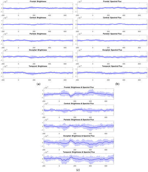
Figure 1.
(a) EEG data related to changes in brightness. (b) EEG data related to changes in spectral flux. (c) EEG data related to changes in both brightness and spectral flux.
These particularities can be exposed in a different manner by displaying the distribution of the peaks in box plots for both the amplitude and time of the events.
Figure 2 shows the different distributions of the amplitude and latency of N100 and P200 when an abrupt change in the musical piece was due to RMS evolution (Figure 2a); the same is shown for spectral flux (Figure 2b). The case of a significant and concurrent variation in both RMS and spectral flux is shown in Figure 2c. According to Figure 2, the P200 amplitudes in particular are wider when both the RMS and spectral flux present changes compared to when the RMS or spectral flux changes significantly but alone. This behavior is more remarkable in the temporal and occipital regions.
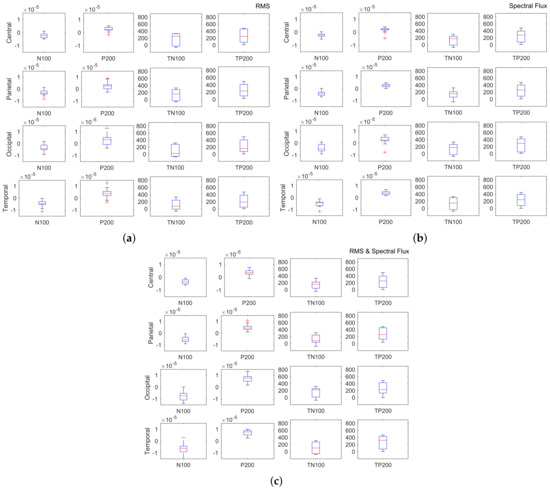
Figure 2.
(a) Box-plot distributions of the N100 and P200 amplitudes (N100, P200) and latencies (TN100, TP200) due to RMS changes. (b) Box-plot distributions of the N100 and P200 amplitudes (N100, P200) and latencies (TN100, TP200) due to spectral flux changes. (c) Box-plot distributions of the N100 and P200 amplitudes (N100, P200) and latencies (TN100, TP200) due to coterminous RMS and spectral flux changes.
Considering N100 and P200 by groups and cortical regions, it is possible to test if their distributions are different depending on the presence of significant changes in the feature or feature set under consideration. First, the Shapiro–Wilk test of normality was used to check that all of the EEG components were distributed normally. Then, multi-sample ANOVA was used to compare the different combinations that could reflect changes in the N100 and P200 amplitudes and latencies. For this purpose, a commonly accepted significance level of was chosen to reject the null hypothesis, . The results of this statistical analysis for assessing the existence of differences in the EEG signals in the different cases considered will be discussed next.
3.1. Analysis of the N100 Amplitude
Regarding the N100 amplitude, the ANOVA tests showed that the means of the following pairs in the occipital region were significantly different: x1–x7, x2–x7, x3–x5, x3–x7, and x4–x7; likewise, the following pairs in the temporal region were also significantly different: x1–x5, x1–x7, x1–x8, x2–x7, x3–x7, x4–x7, x6–x7, and x7–x9; the p-values are provided in Figure 3a and Figure 4a, respectively.
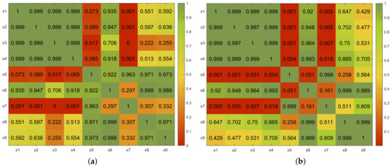
Figure 3.
Occipital region. Comparisons of p-values obtained with ANOVA by pairs. (a) N100 amplitude. (b) P200 amplitude.
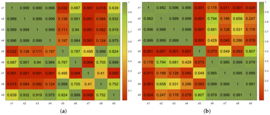
Figure 4.
Temporal region. Comparisons of p-values obtained with ANOVA by pairs. (a) N100 amplitude. (b) P200 amplitude.
It is remarkable that these differences were found between isolated features and combinations of two features regardless of the nature of the individual features and the presence of one of the single features in the pair of features under comparison. For example, the x7 feature set contained brightness (x1) and spectral flux (x4); nevertheless, significant differences in the N100 amplitude were found between x1–x7 and x4–x7, as well as between x2–x7 and x3–x7, which seems to indicate that it was the coincidence of the features that was responsible for the differences, and not their specific relations regarding their nature.
In addition, observe that differences were also found regarding the behavior with respect to single features and the x8 feature set, though their means were not considered statistically different by the test.
Surprisingly, in light of the previous observation, no statistically significant differences were found between the x6 feature set and the individual features of x1 to x4, though the p-values found were larger than in the set of comparisons between individual features (see Figure 3a and Figure 4a).
Finally, it is interesting to observe that low p-values were found regarding the comparisons of x6–x7 and x7–x8 in the temporal and occipital regions that were analyzed. Although the null hypothesis was not rejected in these cases, except in the case of the x6–x7 comparison in the temporal region (Figure 4a), the p-values found seem to suggest some differences in those comparisons, which could be due to the different natures of ZCR vs. spectral flux and brightness vs. RMS and their interpretation in the brain.
3.2. Analysis of the P200 Amplitude
Considering the P200 amplitude, an analysis similar to the one performed for the N100 amplitude was carried out. The results show the same trend as in the previous case. These results are shown graphically and numerically in the heat maps in Figure 3b and Figure 4b for the occipital and temporal regions, respectively.
The test of the hypothesis on the occipital P200 data revealed that the hypothesis was rejected in the following cases: x1–x5, x1–x7, x2–x5, x2–x7, x3–x5, x3–x7, x4–x5, and x4–x7. Observe the coincidences in these results between the x5 and x7 feature sets and the individual features. Furthermore, regarding the the temporal region, the null hypothesis was rejected in the following tests: x1–x5, x1–x7, x1–x9, x2–x5, x3–x5, x4–x5, and x4–x7.
These observations and their correlation with the results regarding the N100 amplitude highlight the relevance of the combination defined by the x5 and x7 feature sets to elicit brain activity versus the appearance of significant values of single features.
3.3. Overall Considerations of the N100 and P200 Amplitude Analysis
Overall, regarding the observed behavior of the N100 and P200 amplitudes in the regions considered, the sets of isolated features of x1, x2, x3, and x4 constituted a group in which the hypothesis test performed by pairs did not indicate the rejection of the null hypothesis in any case, which implies similar responses from the statistical point of view.
Likewise, the group formed by the x5 to x9 feature sets showed similar behavior, except in the case of the N100 amplitude in the temporal region for the feature sets x6–x7 and x7–x9. So, we can conclude that, in general, sets with two coincident features elicit similar responses from the point of view of the N100 and P200 amplitudes, as the x5 and x7 feature sets, which include brightness and RMS and brightness and spectral flux, respectively, are especially relevant.
The behavior of x9 was diverse; this case could be explained by the fact that this set included ternaries from the four features that were taken three by three, i.e., not all ternaries included the same three variables, but rather combinations of the four single features.
Generally speaking, joint changes in the values of the selected feature sets (x5 to x9, with the exception of x6) elicited stronger responses than changes in a single feature. On the other hand, since x6 was the only combination that included ZCR, it can be concluded that this feature did not contribute to the increase in brain response when combined with another feature.
3.4. Analysis of the N100 and P200 Latencies
Hypothesis tests regarding the N100 and P200 latencies in the temporal and occipital regions were performed in a manner similar to that of the battery of tests carried out for the N100 and P200 amplitudes.
The null hypothesis, equality of means, was not rejected in any of the tests performed, which indicates the independence of this characteristic with respect to the features (x1 to x4) or feature sets (x5 to x9) considered.
4. Conclusions
Brain response in the form of ERP is a phenomenon that has been widely studied in the literature. This effect regarding sound and music has often been analyzed under tightly controlled laboratory conditions with very short excerpts of sound or music; few cases are found on its analysis in a more naturalistic context similar to that of real life.
In this framework, under real music-listening conditions, it has been observed that the response to additive audio feature saliences also shows additive characteristics. This result should be considered when selecting musical stimuli on the basis of the existence of concurrent instances of feature salience.
The results obtained based on the statistical analysis of the N100 and P200 time and latency support this idea. Specifically, the combination of simultaneous brightness and RMS or brightness and spectral flux elicit more pronounced responses than when significant values of these features appear in isolation. The RMS and spectral flux also give rise to stronger responses than when used separately, although to a lesser extent.
Unlike the measured amplitudes, the timing of the response seems to remain unaffected by the coincidence of feature saliences or lack thereof in the tests performed.
Future research can deepen the analysis of the effects of concurrent changes in audio features, the analysis of EEG signals by using other features, and the enlargement of the set of musical features to include not only other low-level ones, but also high-level musical features that span in time.
Author Contributions
Conceptualization, I.R.-R., L.J.T. and I.B.; methodology, I.R.-R., L.J.T. and I.B.; software, I.R.-R., L.J.T. and I.B.; validation, I.R.-R., L.J.T., I.B., N.T.H. and E.B.; formal analysis, I.R.-R., L.J.T., I.B., N.T.H. and E.B.; investigation, I.R.-R., L.J.T., I.B., N.T.H. and E.B.; resources, L.J.T., I.B., and E.B.; data curation, I.R.-R., L.J.T., I.B., N.T.H. and E.B.; writing—original draft preparation, I.R.-R., L.J.T. and I.B.; writing—review and editing, I.R.-R., L.J.T., I.B., N.T.H. and E.B.; visualization, I.R.-R., L.J.T. and I.B.; supervision, L.J.T., I.B. and E.B.; project administration, L.J.T. and I.B.; funding acquisition, L.J.T. and I.B. All authors have read and agreed to the published version of the manuscript.
Funding
This work was funded by Programa Operativo FEDER Andalucía 2014–2020 under Project No. UMA18-FEDERJA-023 and Universidad de Málaga, Campus de Excelencia Internacional Andalucía Tech.
Institutional Review Board Statement
The study was conducted according to the guidelines of the Declaration of Helsinki, and approved by the the Coordinating Ethics Committee of the Hospital District of Helsinki and Uusimaa (approval number: 315/13/03/00/11, obtained on 11 March 2012). No additional recordings have been employed in this study.
Informed Consent Statement
Informed consent was obtained from all subjects involved in the study.
Conflicts of Interest
The authors declare no conflict of interest.
References
- Pantev, C.; Bertrand, O.; Eulitz, C.; Verkindt, C.; Hampson, S.; Schuierer, G.; Elbert, T. Specific tonotopic organizations of different areas of the human auditory cortex revealed by simultaneous magnetic and electric recordings. Electroencephalogr. Clin. Neurophysiol. 1995, 94, 26–40. [Google Scholar] [CrossRef] [Green Version]
- Tervaniemi, M.; Schröger, E.; Saher, M.; Näätänen, R. Effects of spectral complexity and sound duration on automatic complex-sound pitch processing in humans–a mismatch negativity study. Neurosci. Lett. 2000, 290, 66–70. [Google Scholar] [CrossRef]
- Brattico, E.; Jacobsen, T.; De Baene, W.; Glerean, E.; Tervaniemi, M. Cognitive vs. affective listening modes and judgments of music–An ERP study. Biol. Psychol. 2010, 85, 393–409. [Google Scholar] [CrossRef] [PubMed]
- Virtala, P.; Huotilainen, M.; Partanen, E.; Tervaniemi, M. Musicianship facilitates the processing of Western music chords—An ERP and behavioral study. Neuropsychologia 2014, 61, 247–258. [Google Scholar] [CrossRef] [PubMed] [Green Version]
- Koelsch, S.; Jentschke, S. Short-term effects of processing musical syntax: An ERP study. Brain Res. 2008, 1212, 55–62. [Google Scholar] [CrossRef]
- Fujioka, T.; Trainor, L.J.; Ross, B.; Kakigi, R.; Pantev, C. Automatic encoding of polyphonic melodies in musicians and nonmusicians. J. Cogn. Neurosci. 2005, 17, 1578–1592. [Google Scholar] [CrossRef] [PubMed] [Green Version]
- Brattico, E.; Tervaniemi, M.; Näätänen, R.; Peretz, I. Musical scale properties are automatically processed in the human auditory cortex. Brain Res. 2006, 1117, 162–174. [Google Scholar] [CrossRef] [PubMed]
- Kaneshiro, B.; Nguyen, D.T.; Norcia, A.M.; Dmochowski, J.P.; Berger, J. Natural music evokes correlated EEG responses reflecting temporal structure and beat. NeuroImage 2020, 214, 116559. [Google Scholar] [CrossRef]
- Takegata, R.; Brattico, E.; Tervaniemi, M.; Varyagina, O.; Näätänen, R.; Winkler, I. Preattentive representation of feature conjunctions for concurrent spatially distributed auditory objects. Cogn. Brain Res. 2005, 25, 169–179. [Google Scholar] [CrossRef]
- Pearce, M.T.; Ruiz, M.H.; Kapasi, S.; Wiggins, G.A.; Bhattacharya, J. Unsupervised statistical learning underpins computational, behavioural, and neural manifestations of musical expectation. NeuroImage 2010, 50, 302–313. [Google Scholar] [CrossRef]
- Meyer, M.; Baumann, S.; Jancke, L. Electrical brain imaging reveals spatio-temporal dynamics of timbre perception in humans. NeuroImage 2006, 32, 1510–1523. [Google Scholar] [CrossRef]
- Pereira, C.S.; Teixeira, J.; Figueiredo, P.; Xavier, J.; Castro, S.L.; Brattico, E. Music and emotions in the brain: Familiarity matters. PLoS ONE 2011, 6, e27241. [Google Scholar] [CrossRef]
- Brattico, E.; Alluri, V.; Bogert, B.; Jacobsen, T.; Vartiainen, N.; Nieminen, S.K.; Tervaniemi, M. A functional MRI study of happy and sad emotions in music with and without lyrics. Front. Psychol. 2011, 2, 308. [Google Scholar] [CrossRef] [Green Version]
- Abrams, D.A.; Ryali, S.; Chen, T.; Chordia, P.; Khouzam, A.; Levitin, D.J.; Menon, V. Inter-subject synchronization of brain responses during natural music listening. Eur. J. Neurosci. 2013, 37, 1458–1469. [Google Scholar] [CrossRef]
- Toiviainen, P.; Alluri, V.; Brattico, E.; Wallentin, M.; Vuust, P. Capturing the musical brain with Lasso: Dynamic decoding of musical features from fMRI data. NeuroImage 2014, 88, 170–180. [Google Scholar] [CrossRef] [Green Version]
- Alluri, V.; Toiviainen, P.; Jääskeläinen, I.P.; Glerean, E.; Sams, M.; Brattico, E. Large-scale brain networks emerge from dynamic processing of musical timbre, key and rhythm. NeuroImage 2012, 59, 3677–3689. [Google Scholar] [CrossRef]
- Alluri, V.; Toiviainen, P.; Lund, T.E.; Wallentin, M.; Vuust, P.; Nandi, A.K.; Ristaniemi, T.; Brattico, E. From Vivaldi to Beatles and back: Predicting lateralized brain responses to music. NeuroImage 2013, 83, 627–636. [Google Scholar] [CrossRef] [PubMed] [Green Version]
- Vatakis, A.; Spence, C. Audiovisual synchrony perception for music, speech, and object actions. Brain Res. 2006, 1111, 134–142. [Google Scholar] [CrossRef] [PubMed]
- Vatakis, A.; Spence, C. Audiovisual synchrony perception for speech and music assessed using a temporal order judgment task. Neurosci. Lett. 2006, 393, 40–44. [Google Scholar] [CrossRef] [PubMed]
- Noesselt, T.; Bergmann, D.; Hake, M.; Heinze, H.J.; Fendrich, R. Sound increases the saliency of visual events. Brain Res. 2008, 1220, 157–163. [Google Scholar] [CrossRef]
- Petrini, K.; McAleer, P.; Pollick, F. Audiovisual integration of emotional signals from music improvisation does not depend on temporal correspondence. Brain Res. 2010, 1323, 139–148. [Google Scholar] [CrossRef] [PubMed]
- Weise, A.; Schröger, E.; Bendixen, A. The processing of concurrent sounds based on inharmonicity and asynchronous onsets: An object-related negativity (ORN) study. Brain Res. 2012, 1439, 73–81. [Google Scholar] [CrossRef]
- Polich, J.; Ellerson, P.C.; Cohen, J. P300, stimulus intensity, modality, and probability. Int. J. Psychophysiol. 1996, 23, 55–62. [Google Scholar] [CrossRef]
- Polich, J.; Aung, M.; Dalessio, D.J. Long latency auditory evoked potentials. Pavlov. J. Biol. Sci. 1988, 23, 35–40. [Google Scholar] [PubMed]
- Poikonen, H.; Alluri, V.; Brattico, E.; Lartillot, O.; Tervaniemi, M.; Huotilainen, M. Event-related brain responses while listening to entire pieces of music. Neuroscience 2016, 312, 58–73. [Google Scholar] [CrossRef] [PubMed]
- Haumann, N.T.; Lumaca, M.; Kliuchko, M.; Santacruz, J.L.; Vuust, P.; Brattico, E. Extracting human cortical responses to sound onsets and acoustic feature changes in real music, and their relation to event rate. Brain Res. 2021, 1754, 147248. [Google Scholar] [CrossRef]
- Holdgraf, C.R.; Rieger, J.W.; Micheli, C.; Martin, S.; Knight, R.T.; Theunissen, F.E. Encoding and decoding models in cognitive electrophysiology. Front. Syst. Neurosci. 2017, 11, 61. [Google Scholar] [CrossRef]
- Haumann, N.T.; Kliuchko, M.; Vuust, P.; Brattico, E. Applying acoustical and musicological analysis to detect brain responses to realistic music: A case study. Appl. Sci. 2018, 8, 716. [Google Scholar] [CrossRef] [Green Version]
- Chang, Y.H.; Lee, Y.Y.; Liang, K.C.; Chen, I.; Tsai, C.G.; Hsieh, S. Experiencing affective music in eyes-closed and eyes-open states: An electroencephalography study. Front. Psychol. 2015, 6, 1160. [Google Scholar] [CrossRef] [Green Version]
- Jasper, H.H. The ten-twenty electrode system of the International Federation. Electroencephalogr. Clin. Neurophysiol. 1958, 10, 370–375. [Google Scholar]
- Lartillot, O.; Toiviainen, P. A Matlab toolbox for musical feature extraction from audio. In Proceedings of the International Conference on Digital Audio Effects, Bordeaux, France, 10–15 September 2007; pp. 237–244. [Google Scholar]
- Tzanetakis, G.; Cook, P. Musical genre classification of audio signals. IEEE Trans. Speech Audio Process. 2002, 10, 293–302. [Google Scholar] [CrossRef]
- Tardón, L.J.; Sammartino, S.; Barbancho, I. Design of an efficient music-speech discriminator. J. Acoust. Soc. Am. 2010, 127, 271–279. [Google Scholar] [CrossRef] [PubMed]
- Scheirer, E.; Slaney, M. Construction and evaluation of a robust multifeature speech/music discriminator. In Proceedings of the 1997 IEEE International Conference on Acoustics, Speech, and Signal Processing, Munich, Germany, 21–24 April 1997; Volume 2, pp. 1331–1334. [Google Scholar]
- Kliuchko, M.; Heinonen-Guzejev, M.; Vuust, P.; Tervaniemi, M.; Brattico, E. A window into the brain mechanisms associated with noise sensitivity. Sci. Rep. 2016, 6, 39236. [Google Scholar] [CrossRef] [PubMed]
Publisher’s Note: MDPI stays neutral with regard to jurisdictional claims in published maps and institutional affiliations. |
© 2021 by the authors. Licensee MDPI, Basel, Switzerland. This article is an open access article distributed under the terms and conditions of the Creative Commons Attribution (CC BY) license (https://creativecommons.org/licenses/by/4.0/).