Resource Capacity Requirement for Multi-Terminal Cooperation in Container Ports

Featured Application

This study examines the capacity requirement planning for resources utilized in multiterminal operations over time to understand the effect of levels of multiterminal cooperation on resource capacity requirement.

Abstract

Capacity sharing among neighboring terminals offer a means to meet increasing or unexpected demand for cargo-handling without additional capital investment. This study proposes a model for capacity requirement planning of major resources, such as quay cranes (QCs), storage space, and gate, in multiterminal port operations where demand is time dependent. A resource profile simulation is run to generate random events across the terminals and estimate the capacity requirement in the form of workload distributions on port resources over time-shifts. The effects on workload requirement, arising from multiterminal cooperation, are subsequently evaluated in consideration of different container flows among terminals. Experimental results suggest that higher transferring rate between terminals will reduce the QC intensity and storage space requirements but increase gate congestion. Variabilities in the QC intensity and storage space requirements also increase due to shorter stays and more movements in container inventory at the yard. The interaction effect between transferring and trans-shipment rates further shows that the average resource requirements for a terminal can be greatly reduced when the interterminal transferring of containers contributes positively to a more even workload redistribution across terminals. The most significant improvements occur when trans-shipment rate is 85% and transferring rate is 75% for QC intensity; trans-shipment rate is 90% and transferring rate is 60% for storage capacity; and trans-shipment rate is 80% and transferring rate is 75% for gate congestion.

1. Introduction

Container ports provide infrastructure and facilities that are essential for shipping companies to provide a seamless transportation service for cargo from diverse sources to destinations and improve the efficiency of a supply chain as a whole. Proper planning in port capacity, involving estimation of service capability of a system, was shown to alleviate instances of costly underutilization and congestions at any single time point. Taking it a step further, this study proposes a capacity requirement planning model that assesses the capability of the system to meet demands even over time-shifts where there is a sudden surge in demand.

A container port typically consists of several terminals. Each of them can be independently run by a different operator, or the same operator may manage more than one terminal in the port. For instance, PSA (https://www.singaporepsa.com) runs all the container terminals in the Port of Singapore while the terminals of the Port of Hong Kong are operated by several competitive firms [1]. Although the operators are running terminals as a single port entity, the terminals compete with one another to attract shipping liners for their own benefit. Since these terminals are geographically located nearby, they could potentially cooperate to reap greater scale of economics and enhance their market merit. Several container terminals at Port of Busan have the experience to share their wharfs and yards to improve the vessel service though different operators are running their own terminals [2], and the upcoming Tuas Maritime Hub of Singapore operates as a single terminal consisting of four fingers (subterminals) and cooperates with existing Pasir Panjang terminal [3].

One compelling reason for interterminal cooperation via resource sharing is that a standalone terminal may not be able to meet the increasing demand due to insufficient capacity or a mismatch of resource requirement and resource availability. The capacity requirement on the resources could be reduced by sharing these resources among neighboring terminals within the container port such that the capacity shortage in one terminal can be fulfilled with the unutilized capacity in another terminal. Interterminal cooperation also brings about other benefits such as higher bargaining power as a single port entity against other regional competing ports via the provision of large capacity in container handling service. The need for intelligent capacity requirement planning for multiterminal operations is probably even more critical for trans-shipment hub ports, as the ability to provide prompt and adequate handling services for large shipping lines is strongly associated with revenue.

Nonetheless, resource sharing practices among terminals present operational challenges for handling strategies in berth scheduling, storage space allocation, interterminal process planning, etc. Particularly, when a container terminal shares its resources with others, the container flows among the terminals rely on berth schedules that indicate expected arrival times of vessels [4,5]. These interterminal flows involve a subset of trans-shipment containers discharged from a vessel at a terminal but required to be loaded onto another vessel berthing at another terminal. Several studies were conducted in this area. Hendriks et al. [4] studied a multiterminal container port and proposed an interterminal container movement minimization problem of spreading a set of cyclically calling vessels over different terminals and building a berth schedule for the vessels to balance the quay crane workload over the terminals and over time-shifts. Taking the yard as a single resource representing a terminal, Lee et al. [5] investigated the allocation problem of terminals and yards instead of berths to manage interterminal container flows in a multiterminal trans-shipment hub. The survey study conducted by [6] saw that most of the studies on interterminal transportation (interterminal container transportation, which is covering any type of land and sea transportation moving containers and cargo between organizationally separated areas (e.g., container terminals, empty container depots) within a port) discovered their problems at Port of Rotterdam, where many terminals could cooperate within a port. While this survey also suggested research themes for the future, such as transport scheduling and vehicle routing to coordinate container flows between terminals, harnessing information technologies to facilitate data communication, collaborative resource sharing, green (sustainable and economical) logistics, and deployment models for real-world systems, container transportation is still noted as a key operation for a single container terminal. Mishra et al. [7] developed a semiopen queueing network model for interterminal transportation, whereby the service times at the terminal handling stations depend on the number of containers being loaded/unloaded. The proposed model described the uncertainties in the arrival times of containers, the handling times of containers at the different terminals, the travel times of vehicles between terminals, and the interaction between containers and vehicles. Gharehgozli et al. [8] compared various transportation modes for interterminal transportation and applied a game theoretical approach to determine a coalition minimizing the infrastructure cost for collaborative operations among multiple trucking operators. Heilig et al. [9] studied the multiobjective problem consisting of minimizing variable and fixed costs of vehicles as well as greenhouse gas (GHG) emissions for interterminal truck routing. Despite the reduction of empty trips of the truck being found to reduce emissions, the authors highlighted the cost implications arising from the conflict between the number of trucks and empty trips with the reduction in the number of trucks leading to an increase of empty trips, and vice versa. More recently, Jin and Kim [2] provided a time-space graphical model for collaborative operations among multiple trucking operations. Hu et al. [10] formulated the vehicle routing and container transport problem in an interterminal transportation network (including the hinterland railway terminal) and optimized the container delivery based on fixed fleet size. Hu et al. identified a tradeoff between the degree of interterminal transportation and the delay of rail transportation. Schepler et al. [11] formulated a coordination optimization model providing the berthing positions and time windows to serve vessels, the rail tracks, and time windows to serve trains, as well as the time windows for truck appointment under the interterminal transportation environment. The objective of the study is to minimize weighted turnaround time of vessels or trains.

From the existing literature, it is not difficult to see that much attention was paid to the operations planning and scheduling of container transportation among terminals in a port. However, while many scholars have supported the idea of interterminal cooperation, there is no study that examines the capacity requirement measured in terms of workload on the resources over time-shifts. An evaluation of workload information on the resources (i.e., the availability and requirement) serves three purposes. Firstly, the provision of workload information on critical resources is necessary to confirm the feasibility of the operations schedule design. In particular, knowledge on the changes in workload requirement over time-shifts boosts the effectiveness of the operations scheduling in achieving a desirable throughput volume at the terminal and port levels. Secondly, workload information supports long term planning of capacity investment in a terminal while taking care of the sporadic demands that may or may not be met with the available capacity of its counterparts. And most importantly, when dealing with multiterminal cooperation, the provision of workload information on the shared resources becomes particularly imperative to allow a fair allocation of workload and utilization of resources.

This paper investigates the efficiency gains from multiuser terminal (studies on port cooperation typically focus on the cooperation and competition among nearby ports or terminals belonging to different ports, and hence, the cooperation is conditionally recommended or discouraged [12,13,14,15,16,17]) co-operations where a single port entity serves calling vessels from different shipping lines and inbound, outbound and trans-shipment containers arrive at terminals at different rates. While some of these terminals may be operating under a single operator, it is interesting to note that the terminals basically function independently of one another with little coordination among themselves. Port of Singapore at Pasir Panjang is one example. Such governance arrangement is made on premise that interterminal competition with a port promotes port productivity as a whole. However, as competitions among peripheral ports intensify with the advancements in logistical system, the conception of having terminals to work together towards a common good of the port is being put forward. The paper proposes a design process for a system-wide capacity requirement planning when terminals within a port cooperate with one another. The logistics process of a container port can be seen as a typical batch process in production planning as containers arrived vessel-by-vessel. According to Tenhiälä [18], among the classical capacity methods (that includes rough-cut capacity planning, finite loading with capacity leveling and finite loading with optimization), capacity requirement planning is the most suitable for batch processes. By providing a detailed technique for ascertaining the feasibility of material plans, capacity requirement planning enables the computation of the utilization of individual resources through resource requirement distributions generated by the container arrival plans and help to generate more realizable operations schedules [19,20].

The analysis begins by first generating a set of resource profile that represents the specific timing of the projected cumulative workloads at individual resources. The resource profiles form a basis for capacity requirement planning, of which a resource profile simulation is developed to estimate the changes in the workload of resources with container arrivals and handling across the neighboring terminals over time-shifts. This study investigates the capacity requirement for the three representative resources, namely, QCs, storage yards, and gates. Results on key performance indicators such as QC intensity, the TEU (twenty equivalent unit) workload at the yard, and the queue length at the gate are recorded for varying inbound, outbound and trans-shipment container arrival rates, and compared over a range of transferring container volumes across terminals. This study enriches the applications of capacity requirement planning beyond the classical applications of production systems. In its consideration of interterminal cooperation and logistics, the study integrates probability models and discrete-event simulation to generate resource profiles and estimate the capacity requirement resulting from resources sharing.

The rest of this study is organized as follows: Section 2 designs the capacity requirement planning for multiterminal operations via simulating resource profiles; Section 3 conducts the simulation experiment; Section 4 draws the management implications from the simulation results; and Section 5 concludes this study.

2. Resource Profiles for Representing Workloads

According to Jacobs et al. [19] and Fogarty et al. [20], capacity requirement planning in container ports can make use of the planned container arrivals from various modes (i.e., vessels, rail, and trucks) of container transportation to calculate the workload for specific resources. To estimate the handling capability of the resources over time-shifts, capacity planners require information on the capacity requirement for different resource types to meet the workload. In particular, capacity planning should take into account the interterminal container flows and deployment of shared resources arising from the cooperation efforts among neighboring terminals.

When an operational task (for examples, unloading or loading container onto a vessel, retrieving a container from yard, or putting a container into storage etc.) is distributed to resources, the corresponding workload is formed at each resource. The workload distribution representing the capacity requirement on the resources at different time points are recorded in individual resource profiles that can be used to manage the operational tasks over time-shifts. Section 2.1 and Section 2.2 introduce resource profiles and cumulative workload distributions for a resource, Section 2.3 provides the resource profile simulation to examine capacity requirement on resources when events leading to cargo handling are triggered over time-shift in multiterminal operations. This study uses the terminology TEUs instead of containers to indicate workload for container arrivals and/or handling.

2.1. Resource Profiles

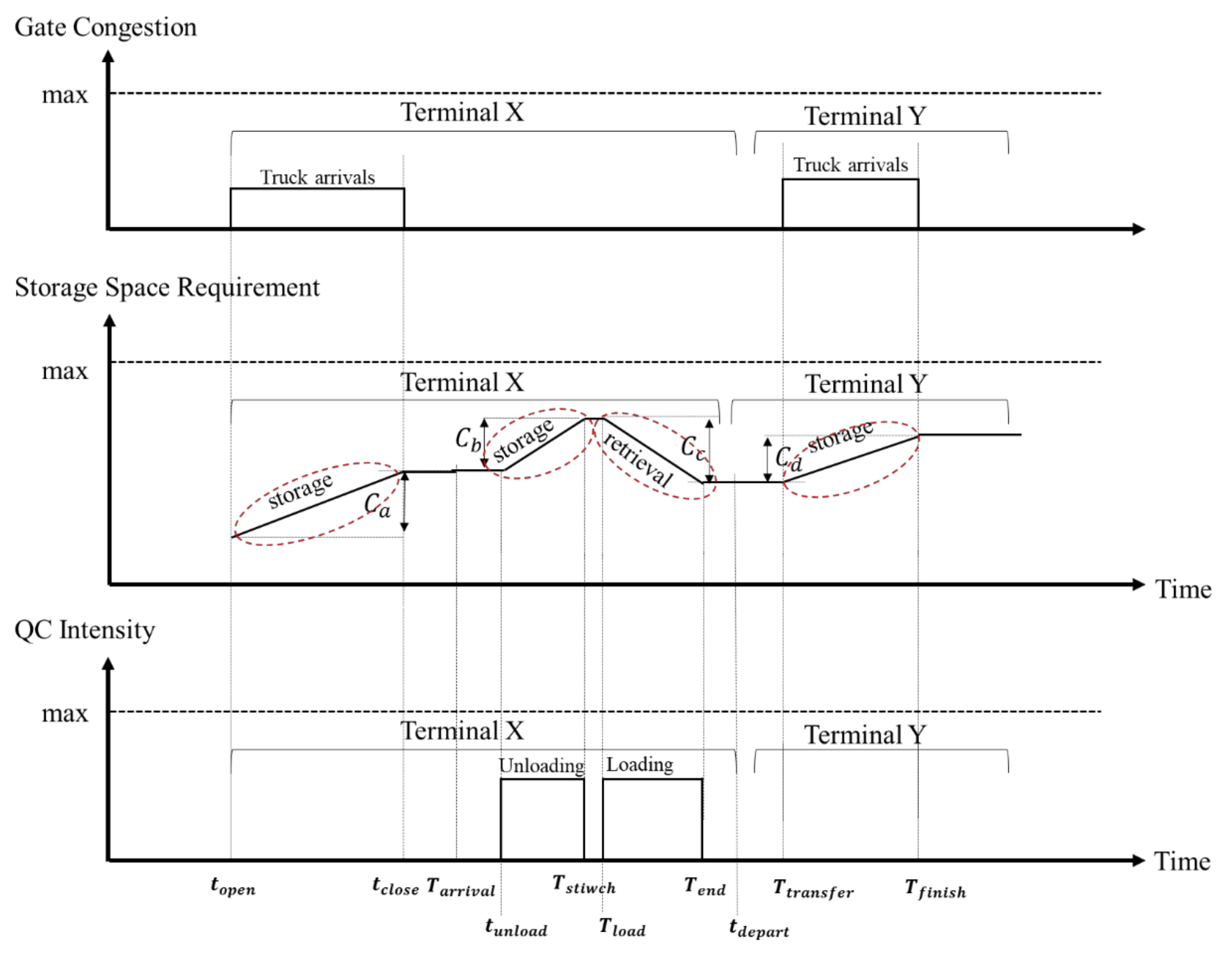
Three major resources in a multiterminal container system are the wharf, gate, and yard. Quay cranes (QCs) on the wharf are interfacing resources between vessels and a terminal; the gates are interfacing resources between the terminal and consignees, and the yards are a representative resource for container storage supporting the operations process across the unloading, loading, receiving, and delivering. A resource profile that considers the varying of the capacity requirements for each type of resource over time-shifts is drawn out. This time-phased resource profile provides a means of estimating the workload on a resource throughout the time-shifts, and thus, assess the capacity adequacy of the system in managing the sporadic demands.

Figure 1 represents the resource profiles of a yard and QCs graphically for two terminals when a vessel arrives at a terminal. The relevant notations are described as follows:

$t_{open}$

= Time for starting the window for outbound or trans-shipment TEUs to arrive at a terminal. It is typically set to two weeks before the expected vessel arrival.

$t_{close}$

= Time for ending the window for outbound or trans-shipment TEUs to arrive at the terminal. It is typically set to one day before vessel arrival.

$T_{arrival}$

= (Random variable) Time that the vessel arrives at the terminal. The ETA of a vessel is nominated when constructing a berth schedule. For purposes of simplicity, this study excludes the berth scheduling, and the vessel arrival is set to follows a probability distribution.

$t_{unload}$

= Time for starting the unloading operations for the vessel. It is typically set to 2 h after vessel arrival.

$T_{switch}$

= (Random variable) Time for switching operation modes. The duration between time when an operation mode is switched and the time when the unloading begins, i.e., $T_{switch}-t_{unload}$, depends on the QC intensity requested by the vessel and the amount of TEUs for the unloading from the vessel.

$T_{load}$

= (Random variable) Time for TEUs to be loaded onto a vessel, transferred to another terminal (if any) or delivered to mainland. Typically, time window $T_{load}-T_{switch}=0$.

$T_{end}$

= (Random variable) Time for completing the loading operation for a vessel. $T_{end}-T_{load}$ also depends on the QC intensity requested by a vessel and the amount of TEUs for the loading operation of the vessel.

$t_{depart}$

= Time for vessel departure. It is typically set to 2 h after the loading completion.

$T_{transfer}$

= (Random variable) Time for TEUs to be loaded onto trucks for transfer to another terminal for trans-shipment on another vessel. Trans-shipment TEUs typically leaves the terminal in 2–3 days after unloading.

$T_{finish}$

= (Random variable) Time that TEUs left the terminal. $T_{finish}-T_{transfer}$ is dependent on the travel time of a truck between the two terminals and the amount of TEUs scheduled to be transferred.

$C_a$

= (Random variable) the amount of TEUs arrived in the terminal before the arrival of the mainline vessel. The actual arrivals of TEU quantity are uncertain but variations are usually minimal.

$C_b$

= (Random variable) the amount of inbound and trans-shipment TEUs unloaded from the mainline vessel. There is uncertainty in the amount of TEUs for unloading with a small variance.

$C_c$

= (Random variable) the amount of outbound and trans-shipment TEUs loaded to the mainline vessel to be transferred to another terminal or delivered to mainland. It is also uncertain with a small variance.

$C_d$

= (Random variable) the amount of TEUs received from transferring operations. It depends on the berth schedule and the TEU information of the corresponding vessel. There is also a small level of uncertainty.

$C_a^f$

= (Random variable) $C_a$ for a feeder vessel.

$C_b^f$ = (Random variable) the amount of inbound TEUs unloaded from the feeder vessel.

$C_c^f$

= (Random variable) the amount of outbound TEUs loaded to the feeder vessel.

Figure 1 depicts the container storage and retrieval activities associated with $C_a$, $C_b$, $C_c$, and $C_d$. The resource profiles for $C_a$, $C_b$, $C_c$, and $C_d$ can be represented by cumulative workload distributions. The QC intensity refers to the number of QCs allocated to a vessel and is conditional upon the vessel category and the TEU quantity. The QC intensity affects the unloading and loading rates, and hence, can be used to represent the workload of QCs at the resource profile. Since the yard is a storage space for containers, the number of containers for the accommodation can be straightforwardly regarded as the workload. The truck queue length is a proxy for gate workload.

When a mainline vessel arrives, the outbound containers from mainland and the transferred outbound containers from other terminals were stacked in the yard in advance (TEU workload in $C_a$). The TEUs from the unloading operations of the vessel temporarily increases the TEU quantity in the yard (TEU workload in $C_b$) as much as the inbound and trans-shipment TEUs. The stacked outbound and transferred containers are loaded onto the vessel and the corresponding TEU quantity (TEU workload in $C_c$) decreases during the loading operation. A part of unloaded containers can be transferred to another terminal (TEU workload in $C_d$) for trans-shipment according to the predetermined berth schedules of the terminals.

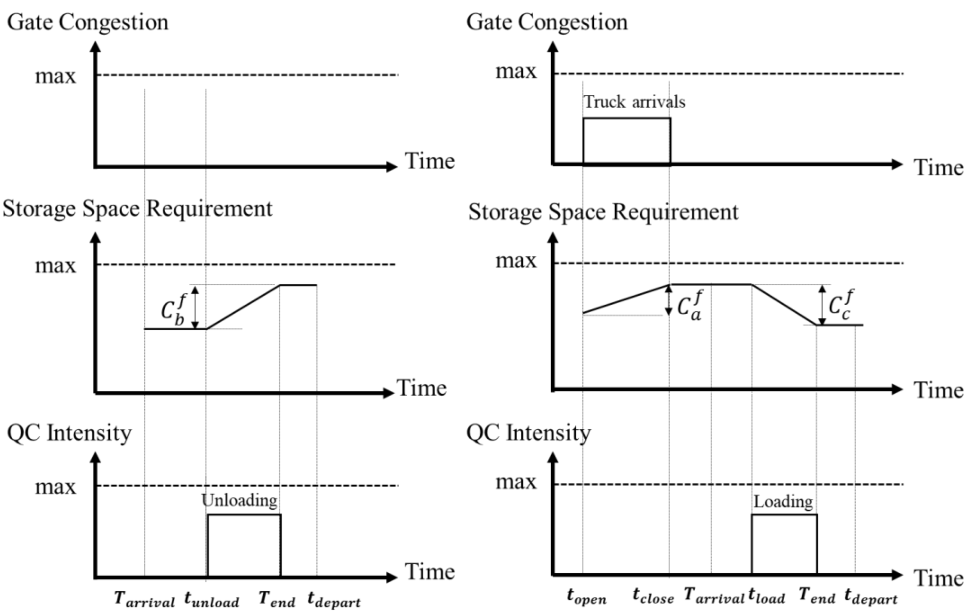
When applying the resource profiles for feeder vessels, as depicted in Figure 2, the resource requirement is relatively simple compared to that of mainline vessels. Since the feeder vessels transport containers plying between trans-shipment and neighboring terminals, there are only unloading and loading operations at a terminal without the need of transferring to another. When a given amount of TEUs are unloaded from a feeder vessel, they are eventually loaded onto a mainline vessel resulting in the increase of TEU quantity in the yard (TEU workload in $C_b^f$). Meanwhile, when a feeder vessel is scheduled to load TEUs from the terminal, a small proportion of total TEUs arrived earlier at the yard (TEU workload in $C_a^f$) from a mainline vessel, and a certain amount of TEUs are loaded onto the feeder vessel (TEU workload in $C_c^f$).

Comparing the unloading and loading processes, the speed of unloading speed is faster at the beginning of operations and subsequently slows down in preparation for the switch to loading operations. The unloading operations, especially for containers on the deck, can usually be done efficiently with a well-designed vehicle dispatching strategy. On the other hand, the loading process is relatively slower because the process needs to consider the loading plan (i.e., terminal-level stowage plan) and ensure the ship’s stability and safety. The loading process are also dependent upon the supporting operations of vehicles and yard cranes that need to be carefully sequenced and dispatched. Meanwhile, the hatch cover handling operations, involving the uncovering and covering of the hatch, increases the durations of both the unloading and loading process as the quay cranes switch the spreader to wired hooks.

2.2. Workload Distributions

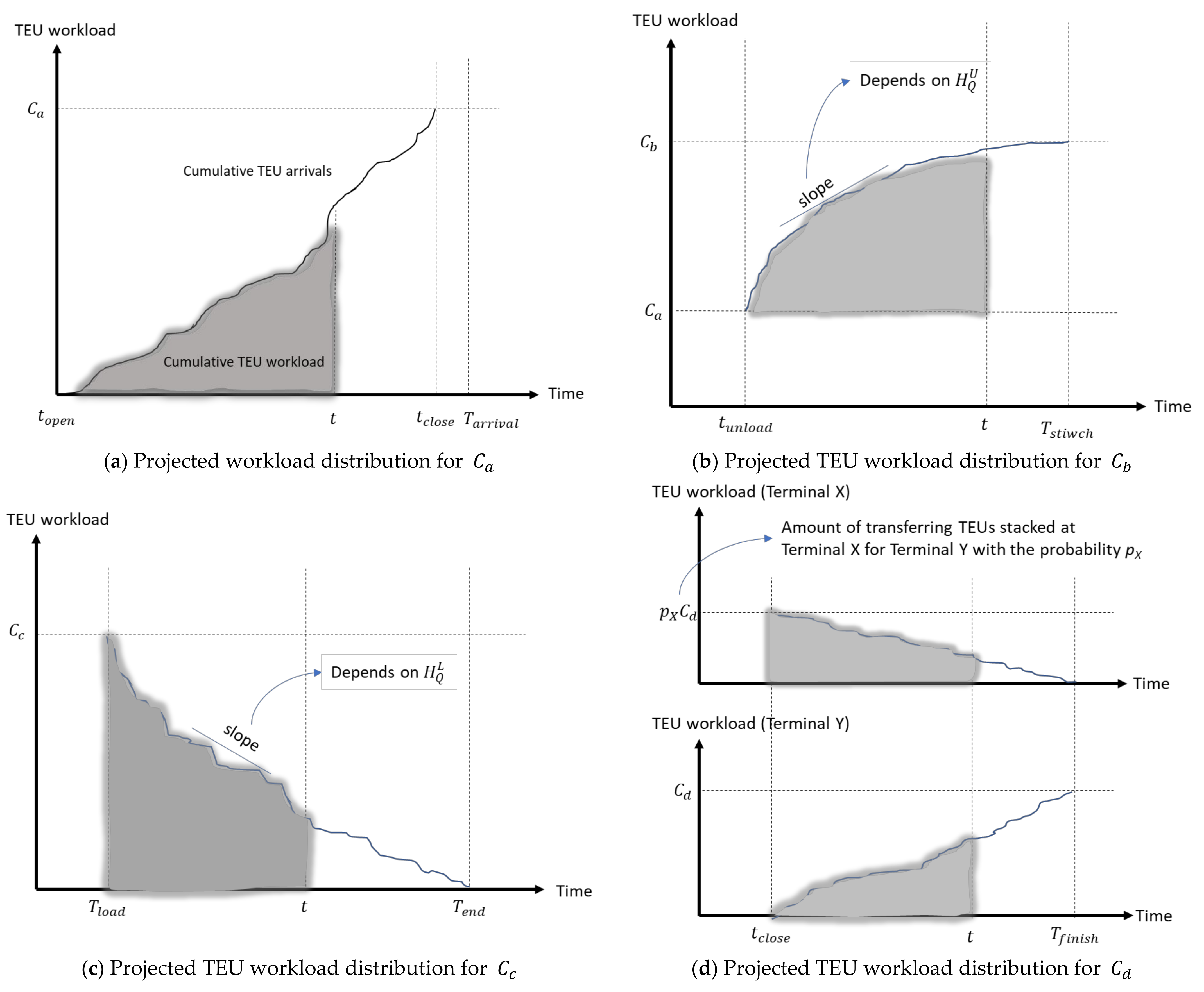
The random variables $C_a$, $C_b$, $C_c$, $C_d$, $C_a^f,C_b^f,$and$C_c^f$ change the workload of the resources over time-shifts. The set of randomness of the random variables, described in the above subsection, also generate probability distributions for requesting workload for storage and retrieval operations as conceptually depicted in the Figure 3.

The cumulative conditional workload distribution for TEU arrivals before the mainline vessel arrival, associated with the random variable $C_a$, is

$$W_{arrival}\left(t_{open}\le t\le t_{close}|T_{arrival}=t_{arrival}\right)={{\displaystyle \sum }}_{i=t_{open}}^{t}E\left[C_a\right]P\left[C_a|T\le i\right],$$

(1)

where $T_{arrival}$ is a random variable with mild variation and $P\left[C_a|T\le i\right]$ is the cumulative distribution of outbound TEU arrivals from $t_{open}$. The cumulative workload distribution is conditioned by $T_{arrival}$ as $t_{open}$ and $t_{close}$ are determined by the realization of $T_{arrival}$. The cumulative conditional workload distribution of the unloading operation is

$$\begin{array}{c}{W}_{unload}\left(T_{switch}-\left(T_{arrival}+t_{unload}\right)\le t|T_{arrival}=t_{arrival}\right)=\\ {{\displaystyle \sum }}_{i=T_{arrival}+t_{unload}}^{t}E\left[C_b\right]P\left[C_b|T\le i\right]=min\left(\left(t-i\right)H_Q^U,E\left[C_b\right]\right),\end{array}$$

(2)

where $H_Q^U$ is the random variable for the QC gross productivity of a vessel during the unloading operation measured by the amount of TEUs handled per time unit. $P\left[C_b|T\le i\right]$ is replaced with the time-independent unloading rate. The gross productivity is dependent on the QC intensity, which in turn depends on the vessel size and the TEU volume. Hence, $H_Q^U=h_Q^U{I}_Q$, where $h_Q^U$ is the gross productivity distribution of a QC for a vessel for the unloading operation, which can be realized by the number of moves per time unit. For S being a random variable with a small deviation for the vessel category, $I_Q=F_{\left(C_b+C_c,S\right)}$ is the QC intensity distribution for the vessel operation that varies with the amount of TEUs and the vessel size as summarized in Appendix A. Accordingly, the cumulative conditional workload distribution for the loading operation is given as,

$$\begin{array}{c}{W}_{load}\left(T_{end}-T_{load}\le t|T_{load}=t_{load}\right)={{\displaystyle \sum }}_{i=T_{load}}^{t}E\left[C_c\right]P\left[C_c|T\le i\right]=\\ min\left(\left(t-i\right)H_Q^L,E\left[C_c\right]\right),\end{array}$$

(3)

where $H_Q^L=h_Q^L{I}_Q$. $h_Q^L$ is the gross productivity distribution for the loading operations. Note that the workload for the loading operation take a positive effect on reducing the storage space requirement but it requires handling effort to be performed. As for the transferring operations from a terminal to another, the cumulative conditional workload distribution is

$$\begin{gathered} W_{transfer}\left(T_{finish}-T_{transfer}\le t|T_{transfer}=t_{transfer}\right) \\ ={{\displaystyle \sum }}_{i=T_{transfer}}^{t}E\left[C_d\right]P\left[C_d|T\le i\right], \end{gathered}$$

(4)

where $P\left[C_d|T\le i\right]$ represents the transferring productivity of trucks that transport TEUs out to other terminals including the traffic congestion and the gate process. $T_{transfer}$ should correspond to the $t_{open}$ for another vessel incoming to another terminal (Terminal 2 in Figure 1).

The same goes for the workload distributions $C_a^f$, $C_b^f$ and $C_c^f$ of the feeder vessels in Figure 2. The cumulative conditional workload distribution for the unloading operation of a feeder vessel is

$$\begin{gathered} W_{unload}^f\left(T_{end}-\left(T_{arrival}+t_{unload}\right)\le t|T_{arrival}=t_{arrival}\right)= \\ {{\displaystyle \sum }}_{i=T_{arrival}+t_{unload}}^{t}E\left[C_b^f\right]P\left[C_b^f|T\le i\right]=min\left(\left(t-i\right)H_Q^U,E\left[C_b^f\right]\right), \end{gathered}$$

(5)

where $H_Q^U=h_Q^U{I}_Q$ consisting of the gross productivity distribution of a QC for a feeder vessel during the unloading operation $h_Q^U$ and the QC intensity distribution dependent on the amount of TEUs and the feeder vessel size $I_Q=F_{\left(C_b^f+C_c^f,S\right)}$. For a feeder vessel requiring only the loading operation, the cumulative conditional workload distribution for TEU arrivals for a feeder vessel is

$$W_{arrival}^f\left(t_{open}\le t\le t_{close}|T_{arrival}=t_{arrival}\right)={{\displaystyle \sum }}_{i=t_{open}}^{t}E\left[C_a^f\right]P\left[C_a^f|T\le i\right]$$

(6)

The cumulative conditional workload distribution for the loading operation of a feeder vessel is

$$\begin{gathered} W_{load}^f\left(T_{end}-\left(T_{arrival}+t_{load}\right)\le t|T_{arrival}=t_{arrival}\right)= \\ {{\displaystyle \sum }}_{i=T_{arrival}+t_{load}}^{t}E\left[C_c^f\right]P\left[C_c^f|T\le i\right]=min\left(\left(t-i\right)H_Q^L,E\left[C_c^f\right]\right), \end{gathered}$$

(7)

where $H_Q^L=h_Q^L{I}_Q$ consisting of the gross productivity distribution of a QC for the loading operation $h_Q^L$.

2.3. Resource Profile Simulation

A resource profile simulation is developed to generate events imposing workload requirement for resources, such as vessel arrivals, truck transportation, loading and unloading operations, etc. presented in Figure 4, and simulate the workload cascading over the resources across terminals. The events are associated with the random variables provided in the previous section and each event triggers another. The resource profiles simulation estimates the workload distributions for resources to estimate the capacity requirement over time-shifts across the terminals.

• ${\mathit{E}}_{\mathit{a}}\left(\mathit{i},\mathit{x}\right)$-Vessel arrival. This event is triggered when a vessel with type $i$ arrives at the port and randomly assigned to any of one of the terminals $x\in M$ with an equal probability, where $M$ is the set of cooperative terminals at the port. The vessel type is characterized by the attributes such as the category, the TEU quantity, the required QC intensity. When the event is executed, the attributes of the vessel are randomly assigned by referring to Appendix A. The event triggers an immediate execution of $E_u$, $E_t$, and $E_s$ and schedule a new event $E_a\left(i,x\right)$ with an exponential interarrival rate $\lambda$. This event is associated with the workloads $C_a$ and $C_a^f$.
• ${\mathit{E}}_{\mathit{t}}$-TEU arrival. This event is triggered when a vessel arrives at the port. The arrivals of TEUs was recorded earlier than the time of executing $E_a$ by tracing back in time. The workload $C_a$ is distributed only in the time ranged from $t_{open}$ to $t_{close}$. Both $t_{open}$ and $t_{close}$ are dependent on the generated $T_{arrive}$.
• ${\mathit{E}}_{\mathit{u}}$-Unloading. This event is triggered when the first vessel in the queue arrives at a randomly selected terminal. The event execution time is delayed until $t_{unload}$ as both the vessel and the QCs operations must be ready for the unloading operations (which generally takes 2 h) to be performed. The event allocates QCs to the vessel as requested (generated) in the event of $E_a$. It is set that the required number of QCs is always available at a terminal. The time window for the unloading operation $T_{switch}-t_{unload}$ is conditionally determined by the generated $H_Q^U$. When the event is triggered, the amount of TEUs in the yard increases at the rate of $H_Q^U$. The workloads $C_b$ and $C_b^f$ are associated with the event. The simulator sets unloaded TEUs to leave the terminal within 5 days following the unloading. The unloading event $E_u$ triggers the execution of the loading event $E_l$ through determining $T_{switch}$.
• ${\mathit{E}}_{\mathit{l}}$-Loading. The event is triggered immediately upon the completion of the unloading operation on the vessel. $T_{switch}$ is used to execute the loading event $E_l$ but the event execution time is delayed until $T_{load}$. Similar to the unloading operation, the loading time window $T_{end}-T_{load}$ is conditionally determined by the generated $H_Q^L$while the TEUs at the yard also decreases accordingly. The workloads $C_c$ and $C_c^f$ are adjusted with the event. The event triggers the execution of the vessel departure event $E_d$ though determining $T_{end}$.
• ${\mathit{E}}_{\mathit{d}}$-Vessel departure. The execution time of this event is delayed until $t_{depart}$, which is determined by the generated $T_{end}$ as the both the vessel and the QCs operations must be ready to be released. When executing this event, the vessel returns the assigned number of QCs, releases the quay space of the terminal, and triggers an immediate execution of $E_a$.
• ${\mathit{E}}_{\mathit{s}}$-TEU Transfer. This event is triggered when the event of vessel arrival $E_a\left(i,y\right)$ where $y\in M\backslash \left\{x\right\}$ is executed. The event generates $C_d$ over the time window $T_{finish}-T_{transfer}$ for interterminal trans-shipment at each cooperating terminal, with the time window for trans-shipment TEUs being 2–3 days after unloading at a terminal. Hence, the TEU transferring activities are recorded earlier than the time of executing $E_a\left(i,y\right)$. $T_{transfer}$ is generated by the execution of $E_a\left(i,y\right)$ and $T_{finish}$ is dependent on the transferring productivity of trucks.
• ${\mathit{E}}_{\mathit{t}}$-Truck transport. This event is triggered when $E_a\left(i,y\right)$ determines $T_{transfer}$. An amount of TEUs at a terminal, $C_d$, will need to be transported to terminal $y$ from $x$ by trucks. A generated single truck typically transports 1.5 TEUs at a time. When a truck transports transferring TEUs from a terminal to another, the process takes a number of time-units including the congestion on traveling paths. The congestion has the effect of reducing the speed of truck flows. Underwood formula is used to adjust the truck speed for the traffic congestion on a traveling path, taking into account parameters such as length of the travel path, free flow speed, and a predetermined amount of maximum number of trucks. The effective traveling speed $u_n$ in a traveling path between two terminals with $n$ trucks is estimated by

  $$u_n=u_{f}exp\left(-\frac{k_n}{k_0}\right),$$

  (8)

  where$u_f$ is the free speed and$k_0$ is the traffic density at maximum flow. For $L^t$ representing the length of the traveling path, $k_n=\left(n-1\right)/L^t$is the traffic density in the traveling path with $n$ trucks. The event triggers an immediate execution of $E_g$ with the delay of traveling and congestion of a truck.
• ${\mathit{E}}_{\mathit{g}}$-Gate check-in. The execution time of this event is delayed until the arrival of a truck, as the traveling time and delays caused by congestion should be included. Since the gate is a resource with limited capacity, the queue length will be a meaningful measure for gate workload. The gate is modeled as a single server machine and its service times are adjusted for multiple pass lanes. Whenever a truck arrived at a gate (i.e., the execution of $E_g)$, it joins the gate queue and waits for the check-in service. The truck queue length is affected by the workload distribution of Equation (4) and counted as the gate congestion measure in the simulation. The gate check-in event triggers an immediate event $E_c$.
• ${\mathit{E}}_{\mathit{c}}$-Arrival of Transferred TEU. This event is triggered when a truck passes the gate, but the execution time is deferred until the truck is processed at the gate. It increases the TEU workload in the yard accordingly at most $C_d$. This event generates $T_{finish}$, and calls the event $E_s$ to transport TEUs continuously until cumulative probability for TEU workload, $P\left[C_d|T\le i\right]$, becomes 1. Transferring time window $T_{finish}-T_{transfer}$ essentially includes the two delay elements, namely, congestion and queueing that increase uncertainty.

3. Simulation Experiment

A set of simulation experiment is conducted to understand the capacity requirements for different volumes of trans-shipment ratios of containers relative to inbound and outbound containers at a terminal, as well as different transferring container volumes across terminals. The base-case setting is as follows: four equal-size of terminals located at a trans-shipment hub port are sharing the resources. Each terminal has 1000 m quay length and initial inventory at the yard is 20,000 TEUs. The distance between adjacent terminals is set to 500 m, and the terminals are sequentially laid in a line. The truck free speed in between terminal is set to 14 m/s. The traffic density at maximum flow ($k_0$) in the Underwood formula is calculated by setting the effective speed under jammed traffic ($u_{N_{max}}$) to 0.01 m/s, where the maximum number of trucks ($N_{max}$) for transferring activities between terminals is limited to 25. The gate service time is preset to follow $U\left(5,10\right)$ min. This service time measures the duration-of-stay of a truck in the boundary of gate system and includes the time spent on checking the driver identification, truck number, container number, and measuring the weight, temperature (for reefer), and size (for out-of-gauge) of the container and deciding a storage slot for the container. Additionally, when the container door is not facing outward, a reach stacker needs to turn the direction of the container.

To avoid the situation whereby insufficient resource capacity leads to a distortion in the actual capacity requirement reflected in the resource profile, the study assumed that the requested QC intensity of every vessel can be met. The QC intensity is determined by the vessel category (size) and the TEU quantity on the vessel described in Appendix A. The vessel and TEU categories in the experiment is drawn upon their respective pools based on a uniform distribution. The gross productivity of a QC is assumed to be normally distributed, $N\left(28,4^2\right)$, hourly. $t_{open}$ and $t_{close}$ are set to 2 weeks and 1 day, respectively, and the vessel arrival $T_{arrival}$ is set to follows exponential interarrival time with a mean of 2.05 hourly. $t_{unload}$ is set to 2 h after the vessel arrival. It is further assumed that the incoming vessels arrive at any terminal with equal probabilities. The probability that an arriving vessel is a mainline vessel is 90%, while the probability of receiving a feeder vessel is 10%. When the latter occurs, half of these vessels are for unloading and the other half for loading only (note: this contrasts with the mainline vessel which will first perform the unloading operations and then the loading operations). The terminals have equal probabilities to be selected when transferring the trans-shipment TEUs to them.

The simulation scenarios are represented by varying the rates of transshipment and outbound and inbound TEUs, as well as the rates for which the trans-shipment TEUs would remain in its arrival terminal or be transferred to other terminals. The simulation runs 10 replications for each setting for 200 days after the warming-up period. Since the warming-up period depends on experiment settings, the simulation results are sampled out after eliminating the initialization bias by shown in the output plots. The simulation model is implemented using C# programming language as part of the Visual Studio Community 2017 and run on a computer with Intel processor i5, 1.8 GHz with 16 GB RAM.

3.1. Simulation Results with Low Transferring

The proportion of TEUs for inbound and trans-shipment-inbound are set to 20% and 80%, respectively, and the same proportion applies to the TEUs for outbound and transshipment-outbound. The proportions of TEUs remaining in a terminal and transferring to the other terminals are set to 40% and 60%, respectively. All the other terminals have equal probabilities to take the transferred TEUs and the transferring is only limited to trans-shipment TEUs.

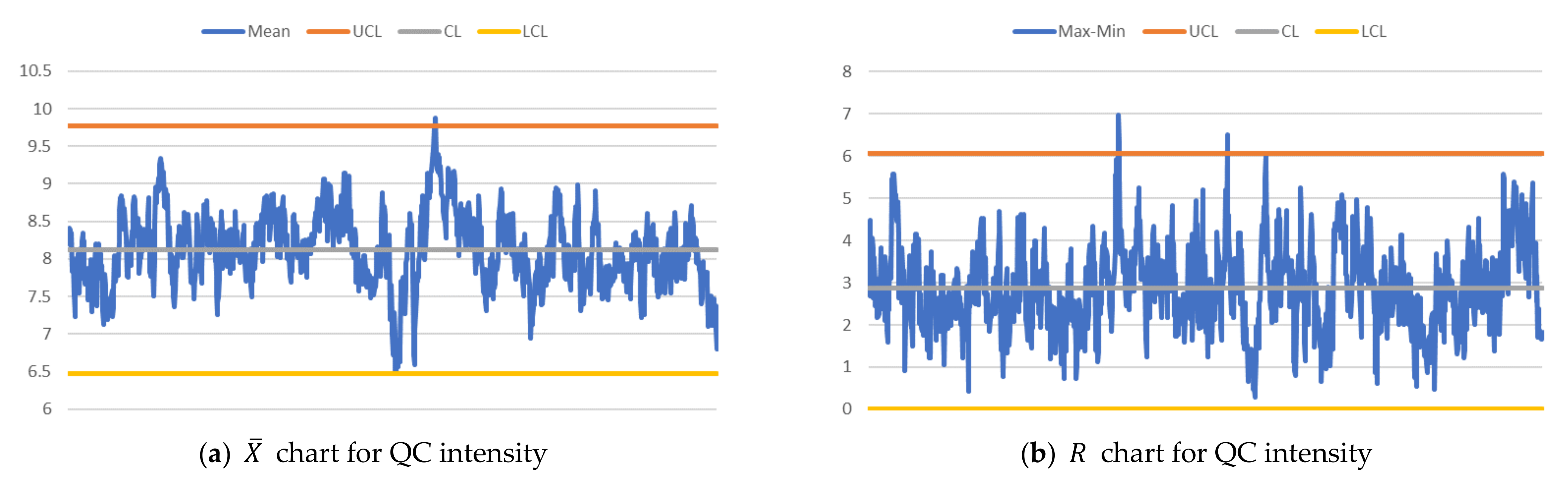
Based on the collected samples, $\overline{X}-R$ Charts for QC intensity, the TEU workload at the yard, and the queue length at the gate can be drawn with the estimated control limits consisting of upper control limits (UCLs), central lines (CLs), and lower control limits (LCLs) for each set of output [21]. Specifically, the simulation plots the QC intensities currently serving all vessels at the terminal whenever a vessel leaves a terminal ($E_d$). 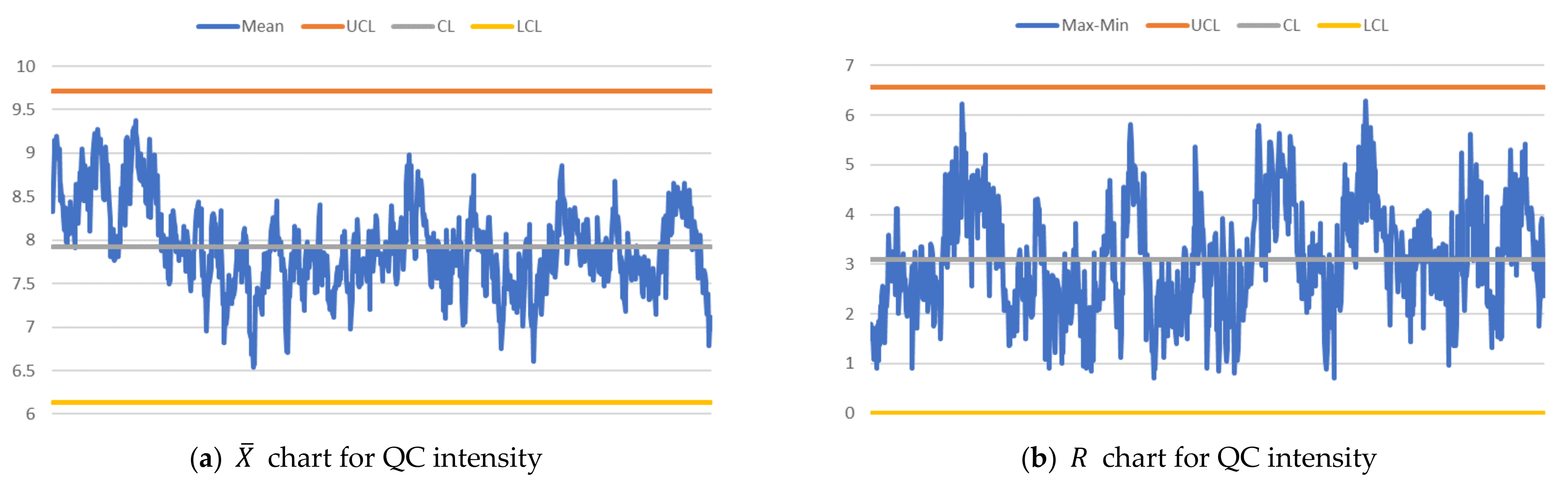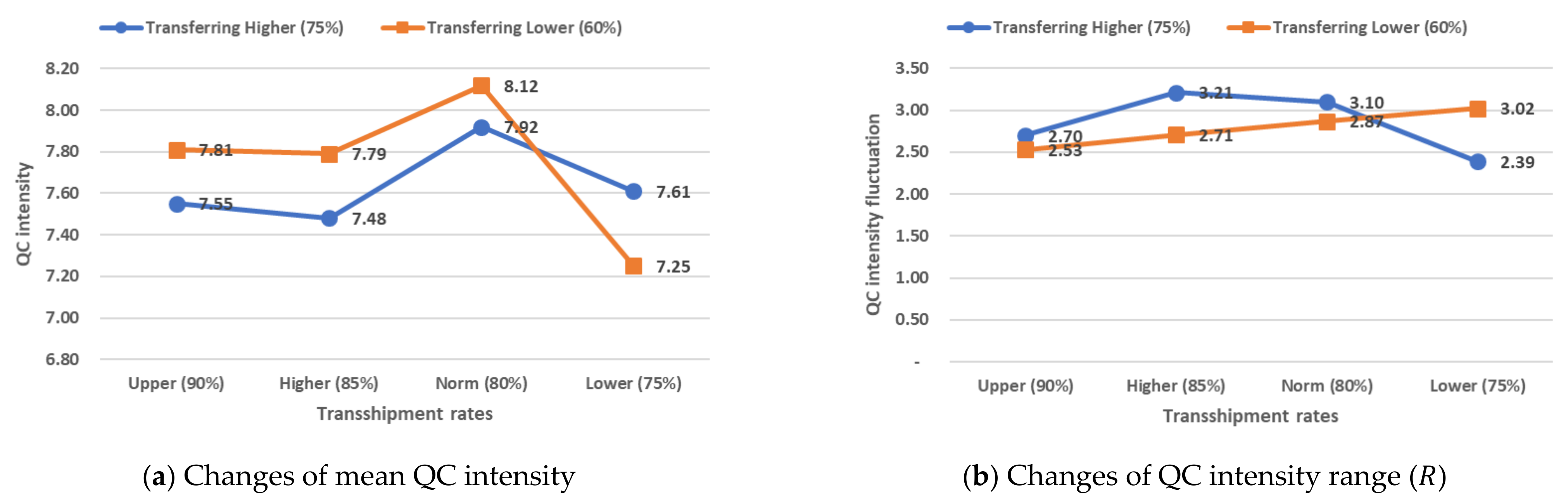Figure 5 shows the simulation results of QC intensities over time-shifts. The mean requirement of QC intensity for vessel service is 8.12 and the upper limit is estimated as 9.78. It means that a terminal needs to prepare 9.78 QCs to meet the handling capacity requested by the incoming vessels, even though on average only 8.12 QCs are needed to meet the capacity request.

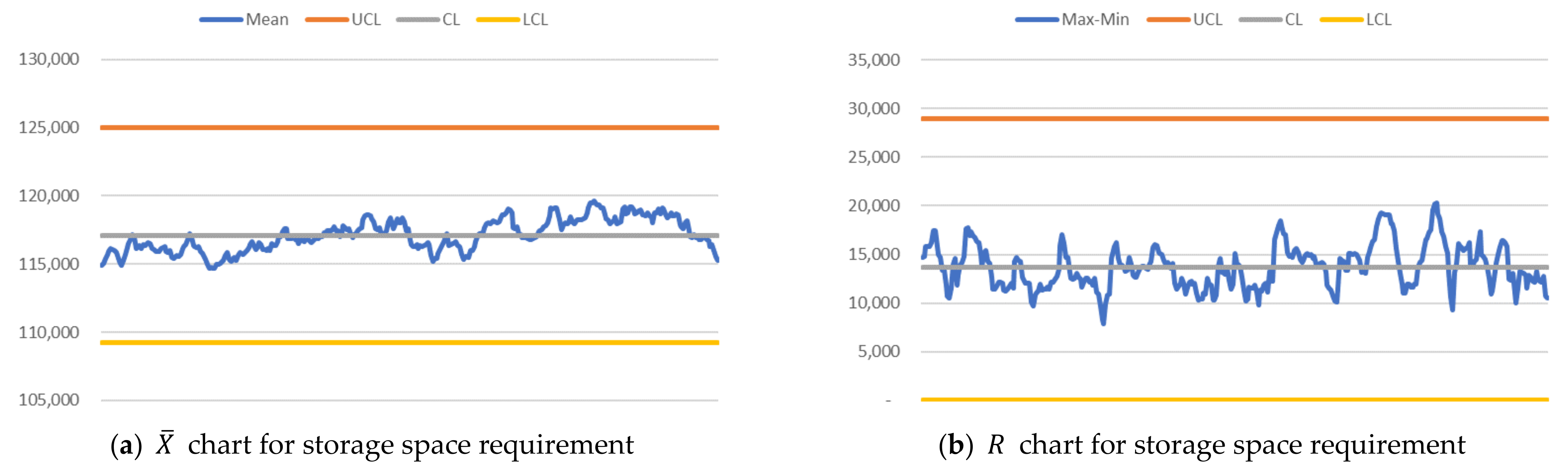
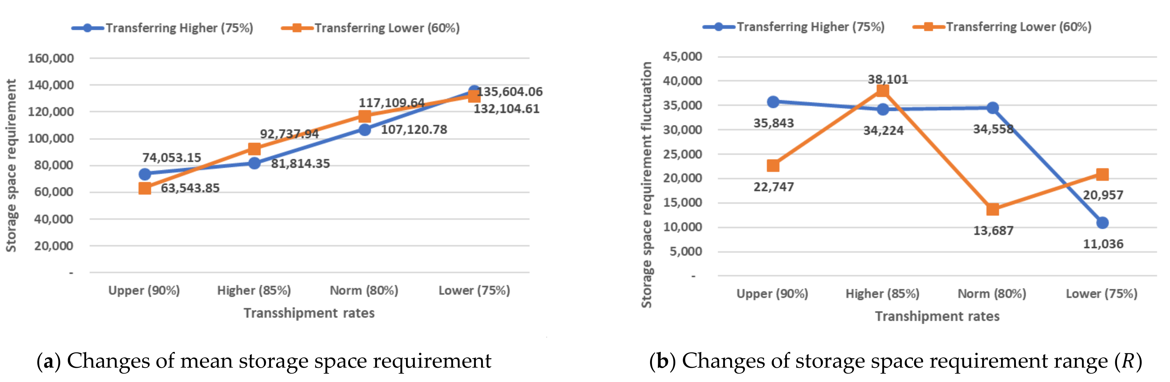
The storage space requirement in TEUs is plotted when any of these three events takes place: (i) a vessel arrives at the terminal ($E_a$); (ii) the interterminal transferring is completed ($E_c$), and (iii) a vessel departs ($E_d$). Figure 6 shows that the mean storage capacity required to support the requested vessel service is estimated to be 117,109.64 TEUs, with 125,006.81 and 109,212.50 TEUs as the upper and lower control limits, respectively. The mean difference between maximum and minimum storage requirements is estimated as 13,686.60 TEUs.

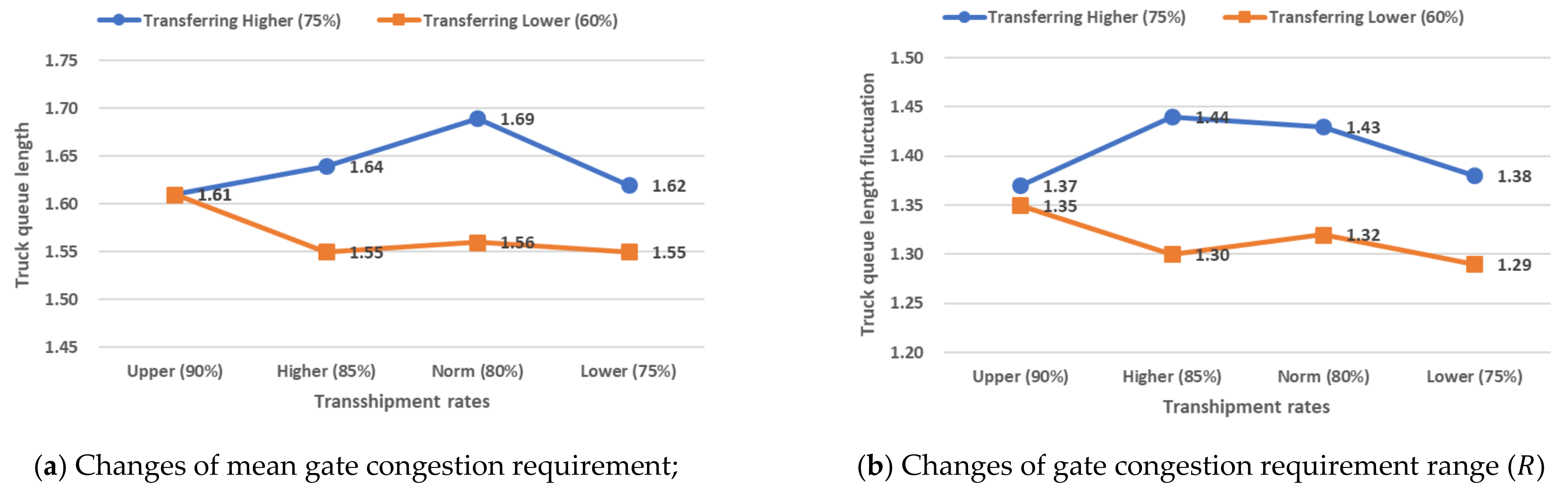
Gate availability is critical for the smooth execution of interterminal transferring activities. A long truck queue is usually an indication of gate congestion. Figure 7 plots truck queue length at every instance when a truck reaches the gate ($E_g$). The estimated queue length is 1.56 trucks, and the upper limit shows 2.32 trucks in the queue. Thus, it can be inferred that the gate needs to possess adequate capacity to clear an average queue length of 1.56 trucks to provide the handling service requested by vessels during the transferring activities. Note that the truck queue is estimated only for transferring containers. The results are summarized in

Table 1. Control limits of $\overline{X}-R$ charts for QC intensity, storage space requirement, and gate congestion corresponding to Figure 5, Figure 6 and Figure 7.

		$\overline{\mathit{X}}$ Charts			$\mathit{R}$ Charts
	UCL	CL	LCL	UCL	CL	LCL
QC intensity	9.78	8.12	6.47	6.06	2.87	0
Storage space requirement	125,006.81	117,109.64	109,212.50	28,933.48	13,686.60	0
Gate congestion	2.32	1.56	0.79	2.80	1.32	0

.

3.2. Simulation Results with High Transferring

A parallel experiment is conducted to examine the effect of a high transferring TEUs rate. The proportions of TEUs remaining in a terminal and transferring to the other terminals are set to 25% and 75%, respectively. The proportion of TEUs for inbound, trans-shipment-inbound, outbound, and transshipment-outbound remains to be same as Section 3.1. The simulation results are drawn in Figure 8, Figure 9 and Figure 10 using $\overline{X}-R$ Charts and summarized in

Table 2. Control limits of $\overline{X}-R$ charts for QC intensity, storage space requirement, and gate congestion corresponding to Figure 8, Figure 9 and Figure 10.

		$\overline{\mathit{X}}$ Charts			$\mathit{R}$ Charts
	UCL	CL	LCL	UCL	CL	LCL
QC intensity	9.71	7.92	6.13	5.65	3.10	0
Storage space requirement	127,060.92	107,120.78	87,180.64	73,056.25	34,558.30	0
Gate congestion	2.52	1.69	0.86	3.03	1.43	0

.

The simulation results of QC intensities for all vessel arrivals over the run-time suggest that a terminal is expected to prepare 9.71 QCs if it wishes to meet the handling capacity requested by the incoming vessels entirely, but on average 7.92 QCs are sufficient to meet the capacity request (Figure 8). The QC intensity is generally lower than what was found previously in Section 3.1. It indicates the workload in the quayside operation will be reduced by 2.5% when the transferring rate increases from 60% to 75%.

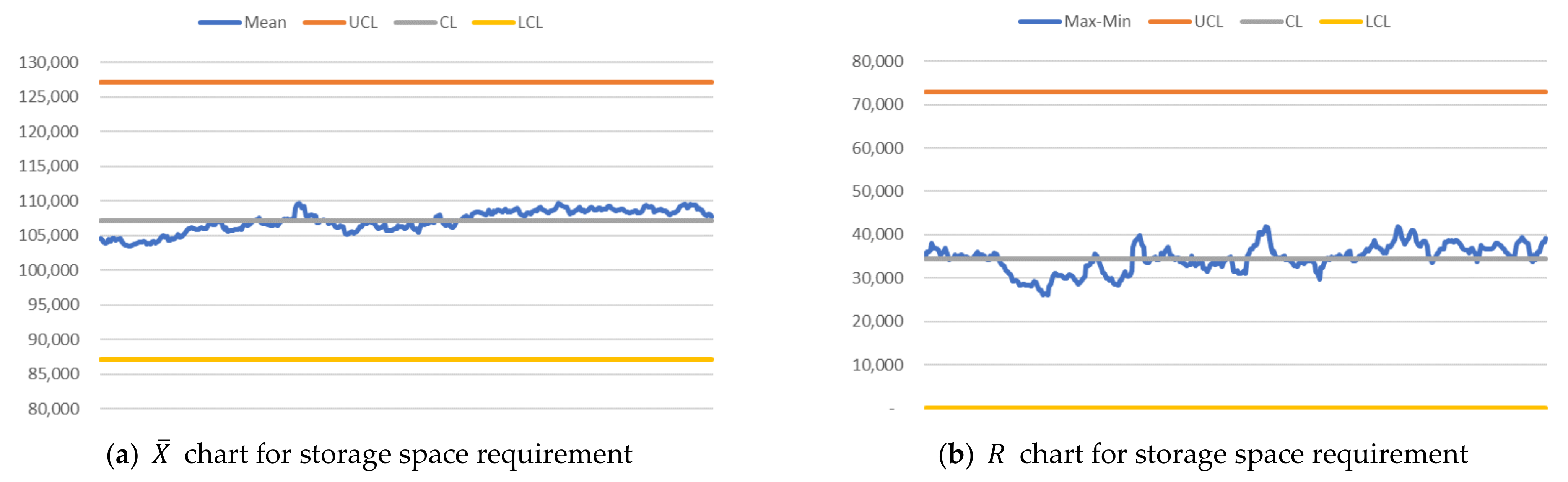
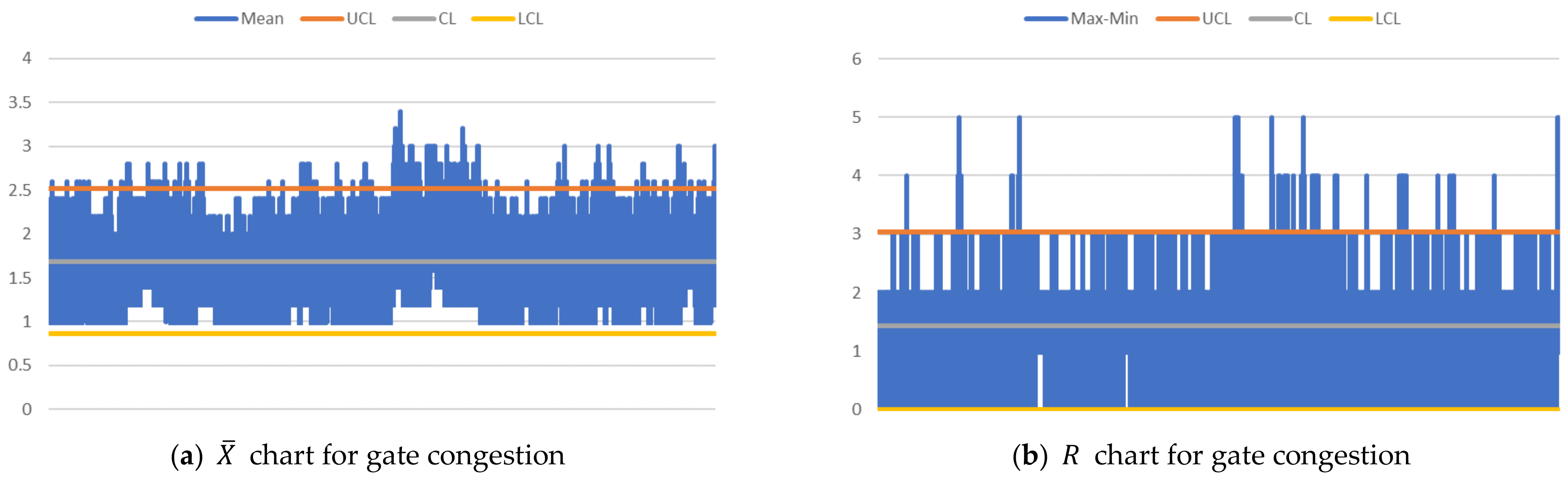
Figure 9 shows that the mean storage capacity requirement to support the requested vessel service is estimated to be 107,120.78 TEUs, with 127,060.92 and 87,180.64 TEUs as UCL and LCL, respectively. Compared to the results in Section 3.1, the increase of transferring rate has helped reduce the storage capacity requirement by 8.5% on average. However, the gap between the two limits has also widened by 152.5% at the same time. This widened gap indicates increased variation of storage capacity requirement with the mean difference between maximum and minimum storage requirements estimated at 34,558.30 TEUs. Meanwhile, the estimated truck queue length is 1.69 trucks with 2.52 in UCL for transferring TEUs (Figure 10). The gate processing requirement is increased by 8.3% in terms of the mean queue length as the transferring TEUs increase.

4. Managerial Insights

The simulation results in Section 3 gives the capacity requirements for a range of setting of transferring TEUs rates across terminals when each terminal handles a combination of inbound, outbound, and trans-shipment TEUs. This section further discusses the managerial insights over various combinations of TEU workload requirement for multiterminal cooperation.

4.1. Analysis on Workload Significance

In the previous section, the simulation results are obtained under the experimental setting of 80% trans-shipment TEUs and the remaining 20% equally split into inward-bound and outward-bound TEUs. This forms the base model for comparison.

Further experimental analysis allows the summation of equal inbound and outbound TEU rates to be determined by the TEU rate for transshipment, i.e., the larger the percentage of trans-shipment TEUs, the lower the aggregate inbound and outbound TEUs. Similarly, the rate for TEU remaining in a terminal is also dependent upon the transferring rate to other terminals since both rates must sum to 1. As before, only trans-shipment TEUs can be transferred, and the other terminals have equal probabilities to take up the transferred TEUs. The purpose of this extended analysis is to understand the effects of the relative volumes of trans-shipment containers against those of the inbound and outbound containers and the volumes of transferring containers across terminals on the capacity requirement.

The four levels of the trans-shipment rates (i.e., Upper-90%, Higher-85%, Norm-80%, and Lower-75%) and the two levels of the interterminal container transferring (i.e., Higher-75% and Lower-60%) are simulated. Each combination has a sample of size 200. It means that 200 time-points of vessel departures are randomly selected from the simulation results and the relevant dataset (for the selected 200 time-points) for the QC intensity, the storage space requirement, and the gate congestion is taken. The summarized descriptive statistics are presented in Appendix B.

Figure 11a compares the mean QC intensities across the trans-shipment rates and the transferring rates. From the figure, the QC intensity is increased by 4.1% and 12% when transferring rates are at a high and low of 75% and 60%, respectively, when the trans-shipment rate is increased up to 80% from 75%. The increase in QC intensity is logical, as the shortened duration-of-stay of containers at yard increases higher handling request at the quayside. The smaller increment observed under the higher transferring rate is due to the higher support of distributing workload by means of transferring. Further increase to the trans-shipment TEUs rates (for example, 85%) leads to 5.6% and 4.1% reduction of QC intensity under higher and lower transferring rates, respectively. This reduction can be attributed to the possibility of transferring workload to other terminals, which in turn, translates into better chances for a more evenly distributing QC handing workload across terminals. Subsequent increase in the trans-shipment rate to 90% produces an increase of QC intensity by nearly net of 0.9 and 0.3%, respectively. At this level of trans-shipment rate, the workload distribution effect of transferring work is dominated by the even higher handling request for QCs.

Another important element concerns the uncertainties in resource requirements. As shown in Figure 11b, despite having a high level of the trans-shipment rate (i.e., 90%) that provides opportunities to reduce QC intensity through TEUs redistribution across terminals, higher uncertainty in QC intensity requirement is reported when there are active transferring activities among the terminals (i.e., transferring rate at 75%). On the other hand, the lower transferring rate (i.e., 60%) contributes to the monotonic decreases of QC intensity as the trans-shipment rate increases.

When the trans-shipment rates are reduced, the corresponding rates for outbound and inbound TUEs increase. This leads to longer expected duration-of-stays for TEUs at the yard and increasing storage space requirement (Figure 12a). When the transferring TEUs rate to other terminals is lowered from 75% to 60%, the terminal will require a 1.5% higher storage space capacity on average as more space is needed to accommodate containers at the yard. However, as the trans-shipment rate rises up to 90%, the storage space capacity associated with the lower transferring rate (60%) drops by 14.2%. While the shortened expected duration-of-stays associated with the high rate of trans-shipment TEUs (i.e., at 90%) leads to the reduced storage space capacity requirement, the higher rate of transferring TEUs increases the requirement for storage space capacity to put up incoming containers (thereby producing an offsetting effect for storage space capacity savings). The offsetting effect revisits when the trans-shipment rate is lowered to 75% leading to the storage space requirement increases to nearly 2.6%.

Figure 12b shows that the requirement uncertainty on storage space is somewhat unaffected when the trans-shipment rate decreases from 90% to 80%. The requirement uncertainty on storage space saw a sharp drop of 68.1% with further reductions in the trans-shipment rate from 80% to 75% under the higher transferring rate of 75%. As the trans-shipment rate falls, the expected duration-of-stays for TEUs at the yard lengthens and reduces the requirement uncertainty though the higher transferring rate (i.e., 75%) works in the opposite direction. Further reduction of trans-shipment rate (i.e., 75%) magnifies the uncertainty reduction of storage space requirement with longer duration-of-stays for TEUs. The requirement uncertainty on storage space is much variable for the trans-shipment rates when the transferring rate is lower (i.e., 60%). Overall, there is a tendency towards the declination of the requirement uncertainty when the trans-shipment rate decreases for the same reason as that of the higher transferring rate.

The truck queue length is generally shorter when the rate of trans-shipment TEUs and interterminal rates of transferring TEUs are low (Figure 13a). On the contrary, under the higher transferring rate, increasing the rate of trans-shipment TEUs results in increased traffic congestion on the path transporting containers between terminals. This leads to a reduction in arrival rate of trucks which, in turn, results in an average 2.4% reduction in queue length at the gate. When the trans-shipment rate is decreased to 75%, the traffic congestion is less effective in alleviating gate congestion. Instead, a reduced amount of trans-shipment TEUs transferred is shown to be more effective in reducing the truck arrival rate with the truck queue at the gate being shortened by 4.1%. The plot of gate congestion range in Figure 13b behaves very similarly to that of queue length in Figure 13a since the uncertainty on truck queue is attributed to the traffic congestion for trucks transporting containers between terminals, as well as the arrival rate of trucks at the gate. Variations of truck queues at the gates decrease with a shorter average queue length and increase with a longer queue of trucks.

4.2. Analysis on Interaction Effects

A two-factor ANOVA with replications is applied to examine the effect of trans-shipment and transferring rates on capacity requirement of QC intensity (

Table 3. Two-factor ANOVA results for QC intensity in 5% significance level.

	Sum of Square (SS)	Degree of Freedom (df)	Mean Sum of Square (MS)	F-Ratio	p-Value	Significance (Sig.)
Trans-shipment	140.07	3	46.69	266.66	3.22 × 10−140	yes
Transferring	23.03	1	23.03	131.53	2.60 × 10−29	yes
Interaction	61.14	3	20.38	116.39	3.82 × 10−68	yes
Error	278.75	1,592	0.18
Total	502.99	1,599	0.31

), storage space requirement (

Table 4. Two-factor ANOVA results for storage space requirement in 5% significance level.

	SS	df	MS	F-Ratio	p-Value	Sig.
Trans-shipment	989,432,180,454.49	3	329,810,726,818.16	237,253.37	0	yes
Transferring	1,716,883,011.15	1	1,716,883,011.15	1,235.06	9.21 × 10−201	yes
Interaction	30,685,348,400.53	3	10,228,449,466.84	7,357.96	0	yes
Error	2,213,071,537.21	1,592	1,390,120.31
Total	1,024,047,483,403.38	1,599	640,429,945.84

), and gate congestion (

Table 5. Two-factor ANOVA results for gate congestion in 5% significance level.

	SS	df	MS	F-Ratio	p-Value	Sig.
Trans-shipment	26.05	3.00	8.68	195.78	4.58 × 10−108	yes
Transferring	4.62	1.00	4.62	104.24	9.50 × 10−24	yes
Interaction	21.74	3.00	7.25	163.44	2.35 × 10−92	yes
Error	70.60	1,592.00	0.04
Total	123.01	1,599.00	0.08

). The p-values reject the null hypothesis in favor of the alternative hypothesis and conclude that the difference in trans-shipment rates has an effect on the QC intensity, storage space requirement, and gate congestion at the 95% significant level. The same applies for the transferring rates and the interaction effect of trans-shipment and transferring rates.

The ANOVA contrast determines whether there is a significant difference in levels of the QC intensity, the storage space requirement, and the gate congestion when the factor levels (i.e., transferring and trans-shipment rates) vary. The number of contrast coefficients is set to 2, and Bonferroni correction is applied when testing the significance between levels of a factor.

Table 6. Significance test among trans-shipment levels for QC intensity, storage space requirement, and gate congestion using contrasts at 5% significance level.

		Higher (85%)	Norm (80%)	Lower (75%)
QC intensity	Upper (90%)	no	yes	yes
	Higher (85%)	-	yes	yes
	Norm (80%)	-	-	yes
Storage space requirement	Upper (90%)	yes	yes	yes
	Higher (85%)	-	yes	yes
	Norm (80%)	-	-	yes
Gate congestion	Upper (90%)	yes	yes	yes
	Higher (85%)	-	yes	yes
	Norm (80%)	-	-	yes

suggests statistical evidence towards the association between trans-shipment rates and storage space requirement, as well as trans-shipment rates and gate congestion. On the other hand, there is no significant difference in QC intensity in the case for trans-shipment rates of 90% and 85%. As explained earlier in Figure 11, the higher levels of trans-shipment rate would trigger the higher volume of transferring containers, and hence the QC requirement is shared among the collaborating terminals. The rest of cases demonstrate that changes in trans-shipment rates have a significant effect on QC intensity, storage space requirement, and gate congestion.

The interaction terms consider if the effect of one predictor variable, in this case the transferring or trans-shipment rates, on the response variable, i.e., QC intensity, is different at different values of the other predictor variable. Unlike the results in Table 6,

Table 7. Significance test between individual trans-shipment levels under transferring levels for QC intensity, storage space requirement, and gate congestion using contrasts in 5% significance level.

		Higher (75%): Transferring			Lower (60%): Transferring
		Higher (85%)	Norm (80%)	Lower (75%)	Higher (85%)	Norm (80%)	Lower (75%)
QC intensity	Upper (90%)	yes	yes	no	yes	yes	yes
	Higher (85%)	-	yes	yes	-	yes	yes
	Norm (80%)	-	-	yes	-	-	yes
Storage space requirement	Upper (90%)	yes	yes	yes	yes	yes	yes
	Higher (85%)		yes	yes	-	yes	yes
	Norm (80%)	-	-	yes	-	-	yes
Gate congestion	Upper (90%)	yes	yes	yes	no	yes	yes
	Higher (85%)	-	yes	yes	-	yes	yes
	Norm (80%)	-	-	no	-	-	yes

shows a significant difference QC intensity between a 90% trans-shipment rate and an 85% trans-shipment rate, whereas an insignificance difference is observed between 90% and 75% of trans-shipment rates under a 75% transferring rate. When transferring rates among the terminals are high, the surge in trans-shipment rates smooths out the QC intensity across the terminals and produces a similar effect to the reduction in the trans-shipment rates that attenuates the QC intensity for trans-shipment TEUs. This finding is underpinned by nonexistence of insignificant interactions in the lower levels of transferring rate (for example, at 60%), whereas high transferring rate contributes the nonsignificant relationship between the two extreme trans-shipment rates.

Meanwhile, the differences in degree of gate congestions between the 80% and 75% trans-shipment rates with a 75% transferring rate, and between 90% and 85% trans-shipment rates with a 60% transferring rate are found to be insignificant. The estimates in Cohen’s d, which indicate the standardized mean differences between the two groups to be about 9% and 15%, provides further support to these observations (

Table 8. Cohen’s d and Pearson’s r between individual trans-shipment levels under transferring levels for QC intensity, storage space requirement, and gate congestion using contrasts in 5% significance level.

		Higher (75%): Transferring			Lower (60%): Transferring
		Higher (85%)	Norm (80%)	Lower (75%)	Higher (85%)	Norm (80%)	Lower (75%)
QC intensity	Upper (90%)	d = 040 r = 0.10	d = 2.43 r = 0.52	d = 0.03 r = 0.01	d = 0.22 r = 0.05	d = 0.52 r = 0.13	d = 0.65 r = 0.16
	Higher (85%)	-	d = 2.83 r = 0.58	d = 0.42 r = 0.11	-	d = 0.31 r = 0.08	d = 0.87 r = 0.21
	Norm (80%)	-	-	d = 2.40 r = 0.52	-	-	d = 1.18 r = 0.28
Storage space requirement	Upper (90%)	d = 7.17 r = 0.87	d = 28.22 r = 0.99	d = 52.88 r = 1.00	d = 24.33 r = 0.99	d = 45.41 r = 1.00	d = 58.66 r = 1.00
	Higher (85%)		d = 21.05 r = 0.98	d = 45.70 r = 1.00	-	d = 21.08 r = 0.98	d = 34.33 r = 0.99
	Norm (80%)	-	-	d = 24.66 r = 0.99	-	-	d = 13.24 r = 0.96
Gate congestion	Upper (90%)	d = 0.56 r = 0.14	d = 2.46 r = 0.52	d = 2.36 r = 0.51	d = 0.15 r = 0.04	d = 0.61 r = 0.15	d = 0.54 r = 0.13
	Higher (85%)	-	d = 1.90 r = 0.43	d = 1.81 r = 0.41	-	d = 0.79 r = 0.19	d = 0.39 r = 0.10
	Norm (80%)	-	-	d = 0.09 r = 0.02	-	-	d = 1.15 r = 0.28

). As effect size is known to be independent of the sample size, the nonsignificances in the two cases concluded through p-value in Table 7 can rightfully be attributed to the close similarity between the two samples in terms of a comparison of percentiles [22]. This similarity can be explained by the fact that truck arrivals are controlled by the traffic conditions using Equation (8) for the high transferring rates.

5. Conclusions

When a container terminal collaborates with its neighboring terminals within a port or across ports in the form of resource sharing, the operations in the collaborating terminals inevitably become more complicated. To realize the gains from such collaborations, an operations management system that can make use of the available resources efficiently and effectively needs to be in place. This research studies three of the most important port resources, namely, QCs, yard, and gate, to manage the capacity requirements over terminals. A resource profile simulation, which provides a platform for simulating random components of resource profiles and estimating the workload on the resources over time-shifts, is developed. The estimated workloads decide capacity requirement on the resources as represented by the QC intensity, the storage space requirement, and gate congestion.

The experiment results provide $\overline{X}-R$ charts for QC intensity, storage space requirement, and gate congestion. The significance tests are examined for the rates of trans-shipment containers compared to inbound and outbound containers, and the rates of transferring containers to other terminals. For different settings of trans-shipment and transferring rates, there was a statistically significant effect of the trans-shipment and transferring rates on the capacity requirement representing workload of the QCs, yard, and gate. The two-factor ANOVA results supported the statistical significance of the trans-shipment and transferring rates, as well as their interaction terms on capacity requirements. In particular, high trans-shipment rates are found to contribute to the reduced workloads for QCs, yard, and gate in terms of capacity requirement when the transferring rates take positive effect on distributing workloads among the terminals for the trans-shipment rates.

The realism of the discussed multiterminal capacity requirement planning could be increased with a study of fidelity that estimates the capacity requirements at the equipment-level (e.g., yard cranes, vehicles, etc.) and operational-level (e.g., single vs. dual cycling) while considering the financial commitment (e.g., operational and capital costs for resources).