Further Improvement on Two-Way Cooperative Collaborative Filtering Approaches for the Binary Market Basket Data

Abstract

Two-way cooperative collaborative filtering (CF) has been known to be crucial for binary market basket data. We propose an improved two-way logistic regression approach, a Pearson correlation-based score, a random forests (RF) R-square-based score, an RF Pearson correlation-based score, and a CF scheme based on the RF R-square-based score. The main idea is to utilize as much predictive information as possible within the two-way prediction in order to cope with the cold-start problem. All of the proposed methods work better than the existing two-way cooperative CF approach in terms of the experimental results.

1. Introduction

User similarity measures in collaborative filtering (CF) are crucial for recommendations [1,2]. Pearson correlation is one of the most well-known user-item similarity measures in CF. Ahn [3] developed a new similarity measure for a cold-start problem with data sparsity, where many voting scores are missing. This cold-start problem is common in CF [3,4,5,6,7]. For the cold-start problem, Liu et al. [8] modified Ahn’s user-item similarity measure by using nearest neighbors. Son [9] compared the existing user-item similarity measures that tackle the cold-start problem.

A variety of CF approaches can be categorized into user-based CF using the user similarity measures, model-based CF using data mining approaches, and hybrid CF combining with content-based filtering. Breese et al. [10] developed the user-based CF leveraging on the Pearson correlation, which has become one of the most widely used user-based CF approaches. In it, similarities between active users and existing users are considered for the predicted scores of test data. The user-based CF leveraging on the Pearson correlation is convenient and easy to implement. Ahn [3] and Choi and Suh [11] used the user-based CF leveraging on the Pearson correlation for predicting voting scores. By contrast, model-based CF methodologies have leveraged data mining approaches, such as Bayesian network, clustering, regression, classification, and association rule, among others [2,12,13,14]. Stai et al. [15] developed a hybrid recommender system by using both collaborative and content-based filtering in multimedia information retrieval. CF also can be combined with knowledge-based filtering to improve its performance [16]. Many other hybrid approaches have appeared as data become easily available from complex social networks [17].

Mild and Reutterer [18] proposed using the Pearson correlation-based approach rather than the user-based CF leveraging on the Pearson correlation for binary market basket data [19]. Whereas the binary user-item matrix is used for the user-based CF for the Pearson correlation-based approach, the binary item-user matrix can be considered for the item-based CF for the Pearson correlation-based approach [20]. Recently, Hwang [20] proposed a feature selection approach to improve the Pearson correlation-based approach. Furthermore, to resolve the structural problems of the Pearson correlation-based approach, Hwang [21] developed new Pearson correlation-based approaches that use separated terms and separated terms with proportions.

By contrast, as a model-based CF methodology, when there are sufficient numbers of users or items, the logistic regression approach with principal components (PCA+LR) can be more effective than the Pearson correlation-based approach [22]. Whereas the binary user-item matrix is used for item modeling, the binary item-user matrix can be considered for user modeling [20]. Item modeling considers item vector predictors, whereas user modeling considers user vector predictors. However, the PCA+LR may not perform well, because the principal components are ineffective when there are insufficient numbers of either users or items in the binary market basket data, which can be modeled as a high-dimensional cold-start problem [23]. As Hwang and Jun [23] show, the Pearson correlation-based and random forest regression approaches can outperform the PCA+LR for the high dimensional cold-start problem. In particular, when the high dimensional cold-start problem is too extreme, either the rows of active users or the columns of active items consist of only zeros, such that the existing CF schemes fail for binary market basket data. Then, either predictions obtained by the user-based CF and the item modeling or predictions obtained by the item-based CF and the user modeling are not available, which results in that we can no longer use the PCA+LR.

The existing two-way cooperative CF for the binary market basket data utilizes both the PCA+LR user modeling and the PCA+LR item modeling [24]. Lee and Olafsson [24] proposed a two-way logistic regression approach based on the Homer–Lemeshow Goodness-of-Fit Chi-square statistic. A weighted mean of the PCA+LR item modeling-based prediction and the PCA+LR user modeling-based prediction may outperform either the PCA+LR item modeling-based prediction only or the PCA+LR user modeling-based prediction only [24]; therefore, two-way CF is crucial. However, because Lee and Olfsson [24] still proposed the two-way cooperative CF approach for the PCA+LR, which cannot work properly for the high-dimensional cold-start problem, we are motivated to develop new two-way cooperative CF approaches based on the Pearson correlation-based and random forest-based approaches to overcome the difficulties caused by the high-dimensional cold-start problem. Considering this, we propose an improved two-way logistic regression approach, a Pearson correlation-based score, an RF R-square-based score, an RF Pearson correlation-based score, and a CF scheme based on the RF R-square-based score for two-way cooperative CF for binary market basket data. The proposed approaches handle the high-dimensional cold-start problem and work better than the existing two-way cooperative CF approach in terms of the performance measures such as classification error and Top-N accuracy. We introduce the existing CF approaches in Section 2. In Section 3, we propose an improved logistic regression approach, a Pearson correlation-based score, an RF R-square-based score, an RF Pearson correlation-based score, and a CF scheme based on the RF R-square-based score. In Section 4, the proposed CF approaches are compared with the existing CF approaches based on the experimental results. Section 5 provides concluding remarks.

2. Existing CF Approaches

The section briefly reviews the previous studies including both the one-way and the two-way CF approaches. Although we follow the conventional notation used in the literature of recommender systems, we summarized the main symbols in

Table 1. Notations.

Symbol	Description
$n$	number of users
$m$	number of items
$w\left(a,i\right)$	similarity between users $a$ and $i$
$w\left(b,j\right)$	similarity between items $b$ and $j$
$P_{a{j}^{\prime }}$, $P_{b{i}^{\prime }}$	predicted scores by user-based and item-based CFs
${\widehat{\mathit{v}}}_{{\mathit{j}}^{\prime }}$ ${\widehat{\mathit{u}}}_{{\mathit{i}}^{\prime }}$	predicted scores by regression
$P_{P\left(P_{a{j}^{\prime }},P_{b{i}^{\prime }}\right)}$	Pearson correlation-based score
$P_{rsq\left({\widehat{\mathit{v}}}_{\mathit{j}}, {\widehat{\mathit{u}}}_{\mathit{i}}\right)}$	RF R-square-based score
$P_{P\left({\widehat{\mathit{v}}}_{\mathit{j}}, {\widehat{\mathit{u}}}_{\mathit{i}}\right)}$	RF Pearson correlation-based score

for readers’ easy understanding. Some of those are still used in Section 3 explaining the proposed methods.

2.1. One-Way Pearson Correlation-Based Approaches

The Pearson correlation-based approach can use either user-item similarities or item-user similarities, where either the user-based CF or the item-based CF is considered. For the user-based CF, $V=\left({\mathit{v}}_{\mathbf{1}},\dots ,{\mathit{v}}_{\mathit{j}}, \dots ,{\mathit{v}}_{\mathit{m}}\right)=\left(v_{ij}\right),$ ($i=1,2,\dots ,n$; $j=1,2,\dots ,m$) represents the binary user-item matrix shown in Figure 1a, which comprises ones (representing purchased items) and zeros (representing non-purchased items). Mild and Reutterer [18] expressed the predicted score for an active user $a$, for an item $j^{\prime }$, $P_{a{j}^{\prime }}$ by

$$P_{a{j}^{\prime }}=k_a{\displaystyle \sum }_{i=1}^n(w\left(a,i\right)v_{i{j}^{\prime }}),$$

(1)

where

$${\overline{v}}_i=\frac{1}{m}{{\displaystyle \sum }}_j{v}_{ij},{\overline{v}}_a=\frac{1}{m}{{\displaystyle \sum }}_j{v}_{aj},$$

$$w\left(a,i\right)=\frac{{{\displaystyle \sum }}_j\left(v_{aj}-{\overline{v}}_a\right)\left(v_{ij}-{\overline{v}}_i\right)}{\sqrt{{{\displaystyle \sum }}_j{\left(v_{aj}-{\overline{v}}_a\right)}^2{{\displaystyle \sum }}_j{\left(v_{ij}-{\overline{v}}_i\right)}^2}}$$

and

$$k_a=\frac{1}{{{\displaystyle \sum }}_{i=1}^n\left|w\left(a,i\right)\right|} .$$

Here, the Pearson correlation denoted by $w\left(a,i\right)$ represents a user-item similarity for the user-based CF. On the contrary, we can consider the binary item-user matrix as illustrated in Figure 1b, where item-user similarities are used for the item-based CF [20]. Then, the predicted voting score for an active item $b$, for a user $i^{\prime }$, $P_{b{i}^{\prime }}$ is denoted by

$$P_{b{i}^{\prime }}=k_b{\displaystyle \sum }_{j=1}^m(w\left(b,j\right)v_{j{i}^{\prime }}),$$

(2)

where

$${\overline{v}}_j=\frac{1}{n}{{\displaystyle \sum }}_i{v}_{ji},{\overline{v}}_b=\frac{1}{n}{{\displaystyle \sum }}_i{v}_{bi},$$

$$w\left(b,j\right)=\frac{{{\displaystyle \sum }}_i\left(v_{bi}-{\overline{v}}_b\right)\left(v_{ji}-{\overline{v}}_j\right)}{\sqrt{{{\displaystyle \sum }}_i{\left(v_{bi}-{\overline{v}}_b\right)}^2{{\displaystyle \sum }}_i{\left(v_{ji}-{\overline{v}}_j\right)}^2}}$$

and

$$k_b=\frac{1}{{{\displaystyle \sum }}_{j=1}^m\left|w\left(b,j\right)\right|} .$$

Here, the Pearson correlation denoted by $w\left(b,j\right)$ represents an item-user similarity.

2.2. One-Way RF Regression Approaches

Note that $\mathbf{V}=\left({\mathit{v}}_{\mathbf{1}},\dots ,{\mathit{v}}_{\mathit{j}}, \dots ,{\mathit{v}}_{\mathit{m}}\right)$ is the binary user-item matrix in Figure 1a. Then, the RF item modeling can be considered by

$${\widehat{\mathit{v}}}_{{\mathit{j}}^{\prime }}=\widehat{f}\left({\mathit{v}}_{\mathbf{1}},{\mathit{v}}_{\mathbf{2}}, \dots ,{\mathit{v}}_{\mathit{m}}\right),$$

(3)

where ${\mathit{v}}_{{\mathit{j}}^{\prime }}$ is the binary user-item matrix vector representing an item $j^{\prime }$ [20]. To calculate the predicted voting scores, the active users are considered as test data. On the contrary, we can consider the RF user modeling [20]. Then, the voting score of an active item $b$, for a user $i^{\prime }$ is calculated by

$${\widehat{\mathit{u}}}_{{\mathit{i}}^{\prime }}=\widehat{f}\left({\mathit{u}}_{\mathbf{1}},{\mathit{u}}_{\mathbf{2}},\dots ,{\mathit{u}}_{\mathit{n}}\right),$$

(4)

where $U=\left({\mathit{u}}_{\mathbf{1}},\dots ,{\mathit{u}}_{\mathit{i}},\dots ,{\mathit{u}}_{\mathit{n}}\right)$ is the binary item-user matrix, and ${\mathit{u}}_{{\mathit{i}}^{\prime }}$ is a vector representing a user $i^{\prime }$. This approach is known as RF user modeling [20].

2.3. One-Way PCA+LR Approaches

Lee et al. [22] considered the first $k$ principal components of the binary user-item matrix predictors for the binary logistic regression model. Note that $V=\left({\mathit{v}}_{\mathbf{1}},\dots ,{\mathit{v}}_{\mathit{j}}, \dots ,{\mathit{v}}_{\mathit{m}}\right)$ is the binary user-item matrix. When the first $k$ principal components, $\mathit{p}{\mathit{c}}_1^v, \mathit{p}{\mathit{c}}_2^v, \dots ,\mathit{p}{\mathit{c}}_k^v$ are given, the PCA+LR item modeling can be considered by

$${\widehat{\mathit{v}}}_{{\mathit{j}}^{\prime }}=\widehat{f}\left(\mathit{p}{\mathit{c}}_1^v, \mathit{p}{\mathit{c}}_2^v, \dots ,\mathit{p}{\mathit{c}}_k^v\right),$$

(5)

where ${\mathit{v}}_{{\mathit{j}}^{\prime }}$ is a vector representing an item $j^{\prime }$. On the contrary, we can consider PCA+LR user modeling [20]. Then, the voting score of an active item $b$, for a user $i^{\prime }$ is represented as

$${\widehat{\mathit{u}}}_{{\mathit{i}}^{\prime }}=\widehat{f}\left(\mathit{p}{\mathit{c}}_1^u,\mathit{p}{\mathit{c}}_2^u,\dots ,\mathit{p}{\mathit{c}}_k^u\right),$$

(6)

where $U=\left({\mathit{u}}_{\mathbf{1}},\dots ,{\mathit{u}}_{\mathit{i}},\dots ,{\mathit{u}}_{\mathit{n}}\right)$ is a binary item-user matrix and predictors, and ${\mathit{u}}_{{\mathit{i}}^{\prime }}$ is a vector representing a user $i^{\prime }$.

2.4. Two-Way Logistic Regression Approach (PCA+LR Two-Way 1)

The Homer–Lemeshow Goodness-of-Fit Chi-square statistic is a model adequacy measure of the logistic regression approach. Lee and Olafsson [24] considered the measure to obtain a weighted mean of the PCA+LR item modeling-based prediction and the PCA+LR user modeling-based prediction, where the two weights are the Homer–Lemeshow Goodness-of-Fit Chi-square statistics for the two predictions. Based on (5) and (6), the weighted mean is represented as:

$$\frac{{\tau }^{i^{\prime }}}{{\tau }^{j^{\prime }}+{\tau }^{i^{\prime }}}{\widehat{\mathit{v}}}_{{\mathit{j}}^{\prime }}+\frac{{\tau }^{j^{\prime }}}{{\tau }^{j^{\prime }}+{\tau }^{i^{\prime }}}{\widehat{\mathit{u}}}_{{\mathit{i}}^{\prime }},$$

(7)

where ${\tau }^{i^{\prime }}$ is the Homer–Lemeshow Goodness-of-Fit Chi-square statistic for the PCA+LR user modeling-based prediction, and ${\tau }^{j^{\prime }}$ is the Homer–Lemeshow Goodness-of-Fit Chi-square statistic for the PCA+LR item modeling-based prediction.

3. Proposed Two-Way Cooperative CF Approaches

The two-way CF scheme combining the user-based and item-based predictions is illustrated in Figure 2, where their moving direction for taking necessary information is orthogonal [24]. Then, we calculate a weighted average of the user-based and item-based predictions considering their contributions estimated by the Homer–Lemeshow Goodness-of-Fit Chi-square statistic, Pearson correlation, and the R-square value.

3.1. Improved Two-Way Logistic Regression Approach (PCA+LR Two-Way 2)

For the extreme high-dimensional cold-start problem, where either the row of an active user or the column of an active item in the market basket data are all zeros, the Homer–Lemeshow Goodness-of-Fit Chi-square statistic is not available (NaN) (0/0) in the R package (ResourceSelection), which worsens the performance of the PCA+LR two-way 1. To resolve this problem, we propose that in (7), ${\tau }^{j^{\prime }}$ becomes zero when the Homer–Lemeshow Goodness-of-Fit Chi-square statistic is NaN (0/0) for the PCA+LR item modeling-based prediction, whereas ${\tau }^{i^{\prime }}$ becomes zero when the Homer–Lemeshow Goodness-of-Fit Chi-square statistic becomes NaN (0/0) for the PCA+LR user modeling-based prediction.

The Homer–Lemeshow Goodness-of-Fit Chi-square statistic is a Pearson goodness of fit statistic where the number of observed zeros and the number of expected zeros in a group are considered for the extreme high-dimensional cold-start problem. Since the binary classification problem is easily fitted as a one-class classification problem, the number of observed zeros and the number of expected zeros can be all zeros, such that the Homer–Lemeshow Goodness-of-Fit Chi-square statistic becomes NaN (0/0). The lower the Homer–Lemeshow Goodness-of-Fit Chi-square statistic, the better the model fit. Thus, we propose to make the Homer–Lemeshow Goodness-of-Fit Chi-square statistic zero for the extreme high-dimensional cold-start problem.

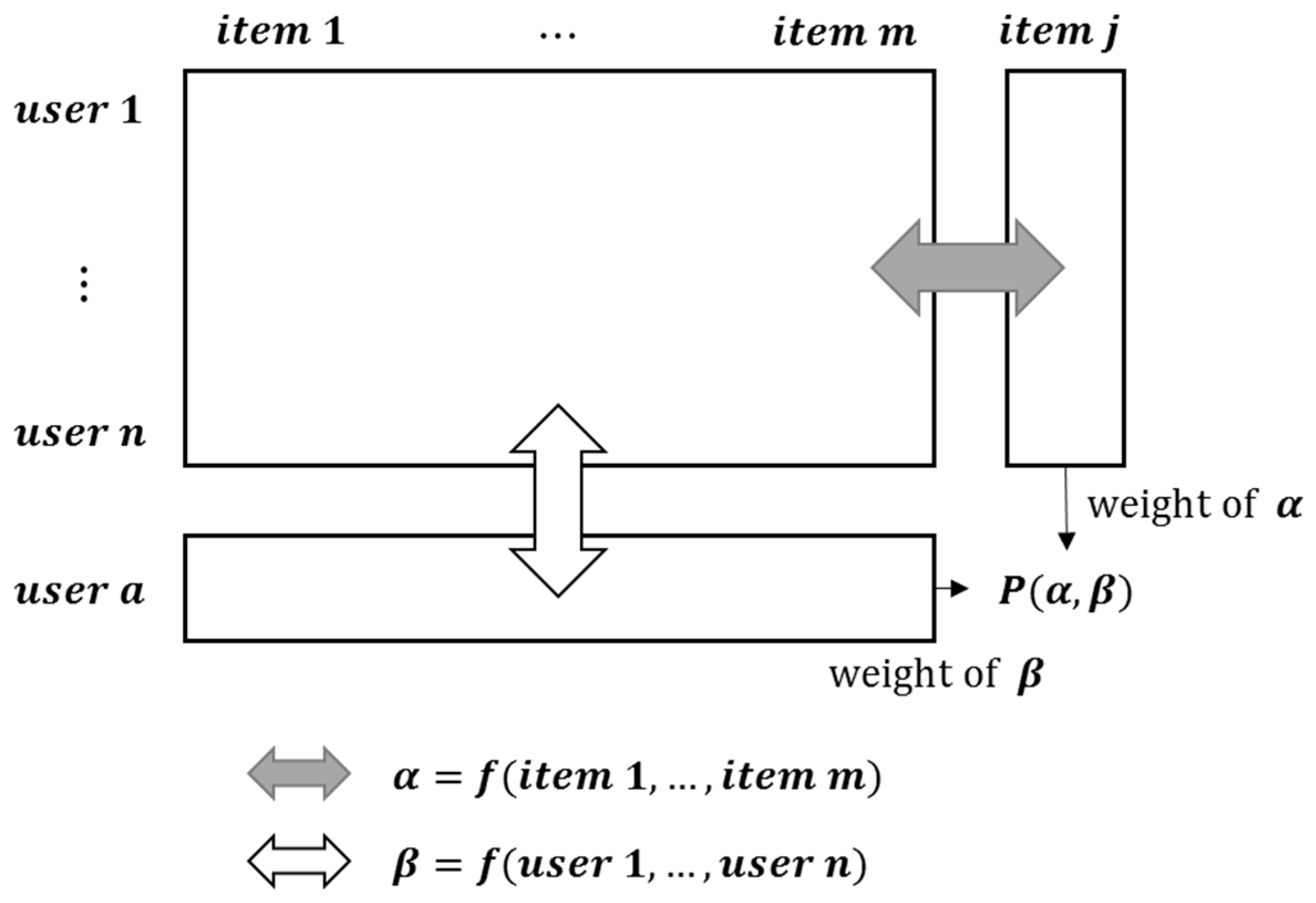
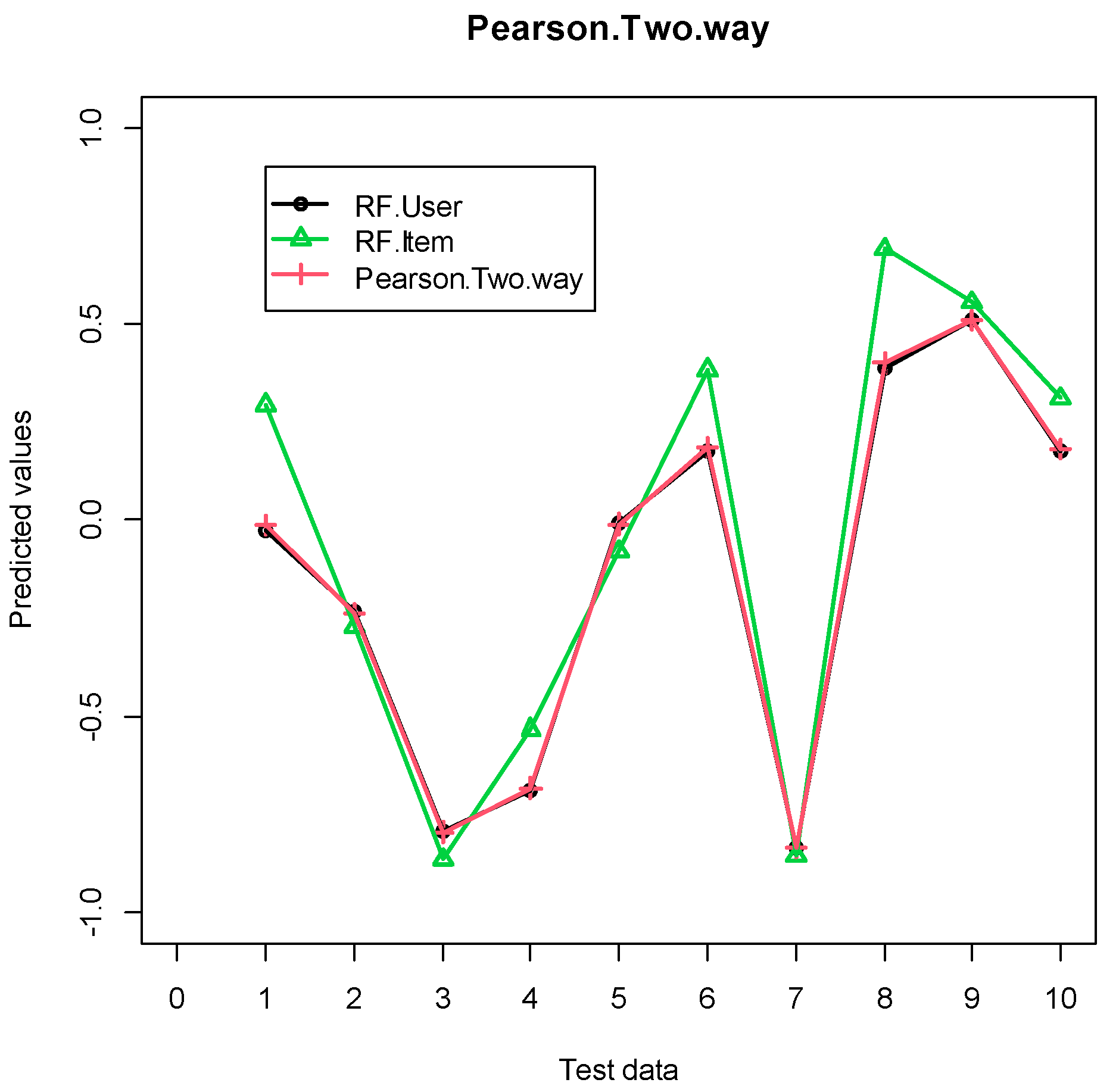
3.2. Pearson Correlation-Based Score

In (1) and (2), $k_a=1/{\displaystyle \sum }_{i=1}^n\left|w\left(a,i\right)\right|$ and $k_b=1/{\displaystyle \sum }_{j=1}^m\left|w\left(b,j\right)\right|$ are respectively multiplied to the sums of the correlations to consider the proportions of the contributions. Then, the Pearson correlation-based score for two-way cooperative CF is defined as a weighted mean of $P_{a{j}^{\prime }}$ and $P_{b{i}^{\prime }}$ as follows.

$$P_{P\left(P_{a{j}^{\prime }},P_{b{i}^{\prime }}\right)}=P_{a{j}^{\prime }}\frac{{{\displaystyle \sum }}_{i=1}^n\left|w\left(a,i\right)\right|}{{{\displaystyle \sum }}_{i=1}^n\left|w\left(a,i\right)\right|+{{\displaystyle \sum }}_{j=1}^m\left|w\left(b,j\right)\right|}+P_{b{i}^{\prime }}\frac{{{\displaystyle \sum }}_{j=1}^m\left|w\left(b,j\right)\right|}{{{\displaystyle \sum }}_{i=1}^n\left|w\left(a,i\right)\right|+{{\displaystyle \sum }}_{j=1}^m\left|w\left(b,j\right)\right|}$$

(8)

The first weight for $P_{a{j}^{\prime }}$, ${\displaystyle \sum }_{i=1}^n\left|w\left(a,i\right)\right|/({\displaystyle \sum }_{i=1}^n\left|w\left(a,i\right)\right|+{\displaystyle \sum }_{j=1}^m|w\left(b,j\right)|)$ is the proportion of the sum of the absolute values of the Pearson correlations between an active user $a$ and an existing user $i$, whereas the second weight for $P_{b{i}^{\prime }}$ ${\displaystyle \sum }_{j=1}^m\left|w\left(b,j\right)\right|/\left({\displaystyle \sum }_{i=1}^n\left|w\left(a,i\right)\right|+{\displaystyle \sum }_{j=1}^m\left|w\left(b,j\right)\right|\right)$ is the proportion of the sum of the absolute values of the Pearson correlations between an active item $b$ and an existing item $j$. Since the sum of the absolute values of the Pearson correlations reveals the importance of the prediction, the two proportions reasonably assign the importance of the prediction to the two predictions, $P_{a{j}^{\prime }}$ and $P_{b{i}^{\prime }}$.

For the extreme high-dimensional cold-start problem, where either the row of an active user or the column of an active item in the market basket data are all zeros, we propose that the corresponding Pearson correlations are considered as zeros because they cannot be calculated, and there are low correlations between the two variables. Then, the weighted mean can be reasonably calculated because both $P_{a{j}^{\prime }}$ and $P_{b{i}^{\prime }}$, the two predictions obtained by the user-based CF and by the item-based CF, become available.

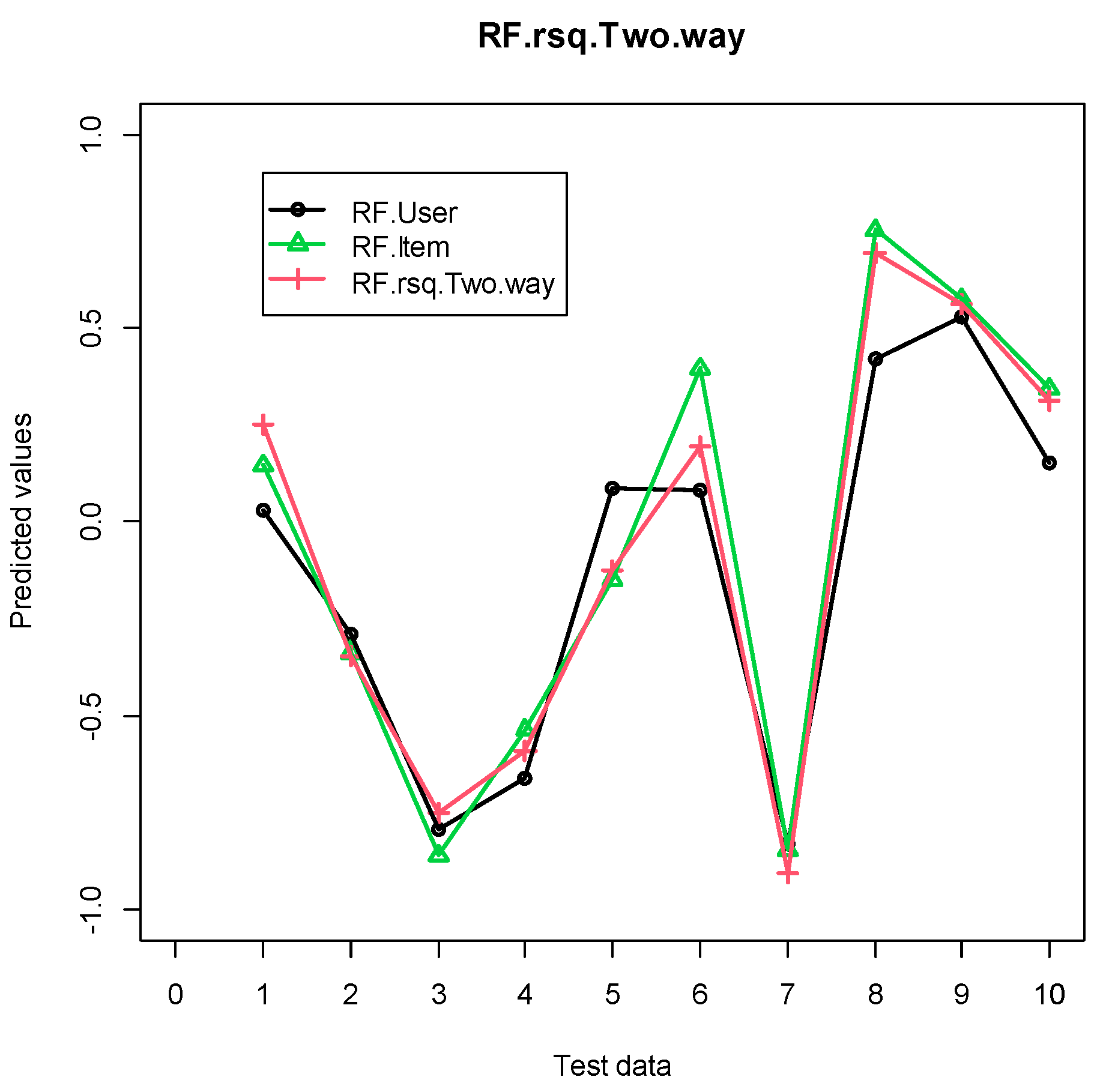
3.3. RF R-Square-Based Score and RF Pearson Correlation-Based Score

For the RF item modeling and the RF user modeling, we consider the average of the R-square (rsq) values of the RF regression approach to calculate a two-way cooperative score, because it represents a model adequacy. Based on (3) and (4), the RF R-square-based score is defined by

$$P_{rsq\left({\widehat{\mathit{v}}}_{\mathit{j}},{\widehat{\mathit{u}}}_{\mathit{i}}\right)}={\widehat{\mathit{v}}}_{\mathit{j}}\frac{({{\displaystyle \sum }}_{i=1}^{T_i}rs{q}_i)/T_i}{({{\displaystyle \sum }}_{i=1}^{T_i}rs{q}_i)/T_i+({{\displaystyle \sum }}_{j=1}^{T_j}rs{q}_j)/T_j}+{\widehat{\mathit{u}}}_{\mathit{i}}\frac{({{\displaystyle \sum }}_{j=1}^{T_j}rs{q}_j)/T_j}{({{\displaystyle \sum }}_{i=1}^{T_i}rs{q}_i)/T_i+({{\displaystyle \sum }}_{j=1}^{T_j}rs{q}_j)/T_j}$$

(9)

where $rs{q}_i$ is an R-square value of an $i$th regression tree for the RF item modeling; $rs{q}_j$ is an R-square value of a $j$th regression tree for the RF user modeling; $T_i$ is the number of regression trees for the item modeling; and $T_j$ is the number of regression trees for the user modeling. Since the average of R-square (rsq) values of the RF regression approach reveals the importance of the prediction, the two proportions reasonably assign the importance of the prediction to the two predictions, ${\widehat{\mathit{v}}}_{\mathit{j}}$ and ${\widehat{\mathit{u}}}_{\mathit{i}}$.

For the extreme high-dimensional cold-start problem, where either the row of an active user or the column of an active item in the binary market basket data are all zeros, the R-square values can have a negative sign when the mean squares of errors for the RF approach is greater than the variance of the response variable. Moreover, when the R package (randomForest) says that the R-square values are NaN, both the mean squares of errors for the RF approach and the variance of the response variable are zeros. Then, we consider the R-square values because the model fit is perfect. As a result, the weighted mean can be reasonably calculated. Additionally, instead of the average of R-square (rsq) values, we can adopt the proportion of the sum of the absolute values of the Pearson correlations for the voting scores, as follows, which is called an RF Pearson correlation-based score in this study.

$$P_{P\left({\widehat{\mathit{v}}}_{\mathit{j}}, {\widehat{\mathit{u}}}_{\mathit{i}}\right)}={\widehat{\mathit{v}}}_{\mathit{j}}\frac{{{\displaystyle \sum }}_{i=1}^n\left|w\left(a,i\right)\right|}{{{\displaystyle \sum }}_{i=1}^n\left|w\left(a,i\right)\right|+{{\displaystyle \sum }}_{j=1}^m\left|w\left(b,j\right)\right|}+{\widehat{\mathit{u}}}_{\mathit{i}}\frac{{{\displaystyle \sum }}_{j=1}^m\left|w\left(b,j\right)\right|}{{{\displaystyle \sum }}_{i=1}^n\left|w\left(a,i\right)\right|+{{\displaystyle \sum }}_{j=1}^m\left|w\left(b,j\right)\right|}$$

(10)

3.4. Scheme for RF R-Square-Based Score

For the extreme high-dimensional cold-start problem, the RF R-square-based score depends on an ad hoc approach considering even the inaccurately calculated average of the R-square (rsq) values. By leveraging on only the accurately calculated average of the R-square (rsq) values, we can improve the performance of the RF R-square-based score. We first consider both the average of the R-square values for the RF item modeling (item-rsq =$({\displaystyle \sum }_{i=1}^{T_i}rs{q}_i)/T_i$) and that for the RF user modeling (user-rsq =$({\displaystyle \sum }_{j=1}^{T_j}rs{q}_j)/T_j$) in (9). Indeed, we modify (9) according to the availabilities and the signs of item-rsq and user-rsq. The pseudocode of the proposed method is depicted below.

1. if (item-rsq != “NaN”) & (user-rsq != “NaN”)

  if (item-rsq > 0) & (user-rsq > 0)

$$P_{rsq\left({\widehat{\mathit{v}}}_{\mathit{j}}, {\widehat{\mathit{u}}}_{\mathit{i}}\right)}={\widehat{\mathit{v}}}_{\mathit{j}}\frac{({{\displaystyle \sum }}_{i=1}^{T_i}rs{q}_i)/T_i}{({{\displaystyle \sum }}_{i=1}^{T_i}rs{q}_i)/T_i+({{\displaystyle \sum }}_{j=1}^{T_j}rs{q}_j)/T_j}+{\widehat{\mathit{u}}}_{\mathit{i}}\frac{({{\displaystyle \sum }}_{j=1}^{T_j}rs{q}_j)/T_j}{({{\displaystyle \sum }}_{i=1}^{T_i}rs{q}_i)/T_i+({{\displaystyle \sum }}_{j=1}^{T_j}rs{q}_j)/T_j}$$

  else if (item-rsq < 0) & (user-rsq < 0)

$$P_{rsq\left({\widehat{\mathit{v}}}_{\mathit{j}}, {\widehat{\mathit{u}}}_{\mathit{i}}\right)}={\widehat{\mathit{v}}}_{\mathit{j}}\frac{({{\displaystyle \sum }}_{j=1}^{T_j}rs{q}_j)/T_j}{({{\displaystyle \sum }}_{i=1}^{T_i}rs{q}_i)/T_i+({{\displaystyle \sum }}_{j=1}^{T_j}rs{q}_j)/T_j}+{\widehat{\mathit{u}}}_{\mathit{i}}\frac{({{\displaystyle \sum }}_{i=1}^{T_i}rs{q}_i)/T_i}{({{\displaystyle \sum }}_{i=1}^{T_i}rs{q}_i)/T_i+({{\displaystyle \sum }}_{j=1}^{T_j}rs{q}_j)/T_j}$$

  else if (item-rsq > 0) & (user-rsq < 0) $P_{rsq\left({\widehat{\mathit{v}}}_{\mathit{j}}, {\widehat{\mathit{u}}}_{\mathit{i}}\right)}={\widehat{\mathit{v}}}_{\mathit{j}}$

  else if (item-rsq < 0) & (user-rsq > 0) $P_{rsq\left({\widehat{\mathit{v}}}_{\mathit{j}}, {\widehat{\mathit{u}}}_{\mathit{i}}\right)}={\widehat{\mathit{u}}}_{\mathit{i}}$

2. else if (item-rsq != “NaN”) & (user-rsq == “NaN”) $P_{rsq\left({\widehat{\mathit{v}}}_{\mathit{j}}, {\widehat{\mathit{u}}}_{\mathit{i}}\right)}={\widehat{\mathit{v}}}_{\mathit{j}}$

3. else if (item-rsq == “NaN”) & (user-rsq != “NaN”) $P_{rsq\left({\widehat{\mathit{v}}}_{\mathit{j}}, {\widehat{\mathit{u}}}_{\mathit{i}}\right)}={\widehat{\mathit{u}}}_{\mathit{i}}$

4. else if (item-rsq == “NaN”) & (user-rsq == “NaN”) $P_{rsq\left({\widehat{\mathit{v}}}_{\mathit{j}}, {\widehat{\mathit{u}}}_i\right)}=\mathbf{0}$

3.5. Computational Complexity Analysis

We usually analyze the computational complexity of recommender systems with consideration of two parts: computation time for model construction and that for one rating prediction. Based on a binary user-item matrix whose size is $n\times m$, the computational complexities of the user-based CF are $O\left(n^{2}mk\right)$ for model construction and $O\left(k\right)$ for one rating prediction. The former is to calculate similarities among users, and the latter is to make a prediction using $k$ neighbors. Likewise, the computational time of the item-based CF can estimated as $O\left(n{m}^{2}k\right)$ and $O\left(k\right)$. It is obvious that our approaches require more computational time for model construction because we employ the statistical learning algorithms. The computational complexities are $O\left(nm\right)$ for logistic regression and $O\left(\min \left(n^3,m^3\right)\right)$ for principal component analysis. The CART (classification and regression tree) algorithm has the complexity of $O\left(mn\log n\right)$ in the worst case, which means that the depth of a tree is $n$. If we build $s$ trees with $t$ randomly chosen variables at each split, the complexity of random forests becomes $O\left(stn\log n\right)$. Notice that the actual times for training prediction models can be reduced by performing PCA because we use a fewer number of input variables than $m$. Although our methods need more computational times for model construction than the existing CF approaches, their prediction complexity is $O\left(1\right)$, which means a constant time complexity because they do not use k neighbors. As a result of this small complexity for rating prediction, our methods are suitable for online recommendation, as other model-based approaches are. Our numerical experiments in the next section showed that the item-based CF took 0.05 s and our methods took 0.02 s for one rating prediction, although the PCA+LR item modeling and the RF item modeling took 5.29 s and 47.57 s respectively for model construction.

4. Numerical Experiments

4.1. Experimental Settings

Based on the experimental settings used by Mild and Reutterer [18] and Lee et al. [22], we consider both the Groceries dataset (arules R package) and the EachMovie dataset (https://grouplens.org/datasets/eachmovie/, accessed on 5 September 2004). For the Groceries dataset, 9835 transactions and 169 categories were collected for 30 days from a grocery store [25]. The first 20 existing users and 168 categories are selected, whereas the next 980 active users and 168 categories are selected. “Whole milk” is chosen as a new item. We consider classification error, recall, and precision for the predicted values, and actual values to evaluate the prediction performance.

The EachMovie dataset comprises 72,916 users and 1628 movies with 2,811,983 ratings, where a six-point scale with [0.0, 0.2, 0.4, 0.6, 0.8, 1.0] is considered. The ratings are converted into binary scales, and the experimental settings are used [22], where future responses or non-responses can be predicted for target marketing.

From the EachMovie dataset, 604 existing users and 207 movies (case 1), 150 existing users and 150 movies (case 2), 10 existing users and 100 movies (case 3), and 604 existing users and 20 movies (case 4) are randomly chosen for the section A $\times$ C in Figure 1a. Corresponding to the selected existing users and movies, 121 active users and 207 movies, 50 active users and 150 movies, 90 active users and 100 movies, and 121 active users and 20 movies are randomly selected for the section B $\times$ C in Figure 1a. Finally, 100 movies for new items (D in Figure 1a) are randomly chosen for 10 existing users and 100 movies, whereas 50 movies for new items (D in Figure 1a) are randomly chosen for the other cases. We consider Top-1, Top-2, …, and Top-10 accuracies as our performance measure [22]. For example, Top-10 accuracy is

$$\frac{\mathrm{The}\mathrm{number}\mathrm{of}\mathrm{the}\mathrm{actual}‘\text{Top-10}’\mathrm{items}}{\mathrm{The}\mathrm{number}\mathrm{of}\mathrm{first}\mathrm{ten}\mathrm{item}\mathrm{that}\mathrm{are}\mathrm{recommended}\mathrm{by}\mathrm{a}\mathrm{CF}\mathrm{scheme}}.$$

(11)

4.2. Experimental Results

4.2.1. Grocery Dataset

A cutoff value with a minimal classification error is chosen. For the best cutoff values,

Table 2. Prediction performance results.

	Classification Error	Precision	Recall	F1 Score
PCA+LR item modeling	$0.273\left(\frac{267}{980}\right)$	$0.475\left(\frac{28}{59}\right)$	$0.106\left(\frac{28}{264}\right)$	0.173
PCA+LR user modeling	$0.269\left(\frac{264}{980}\right)$	$0.500\left(\frac{18}{36}\right)$	$0.068\left(\frac{18}{264}\right)$	0.120
PCA+LR two-way 1	NA	NA	NA	NA
PCA+LR two-way 2	NA	NA	NA	NA
User-based CF	$0.267\left(\frac{262}{980}\right)$	$0.583\left(\frac{7}{12}\right)$	$0.026\left(\frac{7}{264}\right)$	0.050
Item-based CF	$0.261\left(\frac{256}{980}\right)$	$0.667\left(\frac{16}{24}\right)$	$0.060\left(\frac{16}{264}\right)$	0.110
Pearson correlation-based score	$0.260\left(\frac{255}{980}\right)$	$0.737\left(\frac{14}{19}\right)$	$0.053\left(\frac{14}{264}\right)$	0.099
RF item modeling	$0.260\left(\frac{255}{980}\right)$	$0.800\left(\frac{12}{15}\right)$	$0.046\left(\frac{12}{264}\right)$	0.087
RF user modeling	$0.260\left(\frac{255}{980}\right)$	$0.800\left(\frac{12}{15}\right)$	$0.046\left(\frac{12}{264}\right)$	0.087
RF R-square-based score	$0.261\left(\frac{256}{980}\right)$	$0.700\left(\frac{14}{20}\right)$	$0.053\left(\frac{14}{264}\right)$	0.099
RF Pearson correlation-based score	$0.259\left(\frac{254}{980}\right)$	$0.639\left(\frac{23}{36}\right)$	$0.087\left(\frac{23}{264}\right)$	0.153

presents the classification error, precision, recall, and F1 score of the CF approaches. As shown in Table 2, in terms of classification error, the RF Pearson correlation-based score is the best, whereas the RF item modeling and RF user modeling are the best in terms of precision. Regarding recall and F1 score, the PCA+LR item modeling works better than the other approaches, but its precision is the lowest.

Most significantly, the PCA+LR two-way 1 and PCA+LR two-way 2 fail to provide two-way predictions because of the high-dimensional cold-start problem. By contrast, the Pearson correlation-based score improves the classification error and precision of the user-based CF and item-based CF, whereas the RF Pearson correlation-based score improves the classification error, recall, and F1 score of the RF item modeling and RF user modeling. In conclusion, the two-way logistic regression approaches are outperformed by the proposed Pearson correlation-based score and RF Pearson correlation-based score.

4.2.2. Eachmovie Dataset

We calculate the Top-N accuracies for the approaches.

Table 3. Top-N accuracy for case 1.

N	PCA+LR User	PCA+LR Item	PCA+LR Two-Way 1	Pearson User	Pearson Item	Pearson Score	RF User	RF Item	RF rsq Score
1	0.926	0.926	0.917	0.893	0.843	0.884	0.926	0.934	0.934
2	0.905	0.921	0.917	0.868	0.855	0.872	0.921	0.917	0.913
3	0.909	0.917	0.912	0.862	0.857	0.871	0.917	0.904	0.909
4	0.899	0.907	0.899	0.847	0.855	0.853	0.897	0.895	0.903
5	0.891	0.893	0.891	0.812	0.833	0.823	0.873	0.881	0.893
6	0.858	0.855	0.854	0.788	0.807	0.803	0.850	0.864	0.869
7	0.837	0.832	0.835	0.769	0.782	0.775	0.829	0.836	0.837
8	0.807	0.802	0.808	0.738	0.754	0.750	0.813	0.813	0.817
9	0.778	0.775	0.786	0.717	0.731	0.731	0.778	0.789	0.793
10	0.751	0.752	0.757	0.704	0.696	0.711	0.754	0.759	0.771
Avg.	0.856	0.858	0.858	0.800	0.801	0.807	0.856	0.859	0.864

summarizes the Top-N accuracy for case 1, where we can effectively check the recommendation performance by manipulating the N. The Top-N accuracy ranging from 0 to 1 has been widely used for evaluating the recommendation performance because the N can be selected by recommender system managers, and they are interested in how many items among the recommended ones would be actually chosen by users [18,19,20,21,22,23,24]. The bold numbers in the table indicate the best performances. In case 1, for the PCA+LR item modeling and PCA+LR user modeling, the PCA+LR two-way 1 performs the best for Top-8, Top-9, and Top-10, whereas the PCA+LR user modeling is the best for Top-1, Top-6, and Top-7, and the PCA+LR item modeling is the best for Top-1 to Top-5. For the user-based CF and item-based CF, the Pearson correlation-based score performs the best for Top-2, Top-3, Top-9, and Top-10, whereas the user-based CF performs the best for Top-1 and the item-based CF does for Top-4 to Top-9. For the RF item modeling and RF user modeling, the RF R-square-based score performs the best for Top-1 and Top-4 to Top-10, whereas the RF user modeling performs the best for Top-3 and the RF item modeling does for Top-1 and Top-2. For the two-way cooperative CF, the Pearson correlation-based score and the RF R-square-based score provide the best average of the ten Top-N accuracies. Therefore, we realize that the Pearson correlation-based score as well as the RF R-square-based score works more effectively than the PCA+LR two-way 1. Note that there are 604 users and 207 items in section A $\times$ C in Figure 1a.

In case 2, as shown in

Table 4. Top-N accuracy for case 2.

N	PCA+LR User	PCA+LR Item	PCA+LR Two-Way 1	Pearson User	Pearson ITEM	Pearson Score	RF User	RF Item	RF rsq Score
1	0.940	0.940	0.920	0.880	0.780	0.920	0.900	0.920	0.920
2	0.900	0.880	0.910	0.870	0.790	0.870	0.850	0.900	0.900
3	0.867	0.860	0.860	0.873	0.727	0.873	0.867	0.893	0.893
4	0.860	0.855	0.850	0.875	0.730	0.875	0.820	0.860	0.865
5	0.840	0.828	0.844	0.832	0.708	0.840	0.800	0.836	0.836
6	0.803	0.793	0.797	0.777	0.683	0.790	0.770	0.800	0.800
7	0.766	0.746	0.754	0.740	0.660	0.740	0.734	0.763	0.777
8	0.735	0.705	0.715	0.705	0.633	0.710	0.703	0.725	0.743
9	0.691	0.678	0.693	0.689	0.611	0.687	0.678	0.696	0.708
10	0.660	0.662	0.672	0.670	0.592	0.664	0.654	0.684	0.674
Avg.	0.806	0.795	0.802	0.791	0.691	0.797	0.778	0.808	0.812

, for the PCA+LR item modeling and PCA+LR user modeling, the PCA+LR two-way 1 performs the best for Top-2, Top-3, Top-9, and Top-10, whereas the PCA+LR user modeling is the best for Top-1 and Top-4 toTop-8 and the PCA+LR item modeling is the best for Top-1.

For the user-based CF and item-based CF, the Pearson correlation-based score performs the best for Top-1 to Top-8, whereas the user-based CF performs the best for Top-2 to Top-4, Top-7, Top-9, and Top-10; the item-based CF is outperformed by the two approaches. The RF R-square-based score performs the best for Top-1 to Top-9, whereas the RF item modeling performs the best for Top-1 to Top-3, Top-5, Top-6, and Top-10; the RF user modeling is outperformed by the two approaches. For the two-way cooperative CF, the Pearson correlation-based score and the RF R-square-based score provide the best average of the ten Top-N accuracies.

Therefore, we assume that both the Pearson correlation-based score and the RF R-square-based score work very effectively for the two-way cooperative CF than the PCA+LR two-way 1. Note that there are 150 users and 150 items in section A $\times$ C in Figure 1a.

In case 3, as shown in

Table 5. Top-N accuracy for case 3.

N	PCA+LR User	PCA+LR Item	PCA+LR 2-Way 1	PCA+LR 2-Way 2	Pearson User	Pearson Item	Pearson Score	RF User	RF Item	RF rsq Score	RF Pearson Score
1	0.49	0.67	0.49	0.54	0.71	0.41	0.30	0.66	0.63	0.57	0.79
2	0.47	0.66	0.40	0.48	0.73	0.38	0.24	0.71	0.71	0.59	0.71
3	0.42	0.62	0.37	0.44	0.68	0.39	0.27	0.66	0.65	0.56	0.65
4	0.43	0.56	0.38	0.45	0.63	0.38	0.26	0.61	0.61	0.53	0.62
5	0.42	0.55	0.36	0.42	0.60	0.37	0.24	0.58	0.58	0.53	0.60
6	0.42	0.53	0.35	0.42	0.56	0.36	0.23	0.57	0.56	0.53	0.57
7	0.44	0.52	0.36	0.44	0.54	0.35	0.25	0.54	0.54	0.50	0.54
8	0.43	0.50	0.35	0.43	0.51	0.34	0.23	0.52	0.52	0.49	0.53
9	0.42	0.49	0.34	0.42	0.50	0.34	0.23	0.49	0.50	0.48	0.52
10	0.41	0.47	0.34	0.41	0.49	0.33	0.23	0.48	0.47	0.47	0.50
Avg.	0.44	0.56	0.37	0.45	0.60	0.36	0.25	0.58	0.58	0.53	0.60

, the PCA+LR item modeling performs better than the other approaches for all the Top-N accuracies. The PCA+LR two-way 2 seems not to outperform the PCA+LR user modeling, although it clearly outperforms the PCA+LR two-way 1. For the user-based CF and item-based CF, the Pearson correlation-based score and the item-based CF are outperformed by the user-based CF for all the Top-N accuracies. The Pearson correlation-based score does not seem to work well. The RF R-square-based score is outperformed by the RF user modeling and the RF item modeling.

Note that there are only 10 users in section A $\times$ C in Figure 1a. In this case, the columns of some active items in the market basket data are all zeros, which is the extreme high-dimensional cold-start problem. Then, the average of the R-square values can have a negative sign, which can lead to bad prediction performance.

For instance, we randomly select a test observation where 1 denotes a purchased item and −1 denotes a non-purchased item where the predicted values of the item modeling and the user modeling range from −1 to 1. The predicted value of the item modeling is −0.3204994, and the predicted value of the user modeling is −0.5009333. The average of the R-square values of the item modeling is 0.251122 and the average of the R-square values of the user modeling is −0.3145476, which has a negative sign. Then, the calculated weighted average based on (9) is −1.215328, which does not make sense because it does not fall between −0.3204994 and 0.5009333. Therefore, the RF R-square-based score does not work well in this case.

Instead of the RF R-square-based score, we apply the Pearson correlation-based score to the RF item and user modeling. For Top-1 and Top-4 to Top-6, the RF Pearson correlation-based score performs the best and is close to the RF user modeling or the RF item modeling for the other Top-N accuracies. Moreover, the RF Pearson correlation-based score gives the best average of the ten Top-N accuracies. As a result, we realize that the RF Pearson correlation-based score works better for the two-way cooperative CF than the RF R-square-based score.

For case 4, as shown in

Table 6. Top-N accuracy for case 4.

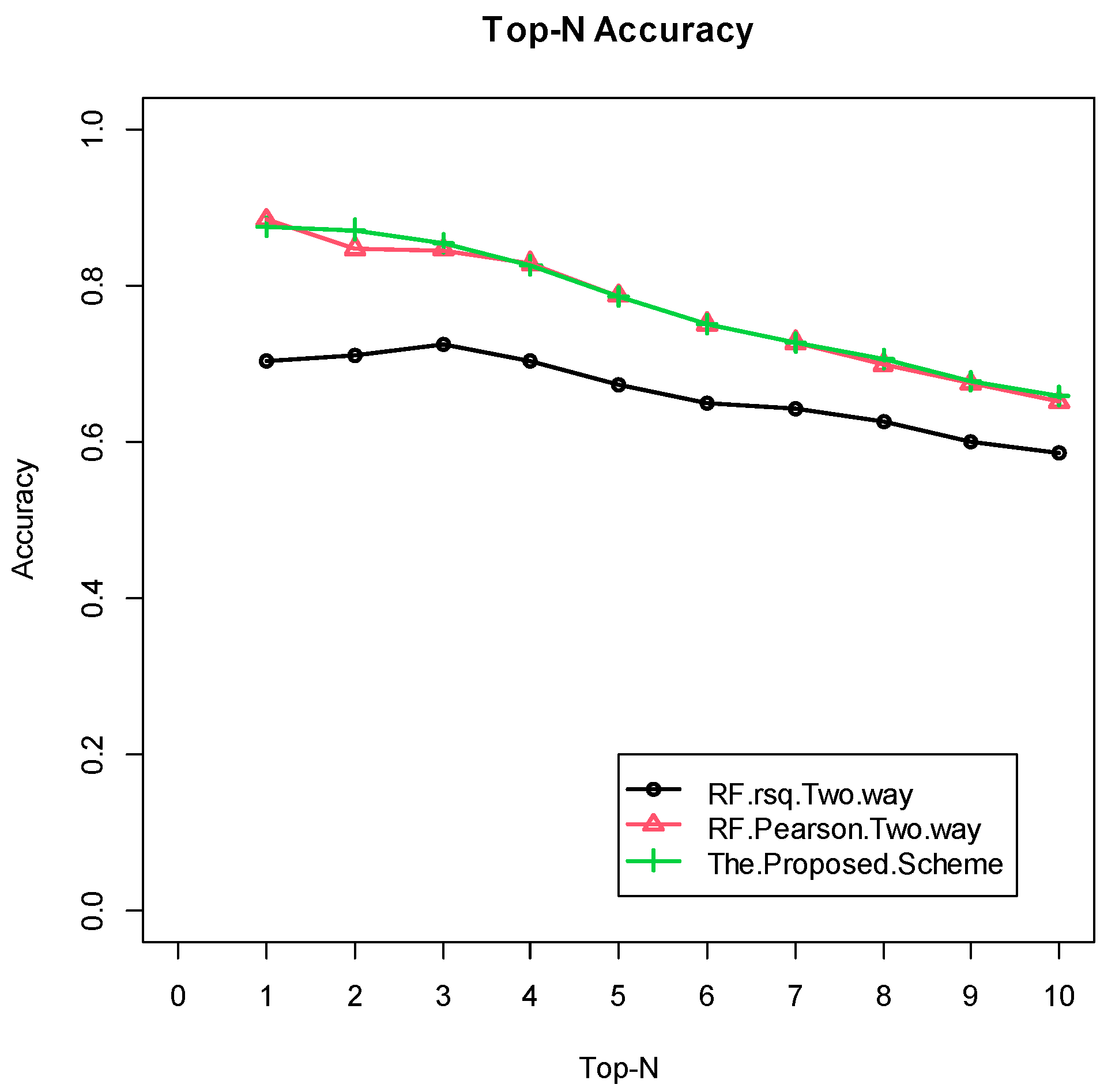
N	PCA +LR User	PCA +LR Item	PCA +LR 2-Way 1	PCA +LR 2-Way 2	Pearson User	Pearson Item	Pearson Score	RF User	RF Item	RF rsq 2-Way	RF Pearson Score
1	0.76	0.87	NA	0.69	0.84	0.68	0.85	0.86	0.88	0.70	0.88
2	0.73	0.87	NA	0.74	0.84	0.63	0.83	0.84	0.86	0.71	0.85
3	0.71	0.85	NA	0.74	0.82	0.62	0.82	0.83	0.84	0.73	0.85
4	0.67	0.84	NA	0.74	0.81	0.62	0.80	0.81	0.81	0.70	0.83
5	0.64	0.82	NA	0.71	0.77	0.62	0.77	0.76	0.79	0.67	0.79
6	0.61	0.78	NA	0.69	0.75	0.61	0.74	0.74	0.76	0.65	0.75
7	0.59	0.75	NA	0.67	0.71	0.59	0.71	0.70	0.73	0.64	0.73
8	0.57	0.71	NA	0.64	0.68	0.57	0.68	0.68	0.70	0.63	0.70
9	0.56	0.69	NA	0.62	0.66	0.56	0.66	0.65	0.68	0.60	0.68
10	0.55	0.67	NA	0.61	0.64	0.54	0.64	0.63	0.65	0.59	0.65
Avg.	0.64	0.79	NA	0.69	0.75	0.60	0.75	0.75	0.77	0.66	0.77

, the PCA+LR item modeling performs better than the other approaches for all the Top-N accuracies. The PCA+LR two-way 2 does not seem to outperform the PCA+LR item modeling, although it clearly outperforms the PCA+LR two-way 1. The PCA+LR two-way 1 does not even provide appropriate predicted values. For the user-based CF and item-based CF, the user-based CF and the Pearson correlation-based score outperform the item-based CF for all the Top-N accuracies. The Pearson correlation-based score does not seem to perform the best, except for Top-1 and Top-8. The RF R-square-based score is outperformed by the RF user modeling and the RF item modeling. Note that there are only 20 items in section $\mathrm{A}\times$ C in Figure 1a. In this case, the rows of some active users in the binary market basket data are all zeros, which is the extreme high-dimensional cold-start problem. Then, the average of the R-square values can have a negative sign, which can lead to bad prediction performance.

For further analysis, we randomly select 10 test data and respectively calculate predicted values for the RF user modeling, the RF item modeling, and the RF R-square-based score, as shown in Figure 3, where 1 denotes a purchased item and −1 denotes a non-purchased item. Although the RF R-square-based score is a weighted average of the RF item modeling-based prediction and the RF user modeling-based prediction, the first, second, third, and seventh observations violate the assumption that the weighted mean should fall between the predicted value of the RF item modeling and the predicted value of the RF user modeling, as illustrated in Figure 3, because the averages of the R-square values have negative signs. As a result, the RF R-square-based score does not work well.

Instead, we apply the Pearson correlation-based score to the RF item modeling and the RF user modeling. For Top-1, Top-3, Top-4, and Top-10, the RF Pearson correlation-based score performs the best and is close to the item modeling for the other Top-N accuracies, as shown in Table 6. Moreover, the RF Pearson correlation-based score gives the best average of the ten Top-N accuracies. Thus, the RF Pearson correlation-based score works better for the two-way cooperative CF than the RF R-square-based score. To understand these matters better, we randomly select 10 test data and calculate predicted values for the RF user modeling, the RF item modeling, and the RF Pearson correlation-based score (Figure 4), where 1 denotes a response and −1 denotes a non-response. The RF Pearson correlation-based score should be a weighted average of the RF item modeling-based prediction and the RF user modeling-based prediction. In this case, no observations violate the assumption. In other words, the RF Pearson correlation-based scores always fall between the predicted value of the RF item modeling and the RF predicted value of the user modeling. Thus, the RF Pearson correlation-based score works more effectively than the RF R-square-based score for the two-way cooperative CF.

Additionally, although the proposed CF scheme for the RF R-square-based score in Section 3 D requires more procedures, it improves the prediction performance of the RF R-square-based score dramatically, as shown in Table 6. As illustrated in Figure 5, the proposed CF scheme emulates the RF Pearson correlation-based score. Indeed, the average of the ten Top-N accuracies for the proposed CF scheme, 0.7737, is greater than that of the ten Top-N accuracies for the Pearson correlation-based score, 0.7696. We realize that the proposed CF scheme performs as well as the RF Pearson correlation-based score for the two-way cooperative CF.

5. Conclusions

In this study, we propose a PCA+LR two-way 2, a Pearson correlation-based score, an RF R-square-based score, an RF Pearson correlation-based score, and a CF scheme for the RF R-square-based score for two-way cooperative CF for binary market basket data. The experimental results show that the proposed two-way cooperative CF approaches work better than the existing PCA+LR two-way 1. For the Grocery dataset, the PCA+LR two-way 1 does not even provide an appropriate predicted value, which demonstrates that it is clearly outperformed by the Pearson correlation-based score and RF Pearson correlation-based score. For the non-high-dimensional EachMovie dataset, the Pearson correlation-based score as well as the RF R-square-based score clearly improve the accuracy of the one-way approaches, whereas the PCA+LR two-way 1 does not. For the extreme high-dimensional EachMovie dataset, only the RF Pearson correlation-based score and the proposed CF scheme clearly improve the performance of the one-way approaches.

Most significantly, for the first time, we apply the proposed two-way cooperative CF approaches to the Grocery transaction dataset and obtain promising results. Two-way cooperative CF is crucial for binary market basket data; therefore, the proposed two-way cooperative CF approaches would be useful for marketing practitioners. However, the two proposed CF approaches cannot always improve the performance of the one-way CF approaches because the prediction performance depends on the datasets. In our future research, we plan to apply the proposed two-way CF approaches to other domains and employ other supervised learning approaches.

References

- Su, X.; Khoshgoftaar, T.M. A Survey of Collaborative Filtering Techniques. Adv. Artif. Intell. 2009, 2009, 421425. [Google Scholar] [CrossRef]
- Park, D.H.; Kim, H.K.; Choi, I.Y.; Kim, J.K. A research. Expert Syst. Appl. 2012, 39, 10059–10072. [Google Scholar] [CrossRef]
- Ahn, H.J. A new similarity measure for collaborative filtering to alleviate the new user cold-starting problem. Inf. Sci. 2008, 178, 37–51. [Google Scholar] [CrossRef]
- Schein, A.; Popescul, A.; Ungar, L.H. Methods and metrics for cold-start recommendations. In Proceedings of the 25th Annual International ACM SIGIR Conference on Research and Development in Information Retrieval, Tampere, Finland, 11–15 August 2002; pp. 253–260. [Google Scholar]
- Park, S.T.; Chu, W. Pairwise preference regression for cold-start recommendation. In Proceedings of the third ACM Conference on Recommender Systems (RecSys2009), New York, NY, USA, 22–25 October 2009; pp. 21–28. [Google Scholar]
- Chen, C.C.; Wan, Y.-H.; Chung, M.-C.; Sun, Y.-C. An effective recommendation method for cold start new users using trust and distrust networks. Inf. Sci. 2013, 224, 19–36. [Google Scholar] [CrossRef]
- Lika, B.; Kolomvatsos, K.; Hadjiefthymiades, S. Facing the cold start problem in recommender systems. Expert Syst. Appl. 2013, 41, 2065–2073. [Google Scholar] [CrossRef]
- Liu, H.; Hu, Z.; Mian, A.; Tian, H.; Zhu, X. A new user similarity model to improve the accuracy of collaborative filtering. Knowl. -Based Syst. 2014, 56, 156–166. [Google Scholar] [CrossRef] [Green Version]
- Son, L.H. Dealing with the new user cold-start problem in recommender systems: A comparative review. Inf. Syst. 2016, 58, 87–104. [Google Scholar] [CrossRef]
- JBreese, S.; Heckerman, D.; Kadie, C. Empirical Analysis of Predictive Algorithms for Collaborative Filtering; Technical Report MSR-TR-98-12; Microsoft Research: Redmond, WA, USA, 1998. [Google Scholar]
- Choi, K.; Suh, Y. A new similarity function for selecting neighbors for each target item in collaborative filtering. Knowl.-Based Syst. 2013, 37, 146–153. [Google Scholar] [CrossRef]
- Goldberg, D.; Nichols, D.; Oki, B.M.; Terry, D. Using collaborative filtering to weave an information tapestry. Commun. ACM 1992, 35, 61–70. [Google Scholar] [CrossRef]
- Leung, C.W.-K.; Chan, S.C.-F.; Chung, F.-L. An empirical study of a cross-level association rule mining approach to cold-start recommendations. Knowl.-Based Syst. 2008, 21, 515–529. [Google Scholar] [CrossRef]
- Tsai, C.-F.; Hung, C. Cluster ensembles in collaborative filtering recommendation. Appl. Soft Comput. 2011, 12, 1417–1425. [Google Scholar] [CrossRef]
- Stai, E.; Kafetzoglou, S.; Tsiropoulou, E.E.; Papavassiliou, S. A holistic approach for personalization, relevance feedback & recommendation in enriched multimedia content. Multimed. Tools Appl. 2018, 77, 283–326. [Google Scholar]
- Burke, R. Hybrid Recommender Systems: Survey and Experiments. User Model. User-Adapt. Interact. 2002, 12, 331–370. [Google Scholar] [CrossRef]
- Thai, M.T.; Wu, W.; Xiong, H. Big Data in Complex and Social Networks; CRC Press: Boca Raton, FL, USA, 2016. [Google Scholar]
- Mild, A.; Reutterer, T. An improved collaborative filtering approach for predicting cross-category purchases based on binary market basket data. J. Retail. Consum. Serv. 2003, 10, 123–133. [Google Scholar] [CrossRef] [Green Version]
- Mild, A.; Reutterer, T. Collaborative Filtering Methods for Binary Market Basket Data Analysis. In International Computer Science Conference on Active Media Technology; Springer: Berlin/Heidelberg, Germany, 2001; Volume 2252, pp. 302–313. [Google Scholar] [CrossRef]
- Hwang, W.Y. Variable Selection for Collaborative Filtering with the Market Basket Data. Int. Trans. Oper. Res. 2020, 27, 3167–3177. [Google Scholar] [CrossRef]
- Hwang, W.-Y. Assessing new correlation-based collaborative filtering approaches for binary market basket data. Electron. Commer. Res. Appl. 2018, 29, 12–18. [Google Scholar] [CrossRef]
- Lee, J.; Jun, C.-H.; Kim, S. Classification-based collaborative filtering using market basket data. Expert Syst. Appl. 2005, 29, 700–704. [Google Scholar] [CrossRef]
- Hwang, W.-Y.; Jun, C.-H. Supervised Learning-Based Collaborative Filtering Using Market Basket Data for the Cold-Start Problem. Ind. Eng. Manag. Syst. 2014, 13, 421–431. [Google Scholar] [CrossRef] [Green Version]
- Lee, J.-S.; Olafsson, S. Two-way cooperative prediction for collaborative filtering recommendations. Expert Syst. Appl. 2009, 36, 5353–5361. [Google Scholar] [CrossRef]
- Hahsler, M.; Hornik, K.; Reutterer, T. Implications of Probabilistic Data Modeling for Mining Association Rules. In From Data and Information Analysis to Knowledge Engineering; Springer: Berlin/Heidelberg, Germany, 2006; pp. 598–605. [Google Scholar]