Abstract
When the CNC machining of continuous small line segments is performed, the direction of the machine tool movement will change abruptly at the corner of adjacent line segments. Therefore, a reasonable constraint on the feedrate at the corner is the prerequisite for achieving high-speed and high-precision machining. To achieve this goal, a feedrate-constraint method based on the nominal acceleration was proposed. The proposed method obtains the predicted value of acceleration during the machining process by the machining trajectory prediction and acceleration filtering. Then, the feedrate at the corner is constrained, according to the predicted acceleration. Specifically, for any corner of adjacent line segments, the proposed method assumes that the CNC machining of a short path centered on the corner is carried out at a constant feedrate. First, the actual machining trajectory is predicted according to the transfer function of the servo system. Then, the nominal acceleration, when the CNC machining is carried out to the corner, is calculated and processed by a low-pass FIR filter. Last, the feedrate-constraint value at the corner is obtained according to the nominal acceleration and the preset normal acceleration. The advantage of the proposed method is that it can be used for different machining paths consisting of long segments or continuous small segments and it has no special requirement for the accuracy of the machining path. As a result, the feedrate-constraint value obtained is reasonable and the smooth machining process can be ensured. The simulation results in both 2D and 3D machining paths show that the proposed method is insensitive to the length of the line segment and the angle of the corner, and the calculated feedrate-constraint value is close to the theoretical value, which has good stability and versatility. In contrast, the feedrate-constraint values obtained by conventional methods change abruptly along the machining path, especially in the 3D simulation, which will damage the machining quality. The experiment was performed on a three-axis CNC machine tool controlled by a self-developed controller, and a free-form surface workpiece was machined by a conventional feedrate-constraint method and the proposed method, respectively. The experimental results showed that the proposed method can make the feedrate of the machining process higher and more stable. Then, machining defects such as overcutting and undercutting can be avoided and the machining quality can be improved. Therefore, the article proposes a new method to constrain the feedrate at the corner of continuous small line segments, which can improve the machining efficiency and quality of the CNC machining.
1. Introduction
The continuous small line segments are widely used in CNC machining [1,2,3], which are universal and easy to calculate. However, the direction of the machining movement will change abruptly at corners of adjacent line segments, which brings many difficulties to the realization of precise and efficient CNC machining [4,5,6]. One significant difficulty is to constrain the feedrate reasonably at corners [7,8]. Too low a feedrate at the corner will increase the machining time, while too high will cause the machine tool to vibrate and damage the machining quality.
A reasonable constraint on the feedrate at the corner of continuous small line segments is very important for achieving high-speed and high-precision machining. Two commonly used constraint methods are the angle-constraint method and the curvature-constraint method. The angle-constraint method first calculates the angle of the corner of adjacent line segments and then substitutes it into a mathematical model to obtain the corresponding feedrate-constraint value. As in the literature [9,10], scholars assume that the magnitude of the velocity (a vector) of the machine tool remains constant during machining a corner and that the change of the velocity direction is completed within one interpolation cycle, which generates a steering acceleration during the process. Then, according to the relationship among the steering acceleration, the angle, and the velocity magnitude, the feedrate-constraint value can be achieved from the angle, under the constraint that the steering acceleration does not exceed the preset upper limit. The literature [11] assumes that there exists a virtual transition arc at the corner. Firstly, the radius of the arc is obtained according to the corner’s angle and the maximum allowable value of transition error. Then, the feedrate-constraint value of the transition arc is calculated according to the radius and the preset upper limit of the normal acceleration, which will be used as the feedrate-constraint value at the corner. In the literature [12], considering that the length of each line segment is usually not exactly the sum of integer interpolation cycles, the interpolation across line segments at the corner will cause the trajectory error in machining. According to the relationship among the trajectory error, the corner’s angle, and the feedrate, the feedrate-constraint value can be obtained from the angle under the constraint that the trajectory error does not exceed the preset upper limit. The angle-constraint method above has good performance for the area with long line segments in the machining path (hereafter referred to as “Line Area”), but for the continuous small line segments discretized from the curve (hereafter referred to as “Curve Area”), the calculated angle will be small and unstable due to the short line segments, which will eventually cause the feedrate-constraint value to be overlarge and unstable.
The curvature-constraint method first calculates the radius of curvature of the continuous small line segments and then obtains the feedrate-constraint value based on the radius of curvature. For example, the Syntec CNC [13] uses a virtual arc to approach the path of two adjacent line segments and calculates the chord error. If the chord error is small enough, the line segments will be recognized as Curve Area and its radius of curvature will be calculated. Similarly, the literature [14] estimates the radius of curvature corresponding to the current corner based on the geometric information of several adjacent small line segments around this corner, while the literature [15] first groups small line segments by the length of the line segment and the angle of the corner and then calculates the radius of curvature corresponding to each group. After that, the feedrate-constraint value can be obtained from the radius of curvature and the preset upper limit of normal acceleration. For Curve Area in the machining path, the above curvature-constraint method can achieve good results, but since curvature is a unique property of curves, the feedrate-constraint value obtained by this method is not reasonable for Line Area.
In addition, some scholars obtain the feedrate-constraint value for continuous small line segments based on the limitations of acceleration of each axis [16,17,18] or contour error [19], but the calculation result will be unstable when the length of the line segment is too short. In recent years, some other scholars inserted a transition curve such as PH [20] and B-Spline [21,22,23] at the corner of adjacent line segments. Then, the feedrate can be constrained according to the curvature of the transition curve. At the same time, the machining path will be smoother. However, if the line segment is too short, the transition curve will be hard to insert. Fitting continuous small line segments to a curve such as Akima [24], B-Spline [25], and NURBS [26,27] is another similar method, and the method is also used by Siemens 840D CNC [28]. However, the trajectory error between the fitting curve and the original line segments is inevitable, which will damage machining quality. Additionally, there are many difficulties [29] in the feedrate planning and interpolation of the transition and fitting curve.
To address the above problems, this paper proposes a Feedrate-constraint method for the continuous small line segments based on the Nominal Acceleration (FNA). The FNA method obtains the predicted value of acceleration during machining process by the machining trajectory prediction and acceleration filtering, and the feedrate of the actual machining process is constrained according to the predicted acceleration. Compared with conventional methods, the FNA method is not sensitive to the angle of the corner and the length of the line segment, so it can be used for different machining paths consisting of long segments or continuous small segments, and it has no special requirements for the accuracy of the machining path. Therefore, the feedrate-constraint value obtained by this method is more reasonable and stable, which can improve the quality and efficiency of the CNC machining. In the following section, the FNA method will be introduced in detail and its effectiveness will be verified by simulation and experiment. This paper is organized as follows: Section 2 is the introduction of the FNA method; Section 3 is the simulation and experiment; and Section 4 is the conclusion.
2. The FNA Method
The principle of the FNA method proposed in this paper is as follows. For a certain corner in the machining path, whose feedrate-constraint value needs to be solved, assume that a constant feedrate is used for the CNC machining of the small line segments around this corner. Predict the actual machining trajectory based on the numerical analysis method of discrete systems. Then, obtain the predicted value of acceleration when the machining is carried out to the corner. Finally, calculate the feedrate-constraint value according to the predicted value of acceleration and its maximum allowable value.
Specifically, for a certain corner of adjacent line segments whose feedrate-constraint value is to be solved, the whole process of the FNA method is shown in Figure 1, including (1) parsing the ISO6983 code and recording the endpoints of each line segment; (2) sampling the small line segments in the sampling interval containing the point in Figure 1a to generate a position sampling sequence ; (3) predicting the corresponding machining trajectory of after the servo system, so as to generate the position sequence , which is closer to the actual machining trajectory; (4) using the difference method to obtain the corresponding acceleration sequence from , and then using a FIR low-pass filter to process , so as to obtain the nominal acceleration corresponding to the sampling interval; and (5) obtaining the feedrate-constraint value according to and the preset upper limit of normal acceleration . The main parts of the above process will be discussed in detail below.
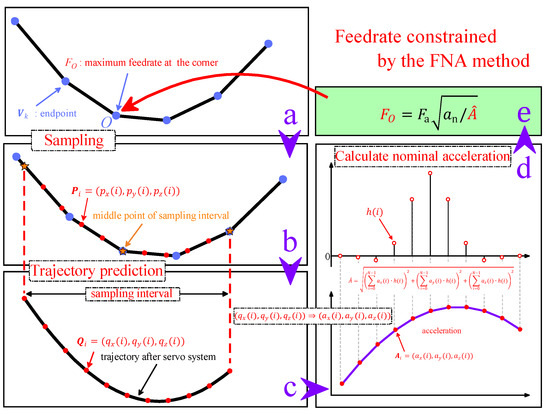
Figure 1.
Flowchart of the FNA method.
2.1. The Generation of Position Sampling Sequence
In the flow of the FNA method shown in Figure 1, the machining trajectory predicting, the acceleration filtering, and the nominal acceleration solving, is based on discrete digital signals. Therefore, it is necessary to sample the continuous small line segments to generate a discrete position sampling sequence. The sampling process mainly consists of two steps: (1) Starting from the point , the small line segments are traversed in the backward/forward direction, respectively, until the traversed distance reaches the preset target value and ; and (2) the traversed region of the machining path is taken as the sampling interval, and points are sampled along the small line segments in this interval, thus generating the position sampling sequence :
In Figure 1, the sampling interval of each part of the FNA method is a symmetric interval with point as the midpoint for easy understanding, but, in fact, the sampling intervals of these parts are not the same and not all of them are symmetric, which depends on the specific needs of each part.
2.2. The Prediction of Machining Trajectory
The position sequence shown in Equation (1) has been achieved according to the previous section. However, due to the trajectory characteristics of the small line segments and the position error [30], will inevitably contain a random position error , which, in turn, causes fluctuations in the velocity and acceleration as
where is the sampling period. If and are taken to be and , respectively, the acceleration fluctuation will be as high as .
On the other hand, in the actual CNC machining process, will be transmitted to the servo system to control the motion of the machine tool. Since the output of the servo system will lag behind the input [31], there will be a difference between the actual machining trajectory and the command trajectory, which, in turn, will lead to a change in the corresponding speed and acceleration.
For the above two reasons, this section will use the analysis method of the discrete system to predict the “actual machining trajectory” corresponding to , and the solving of the nominal acceleration in a later section will be based on to make the final feedrate-constraint value be more reasonable.
The function and control structure of the servo system of a typical three-axis CNC machine tool is shown in Figure 2, in which and are the transfer functions of each axis. In order to solve the position sequence of the servo system output, the difference equation corresponding to the transfer function of each axis should be obtained first, and then the command position sequence can be substituted into it to calculate . Since the servo system of each axis usually has the same control structure, take the X-axis as an example and let its input and output position sequences be and , respectively. Then, when is approximated as a second-order system [32,33], its corresponding difference equation is
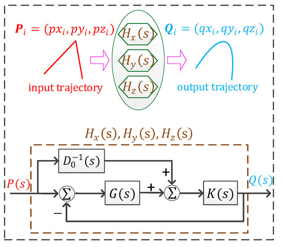
Figure 2.
The function and control structure of the servo system.
The solution of the coefficients and initial conditions of this difference equation will be detailed below.
2.2.1. The Solution of Difference Equation Coefficients
For the coefficients in the difference Equation (3), the input and output data of the X-axis servo system can be collected first, and then those coefficients can be obtained through parameter identification. The specific process is as follows.
Taking the interpolation period as the sampling period, points are sampled from the input and output position data of the servo system to obtain the output vector
and the observation matrix
Let the combined observation noise of the input and output sequence be
Then, substituting Equations (4)–(6) into (3), the following equation can be obtained:
in which
The in the above formula is usually not 0 and unknown. In this case, the least square method can be used to calculate the optimal estimate of the coefficient vector , which means that the sum of squares of the difference between the observed value and its estimate of the output sequence (Equation (8)) reaches the minimum.
Due to the fact that the derivative of a continuously derivable function reaches 0 at the extreme point, the following equation can be achieved:
Thus, the optimal estimate of is
So far, the coefficients of the difference Equation (3) have been obtained.
2.2.2. The Solution of Difference Equation Initial Conditions
For the difference Equation (3), solving its initial conditions is to obtain the values of . The values of and can be easily obtained by adding another two sampling points in Figure 1b, and for and , according to the error relationship between the input and output of the servo system, the following equation can be obtained:
where and are the tracking errors at and , respectively. According to the control principle of the servo system [34], the tracking error is proportional to the speed in the uniform motion state as follows:
in the above formula is a scale factor, which can be deduced from Appendix A as
For the more general non-uniform motion state, the tracking error is also approximately proportional to the speed by the factor . Therefore, if the X-axis speeds , at , and can be obtained, the approximations of and can be found; thus, the approximations of and can be obtained.
The values of and can be obtained by decomposing the speed and in Figure 3. Although the exact directions of and are difficult to achieve, the direction of can be approximately set to be the same as the vector , considering the directional asymptotic property of the continuous small line segments. Therefore, the following equation can be obtained:
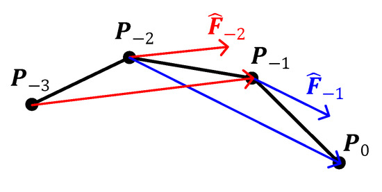
Figure 3.
The principle for solving the approximation of the speed.
The X-axis component of the above equation is
Replacing the in the above equation with the feedrate , the value of can be obtained as
Combining the above equation with Equation (12), the approximation of the tracking error at can be obtained as
Then, the approximation of can be achieved as
Similarly, the approximation of can be obtained as
So far, the approximations of , in the initial conditions of the difference Equation (3) have been achieved.
2.2.3. The Error Analysis and Control of the Approximations of Initial Conditions
In the previous section, an approximation to the initial conditions of the difference Equation (3) was achieved and the error of the approximation led to an error between the output sequence derived from Equation (3) and its true value, which usually will decrease as increases.
Therefore, if the number of sampling points of the final position sequence for nominal acceleration calculation in Figure 1d is set to and the number of sampling points of the position sampling sequence in Equation (1) is set to , when , solving the nominal acceleration according to the last elements of can reduce the error between and its true value.
In order to reduce this error as much as possible, the value of should be as large as possible, but too large a value will take up too much storage space and computation time. Therefore, the error of caused by the approximation error of the initial condition needs to be analyzed to obtain an appropriate value of .
Let the errors between the approximations of , and their true values be and , respectively. Then, it follows from the superposition of the linear and time-invariant system that the error in caused by the approximation error of the initial condition can be regarded as the zero input response of the difference Equation (3) at initial conditions of , namely,
To obtain the expression of , its corresponding characteristic root should be obtained as
According to the value of , the expression of can be divided into the following three cases:
- (1)
- When , are two unequal real numbers and the expression of is
Then, substituting it into Equation (22), the values of can be achieved as
Since in the formula are unknown, substituting into Equation (22) cannot directly calculate the specific value of , but its range can be achieved by inequation scaling. Scaling Equation (22) yields
Similarly, the range of can be obtained from Equations (24) and (A6) as
At this point, let
Then, the following inequation can be obtained from Equation (25):
Therefore, in order to make the position error smaller than the preset upper limit , the following inequation can be obtained:
In this inequation, is the only one unknown symbol. Therefore, the minimum value of that satisfies the inequation can be achieved by traversing the integer (the process can be accelerated by using the bisection method).
- (2)
- When , are two equal real numbers and the expression of is
- (3)
- When , are two unequal complex numbers and the expression of is
For cases (2) and (3), the corresponding can be obtained according to the process of case (1).
So far, the number of sampling points of the Sequence (1) can be obtained as
where has been achieved from Equation (42) below.
At this point, by substituting the in Equation (1) into Equation (3), the output sequence for the X-axis can be obtained. Similarly, the output sequence corresponding to the Y-axis and Z-axis can also be obtained. Then, the output position sequence of the servo system of the three-axis CNC machine tool can be achieved as
In order to reduce the impact on the subsequent calculation, which is caused by the approximation error of the initial conditions, the last terms of the above sequence are taken out and renumbered as
Compared with in Equation (1), achieved here is closer to the actual machining trajectory. At this time, the target values and of the traversed distance in Section 2.1 can be achieved as
where is the preset length of the Sequence (34).
2.3. The Solution of the Nominal Acceleration
According to the position sequence obtained above, the nominal acceleration can be solved. Taking the X-axis as an example, the first-order difference calculation of the in can be performed to obtain the feedrate sequence as
Similarly, the acceleration sequence can be obtained from Equation (36) as
The process of calculating the acceleration sequence is shown in Figure 4a. The midpoint of the sequence is the X-axis component of the acceleration at point . However, since the above differential calculation only uses the position data of a few adjacent interpolation cycles around point , the value of may fluctuate greatly, which will affect the stability of the final nominal acceleration. For this reason, a FIR low-pass filter will be used, as shown in Figure 4b, to process the acceleration sequence of the sampling interval, so as to reduce the fluctuation and obtain a more stable and reasonable nominal acceleration.
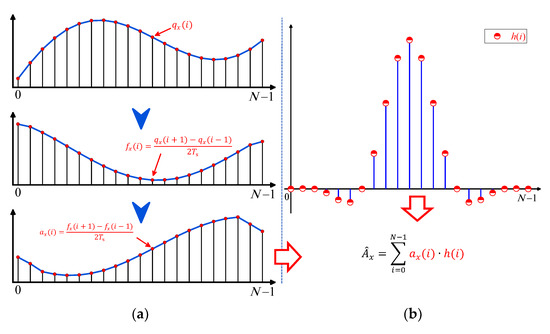
Figure 4.
The process of solving the acceleration of X-axis: (a) the process of calculating the acceleration sequence; (b) the process of filtering the acceleration sequence.
First, the design of the FIR low-pass filter needs to be carried out, which means obtaining the value of in Figure 4b. Let the frequency characteristics of the ideal linear-phase FIR low-pass filter be
where is an imaginary unit, is the cutoff frequency, and is the group delay. By the Fourier inverse transform of , the unit impulse response of the filter can be obtained as
Since in the formula can be taken as any integer, is an infinitely long non-causal sequence, which cannot be used in the actual calculation. In this case, a window function [35,36] needs to be used to truncate . From the data in Table 1, the stopband attenuation in this paper is . Therefore, the Hanning window function with the stopband attenuation −44 dB in Appendix B can meet the requirements, and its expression is
in the above formula can be obtained from the transition bandwidth formula of the Hanning window function, and its value is
where are the sampling frequency, passband cutoff frequency, and stopband start frequency of the FIR low-pass filter, respectively. To ensure that Equation (34) is a position sampling sequence with as the midpoint, must be an odd number; therefore, the obtained from Equation (41) needs to be corrected as

Table 1.
Main parameters used in the simulation and experiment.
So far, the coefficients of the FIR low-pass filter have been obtained as
The unknown in the formula can be obtained from the linear-phase characteristic of the FIR filter as
At this point, in order to check whether the amplitude-frequency characteristics of the designed FIR low-pass filter meet the design requirements, the discrete Fourier transform of can be performed as
Then amplitude-frequency response at is obtained as
If is less than the in Table 1, the designed filter meets the requirement; otherwise, the value of should be increased or another type of window function should be used.
So far, the design of the FIR low-pass filter was completed and the filter coefficients shown in Equation (43) were obtained. By filtering the acceleration Sequence (37), the X-axis acceleration at point can be obtained as
Denoting the filter coefficients, are written in vector form:
The value of can be obtained from Equation (37) and (47) as
Similarly, the acceleration of the Y-axis and Z-axis at the point can be achieved as
Therefore, the nominal acceleration at point can be obtained as
This is the nominal acceleration of the sampling interval with as the midpoint in Figure 1b.
2.4. The Solution of the Feedrate-Constraint Value
In the process of solving the nominal acceleration , shown in Equation (51), the feedrate
remains constant and the tangential acceleration is 0. Therefore, the nominal acceleration is the normal acceleration, so that the nominal radius of curvature of the continuous small line segments in the sampling interval can be calculated as
At this point, assume that the small line segments of the sampling interval are machined at another feedrate and the normal acceleration generated under the action of the nominal radius of curvature is just equal to the maximum allowable value of the normal acceleration , namely,
Then, is the feedrate-constraint value at point and its value is
So far, the feedrate-constraint value at any corner of the continuous small line segments can be obtained from the proposed FNA method. Then, combined with the conventional feedrate planning [18,37,38] and interpolation methods, the CNC machining of the continuous small line segments can be realized.
3. Simulation and Experimental Results
In order to verify the effectiveness of the FNA method proposed in this paper, the algorithm simulation and machining experiment will be conducted in this section. The algorithm simulation was performed on a personal computer with the CPU i3-9100F, while the machining experiment was performed on a three-axis CNC machine tool DC-6060A (KAIBO, Ningbo, China) controlled by a self-developed controller. The X/Y/Z axes travel of the machine tool were 600/600/260 mm, respectively. The architecture of the experimental platform is shown in Figure 5.
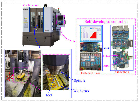
Figure 5.
The architecture of the experimental platform.
The Embedded Linux controller iTop4412 (TOPEET, Beijing, China) in the figure was mainly used for GUI, while the ARM (STM32H743) controller ran CNC algorithms, including ISO6983 code parsing, nominal acceleration solving, feedrate planning, interpolation, etc. The FPGA (EP4CE22) was mainly used for fine interpolation and generating control signals for servo drives.
The main parameters used in the simulation and experiment and their default values are shown in Table 1.
In the actual CNC machining, the angle-constraint method is easy to realize and simple to calculate and it is the most widely used method to calculate the feedrate-constraint value. Therefore, the simulation and experiment were mainly performed on the angle-constraint method and the proposed FNA method.
3.1. 2D Machining Simulation
The 2D machining path shown in Figure 6 contains corners, arcs, and reversals, which are typical and complex. Therefore, it can be used for the simulation to compare the effect of the angle-constraint method and FNA method.
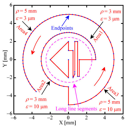
Figure 6.
The 2D machining path of the continuous small line segments.
The radius of curvature at Area1 the in above figure is , and the curve here is discretized into small continuous line segments with the chord error . Therefore, the angle of the corner of adjacent segments is
Therefore, the feedrate-constraint value obtained by using the virtual transition-arc constraint method [11] is
while, according to the constraint of the radius of curvature and the normal acceleration, the feedrate-constraint value should be
Similarly, the feedrate-constraint values at Area2, Area3, and Area4 can also be achieved, as shown in Table 2.
Table 2.
Geometric information of the machining path and its feedrate-constraint value.
The angle-constraint method and the FNA method were used to calculate the feedrate-constraint value of the machining path in Figure 6, respectively. Then, the feedrate planning and interpolation were performed, and the results are shown in Figure 7.
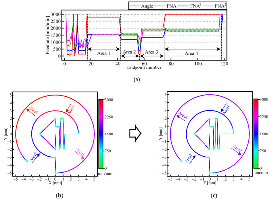
Figure 7.
The feedrate planning results of the 2D machining path: (a) the feedrate-constraint value obtained from different methods (FNA 1: The FNA method without the trajectory prediction. FNA 2: The FNA method without the acceleration filtering); (b) the feedrate planning result of the angle-constraint method; (c) the feedrate planning result of the FNA method.
As can be seen from Figure 7a, for Line Area in Figure 6, both the angle-constraint method and the FNA method effectively constrained the feedrate, while for Curve Area, the feedrate-constraint values obtained from these two methods were significantly different. The machining paths in Area1 and Area2 (or Area3 and Area4) had the same radius of curvature, but the angles were different. Therefore, if the angle-constraint method is used to calculate the feedrate-constraint value, the machining paths with the same radius of curvature will be machined by different feedrates, as shown in Figure 7b. Especially in Area1 and Area4, the feedrate exceeded the theoretical value obtained by Equation (58). While in Area1–Area4 of Figure 7c, the feedrates obtained based on the FNA method were all nearly same as the theoretical values in Table 2.
In addition, the small line segments in Area2 and Area3 were relatively longer; so, the velocity direction changed more at the corner. As a result, in Figure 7a, the feedrate-constraint value obtained by the FNA 1 method was obviously lower than the theoretical value, while the feedrate-constraint value obtained by the FNA method was almost equal to the theoretical value, which verified the effectiveness of the machining trajectory prediction in Section 2.2. Therefore, the machining trajectory prediction can suppress the accuracy problem of continuous small line segments and make the calculating results of the proposed method more reasonable and stable. Similarly, the feedrate-constraint values obtained by the FNA 2 method in Area1 and Area2 (or Area3 and Area4) had a difference over 50 mm/min, while the difference of the FNA method was less than 10 mm/min, which verified the effectiveness of the acceleration filtering in Section 2.3.
In summary, the proposed FNA method was not sensitive to the length of the line segment, the angle of the corner, etc. The proposed method was stable and the obtained feedrate-constraint value was more reasonable.
3.2. 3D Machining Simulation
The effectiveness of the FNA method was preliminarily verified by the 2D simulation in the previous section. In this section, the FNA method will be further simulated and analyzed by using the continuous small line segments of a 3D free-form surface.
For the first 3000 lines of the ISO6983 code [39] corresponding to the machining path shown in Figure 8b, the angle-constraint method, the curvature-constraint method, the acceleration-constraint method [17], and the proposed FNA method were used to calculate the feedrate-constraint value, respectively. Then, the feedrate planning and interpolation were performed, and the final feedrate results are shown in Figure 9.
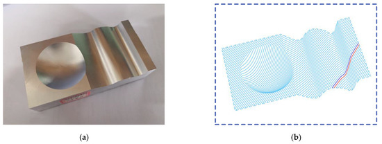
Figure 8.
The workpiece and its machining path: (a) the workpiece; (b) the machining path (simplified).
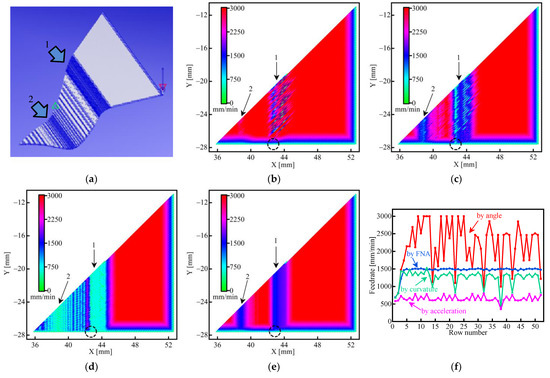
Figure 9.
The feedrate results of the 3D machining path: (a) the line segments of the free-form surface; the feedrate results of the (b) angle-constraint, (c) curvature-constraint, (d) acceleration-constraint and (e) FNA method; (f) the feedrate of each row when X = 43 mm.
For area 1 with large curvature in Figure 9a, the distribution of the feedrate in the X-Y plane obtained by the angle-constraint method is shown in Figure 9b, and the feedrate was distributed from 500 mm/min to 3000 mm/min, which is rather chaotic. In a contrast, the feedrate obtained from the FNA method is shown in Figure 9e, which was maintained around 1500 mm/min, and the stability of the feedrate was obviously better than the one of the angle-constraint method and the other two constraint methods.
In order to quantify the stability of the feedrate to make a better comparison between different methods, the feedrate values for each row at X = 43 mm are collected in Figure 9b–e, respectively, and their distribution is shown in Figure 9f. The average, range, relative range (range/average), and standard deviation were calculated (the first three points in the circles of Figure 9b–f are in the reverse region and were not taken into the statistics), and the results are shown in Table 3.
Table 3.
The statistics results of the feedrate of each row when X = 43 mm.
From the data in this table, it can be seen that the proposed FNA method worked much better than other three methods. Especially compared with the angle-constraint method, the FNA method reduced the relative range of the feedrate from 90.8% to 4.3%, and the standard deviation also decreased from 602 to 17. Therefore, the feedrate obtained by the FNA method had better stability, which is quite important for improving the CNC machining quality of the free-form surface.
3.3. Experiment
The numerical analysis in the simulations verified the effectiveness of the FNA method, while this section will use the experiment to verify the effectiveness of the FNA method more directly. For the machining path shown in Figure 8b, the feedrate was constrained by the angle-constraint method and FNA method, respectively, and the CNC machining was performed under the same machining conditions. In the machining, a ball milling cutter W2QX4408 (Weidiao, Shanghai, China) was used, and the machining material was AlMg1SiCu aluminum. The command feedrates were both 3000 mm/min, and the machining results are shown in Figure 10.
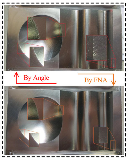
Figure 10.
The machining results of the angle-constraint method and FNA method.
When the angle-constraint method was used, the obtained feedrate was overlarge and unstable and the overcutting occurred at many places, resulting in machining damage represented by “pits”. However, when the FNA method was used, the obtained feedrate was reasonable and stable and the machining quality was obviously improved. In addition, the machining times of the two methods were 22 min 45 s and 22 min 8 s, respectively. Therefore, the proposed FNA method can both improve the machining efficiency and the machining quality. The machining experiments and algorithm simulations corroborate each other and they both verify the effectiveness of the FNA method proposed in this paper.
4. Conclusions
The conventional feedrate-constraint method is sensitive to the angle of the corner and the length of the line segment, and the feedrate-constraint value obtained is unreasonable, which will result in damages to the machining quality. In this paper, the FNA method was proposed, in which the line segment path sampling, the machining trajectory prediction, and the acceleration filtering were used, and they can significantly improve the reasonableness and stability of the feedrate-constraint value.
In the simulation of the 2D machining path, the feedrate-constraint value obtained by the FNA method was more stable and reasonable compared with the angle-constraint method, and was almost equal to the theoretical value. In the simulation of the 3D machining path of the free-form surface, compared with the angle-constraint method, the relative range of the feedrate obtained by the FNA method decreased from 90.8% to 4.3% and the standard deviation decreased from 602 to 17, which means that the stability of the feedrate was significantly improved. Compared with the curvature-constraint method and acceleration-constraint method, the proposed method also worked much better. The machining experiments showed that the proposed FNA method ran stably and can both reduce the machining time and improve the machining quality, thus helping to promote the application of the continuous small line segments in the high-speed and high-precision CNC machining.
In view of the limited time, the FNA method only worked for line segments. It will be improved to be applicable for the machining path consisting of the line segment, the arc, and the parametric curve. Additionally, the current method was only implemented in the three-axis CNC machining and has not yet been applied to the five-axis, which will be realized in the future.
Author Contributions
Conceptualization, P.G., Y.W., and R.W.; methodology, P.G. and R.W.; soft-ware, P.G.; validation, P.G., Z.S., H.Z., and P.Z.; writing—original draft preparation, P.G. and R.W.; writing—review and editing, P.G., Y.W., and F.L.; visualization, H.L.; project administration, Y.W.; funding acquisition, Y.W. All authors have read and agreed to the published version of the manuscript.
Funding
This research was sponsored by National Natural Science Foundation of China (No.51275462) and Science and Technology Innovation 2025 Major Project of Ningbo (No.2018B10069).
Institutional Review Board Statement
Not applicable.
Informed Consent Statement
Not applicable.
Data Availability Statement
The data presented in this study are available on request from the corresponding author.
Conflicts of Interest
The authors declare no conflict of interest.
Nomenclature
| FNA | The proposed Feedrate-constraint method based on Nominal Acceleration |
| Line Area | Area with long line segments in the machining path |
| Curve Area | Area with continuous small line segments discretized from the curve in the machining path |
| The feedrate-constraint value at the corner of adjacent line segments | |
| The const feedrate used for machining the small line segments in FNA method | |
| Position sampling sequence of the sampling interval | |
| The length of the sequence | |
| Predicted position sequence corresponding to | |
| The length of the sequence | |
| Nominal acceleration corresponding to a corner | |
| Interpolation period and sampling period | |
| Normal acceleration |
Appendix A
According to the working principle of the servo system, the following two properties were easily obtained:
Property 1: When the X-axis remains stationary, the input position sequence is a constant value and the output position sequence must also be the same constant value.
Property 2: When the X-axis moves at a constant speed, the tracking error must be a constant value [33] and is positively correlated with the speed. Then, the following equation can be achieved from Property 1 and Equation (3):
It can be seen from Property 2 that when the X-axis moves at a constant speed, the following equation can be obtained:
Substituting the equation into Equation (3), the value of can be achieved as
Assuming that the speed of the X-axis is , the following equation can be obtained:
Substituting this into Equation (A3), the value of can be obtained as
It can be seen from Equation (A1) that the value of the numerator of the first item in Equation (A5) is 0, so the value of is
in which
It follows that when the X-axis moves at a constant speed, the tracking error is proportional to the speed and the scale factor is .
Appendix B
Table A1.
Several commonly used window functions in the design of the FIR filter [35,36].
Table A1.
Several commonly used window functions in the design of the FIR filter [35,36].
| Window Name | Expression | Transition Width | Minimum Stopband Attenuation |
|---|---|---|---|
| Rectangular | 1.8 | −21 | |
| Hanning | 6.2 | −44 | |
| Hamming | 6.6 | −53 | |
| Blackman | 11 | −74 |
References
- Tajima, S.; Sencer, B. Global tool-path smoothing for CNC machine tools with uninterrupted acceleration. Int. J. Mach. Tools Manuf. 2017, 121, 81–95. [Google Scholar] [CrossRef]
- Liu, Y.; Wan, M.; Qin, X.B.; Xiao, Q.B.; Zhang, W.H. FIR filter-based continuous interpolation of G01 commands with bounded axial and tangential kinematics in industrial five-axis machine tools. Int. J. Mech. Sci. 2020, 169, 105325. [Google Scholar] [CrossRef]
- Xiao, Q.B.; Wan, M.; Qin, X.B.; Liu, Y.; Zhang, W.H. Real-time smoothing of G01 commands for five-axis machining by constructing an entire spline with the bounded smoothing error. Mech. Mach. Theory 2021, 161, 104307. [Google Scholar] [CrossRef]
- Zhang, Y.; Zhao, M.Y.; Ye, P.Q.; Zhang, H. A G4 continuous B-spline transition algorithm for CNC machining with jerk-smooth feedrate scheduling along linear segments. Comput.-Aided Des. 2019, 115, 231–243. [Google Scholar] [CrossRef]
- Xiao, Q.B.; Wan, M.; Liu, Y.; Qin, X.B.; Zhang, W.H. Space corner smoothing of CNC machine tools through developing 3D general clothoid. Robot. Comput.-Integr. Manuf. 2020, 64, 101949. [Google Scholar] [CrossRef]
- Fan, W.; Ji, J.W.; Wu, P.Y.; Wu, D.Z.; Chen, H. Modeling and simulation of trajectory smoothing and feedrate scheduling for vibration-damping CNC machining. Simul. Model. Pract. Theory 2020, 99, 102028. [Google Scholar] [CrossRef]
- Tsai, M.S.; Huang, Y. A novel integrated dynamic acceleration/deceleration interpolation algorithm for a CNC controller. Int. J. Adv. Manuf. Technol. 2016, 87, 279–292. [Google Scholar] [CrossRef]
- Shahzadeh, A.; Khosravi, A.; Robinette, T.; Nahavandi, S. Smooth path planning using biclothoid fillets for high speed CNC machines. Int. J. Mach. Tools Manuf. 2018, 132, 36–49. [Google Scholar] [CrossRef]
- Hu, J.; Xiao, L.J.; Wang, Y.H.; Wu, Z.Y. An optimal feedrate model and solution algorithm for a high-speed machine of small line blocks with look-ahead. Int. J. Adv. Manuf. Technol. 2006, 28, 930–935. [Google Scholar] [CrossRef]
- Luo, F.Y.; Zhou, Y.F.; Yin, J. A universal velocity profile generation approach for high-speed machining of small line segments with look-ahead. Int. J. Adv. Manuf. Technol. 2007, 35, 505–518. [Google Scholar] [CrossRef]
- Zhang, D.L.; Zhou, L.S. Adaptive Algorithm for Feedrate Smoothing of High Speed machining. Acta Aeron-Autica Astronaut. Sin. 2006, 27, 125–130. [Google Scholar]
- Zhang, Y.; Ye, P.Q.; Tang, J.J.; Zhang, H. Real-time look-ahead feedrate planning algorithm of short line segment based on planning unit. Comput. Integr. Manuf. Syst. 2017, 23, 2483–2490. [Google Scholar]
- Syntec. SYNTEC CNC Parameters; Syntec Technology, Inc.: Brea, CA, USA, 2018. [Google Scholar]
- Dong, J.C.; Wang, T.Y.; Li, B.; Ding, Y.Y. Smooth feedrate planning for continuous short line tool path with contour error constraint. Int. J. Mach. Tools Manuf. 2014, 76, 1–12. [Google Scholar] [CrossRef]
- Su, Z.W.; Zhou, H.C.; Hu, P.C.; Fan, W. Three-axis CNC machining feedrate scheduling based on the feedrate restricted interval identification with sliding arc tube. Int. J. Adv. Manuf. Technol. 2018, 99, 1047–1058. [Google Scholar] [CrossRef]
- FANUC. Parameter Manual; Fanuc Automation North America, Inc.: Charlottesville, VA, USA, 2004. [Google Scholar]
- Wang, L.; Cao, J.F. A look-ahead and adaptive speed control algorithm for high-speed CNC equipment. Int. J. Adv. Manuf. Technol. 2012, 63, 705–717. [Google Scholar] [CrossRef]
- Obukhov, A.I.; Martinova, L.I.; Lyubimov, A.B. Developing of the Look Ahead Algorithm for Linear and Nonlinear Laws of Control of Feedrate in CNC. Autom. Remote Control 2020, 81, 380–386. [Google Scholar] [CrossRef]
- Li, J.G.; Wu, X.L.; Li, Z.X.; Zhou, L. A blended feedrate planning algorithm for continuous toolpath. J. Harbin Inst. Technol. 2009, 41, 29–32. [Google Scholar]
- Jahanpour, J. High speed contouring enhanced with C2 PH quintic spline curves. Sci. Iran. 2012, 19, 311–319. [Google Scholar] [CrossRef] [Green Version]
- Zhao, H.; Zhu, L.M.; Ding, H. A real-time look-ahead interpolation methodology with curvature-continuous B-spline transition scheme for CNC machining of short line segments. Int. J. Mach. Tools Manuf. 2013, 65, 88–98. [Google Scholar] [CrossRef]
- Beudaert, X.; Lavernhe, S.; Tournier, C. 5-axis local corner rounding of linear tool path discontinuities. Int. J. Mach. Tools Manuf. 2013, 73, 9–16. [Google Scholar] [CrossRef] [Green Version]
- Sun, S.J.; Lin, H.; Zheng, L.M.; Yu, J.G.; Hu, Y. A real-time and look-ahead interpolation methodology with dynamic B-spline transition scheme for CNC machining of short line segments. Int. J. Adv. Manuf. Technol. 2016, 84, 1359–1370. [Google Scholar] [CrossRef]
- Wang, Y.S.; Yang, D.S.; Liu, Y.Z. A real-time look-ahead interpolation algorithm based on Akima curve fitting. Int. J. Mach. Tools Manuf. 2014, 85, 122–130. [Google Scholar] [CrossRef]
- Du, X.; Huang, J.; Zhu, L.M.; Ding, H. An error-bounded B-spline curve approximation scheme using dominant points for CNC interpolation of micro-line toolpath. Robot. Comput.-Integr. Manuf. 2020, 64, 101930. [Google Scholar] [CrossRef]
- Piegl, L.A.; Tiller, W. The NURBS Book, 2nd ed.; Springer: Berlin/Heidelberg, Germany, 1997. [Google Scholar]
- Ueng, W.D.; Lai, J.Y.; Tsai, Y.C. Unconstrained and constrained curve fitting for reverse engineering. Int. J. Adv. Manuf. Technol. 2007, 33, 1189–1203. [Google Scholar] [CrossRef]
- Siemens. Milling with SINUMERIK 5-Axis Machining Manual; Siemens: Erlangen, Germany, 2009. [Google Scholar]
- Tajima, S.; Sencer, B. Kinematic corner smoothing for high speed machine tools. Int. J. Mach. Tools Manuf. 2016, 108, 27–43. [Google Scholar] [CrossRef]
- Lin, K.Y.; Ueng, W.D.; Lai, J.Y. CNC codes conversion from linear and circular paths to NURBS curves. Int. J. Adv. Manuf. Technol. 2008, 39, 760–773. [Google Scholar] [CrossRef]
- Zhang, Y.; Ye, P.Q.; Zhao, M.Y.; Zhang, H. Dynamic feedrate optimization for parametric toolpath with data-based tracking error prediction. Mech. Syst. Signal Proc. 2019, 120, 221–233. [Google Scholar] [CrossRef]
- Chiu, T.C.; Tomizuka, M. Contouring Control of Machine Tool Feed Drive Systems: A Task Coordinate Frame Approach. IEEE Trans. Control. Syst. Technol. 2001, 9, 130–139. [Google Scholar] [CrossRef]
- Jin, F.M.; Deng, Z.P. The Dynamic Performance and Steady-state Performance for the Close-loop Servo System. Modul. Mach. Tools Autom. Manuf. Tech. 2006, 6, 38–39. [Google Scholar]
- Renton, D.; Elbestawi, M.A. High speed servo control of multi-axis machine tools. Int. J. Mach. Tools Manuf. 2000, 40, 539–559. [Google Scholar] [CrossRef] [Green Version]
- Gazi, O. Understanding Digital Signal Proccessing; Springer: Berlin/Heidelberg, Germany, 2018. [Google Scholar]
- Schlichthärle, D. Digital Filters: Basics and Design; Springer: Berlin/Heidelberg, Germany, 2011. [Google Scholar]
- Huang, J.; Du, X.; Zhu, L.M. Feasibility of the Bi-Directional Scanning Method in Acceleration/deceleration Feedrate Scheduling for CNC Machining. In Proceedings of the 10th International Conference Intelligent Robotics and Applications (ICIRA), Wuhan, China, 16–18 August 2017; pp. 171–183. [Google Scholar]
- Ni, H.P.; Hu, T.L.; Zhang, C.R.; Ji, S.; Chen, Q.Z. An optimized feedrate scheduling method for CNC machining with round-off error compensation. Int. J. Adv. Manuf. Technol. 2018, 97, 2369–2381. [Google Scholar] [CrossRef]
- Guo, P. The NC File of A Composited Free-Form Surface. Available online: https://github.com/guodepeng/cnc_git/blob/master/WAVE_R2_copy.NC (accessed on 2 July 2021).
Publisher’s Note: MDPI stays neutral with regard to jurisdictional claims in published maps and institutional affiliations. |
© 2021 by the authors. Licensee MDPI, Basel, Switzerland. This article is an open access article distributed under the terms and conditions of the Creative Commons Attribution (CC BY) license (https://creativecommons.org/licenses/by/4.0/).