
Card3DFace—An Application to Enhance 3D Visual Validation in ID Cards and Travel Documents


Abstract
:1. Introduction
2. Related Work
2.1. Three-Dimensional Face Reconstruction
2.2. Head Model Reconstruction and Filtering
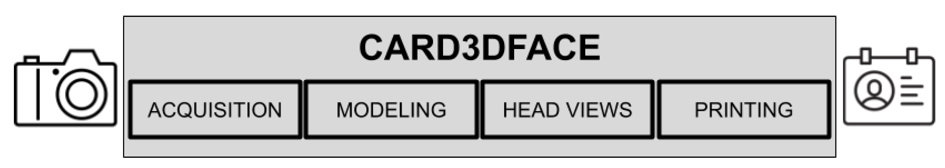
3. System Building Blocks
3.1. Acquisition
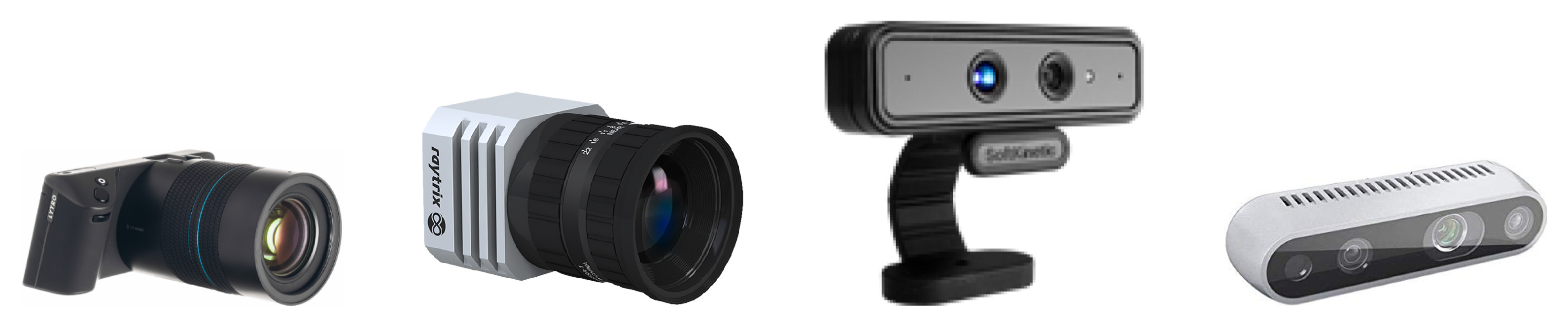
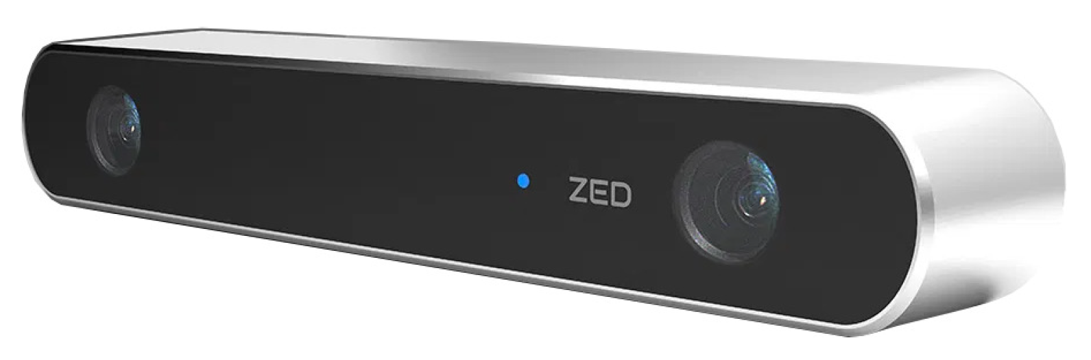
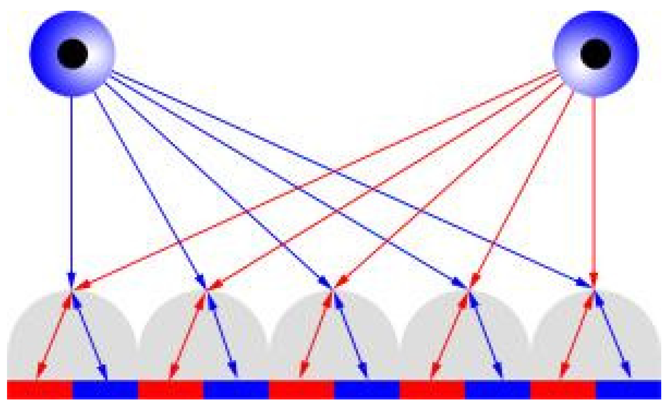
3.1.1. Studied Camera Types Technologies and Selection
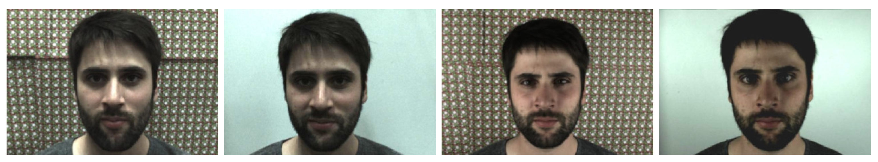
3.1.2. Set-Up for Image Acquisition Conditions
3.2. Modeling
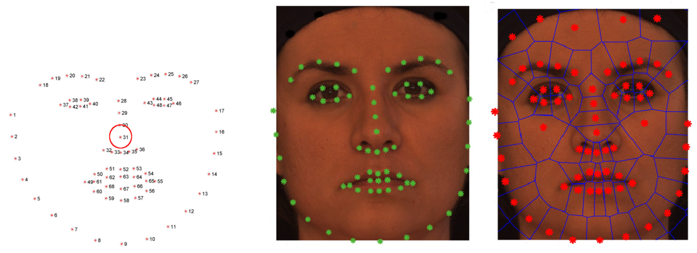
3.2.1. Reconstruction
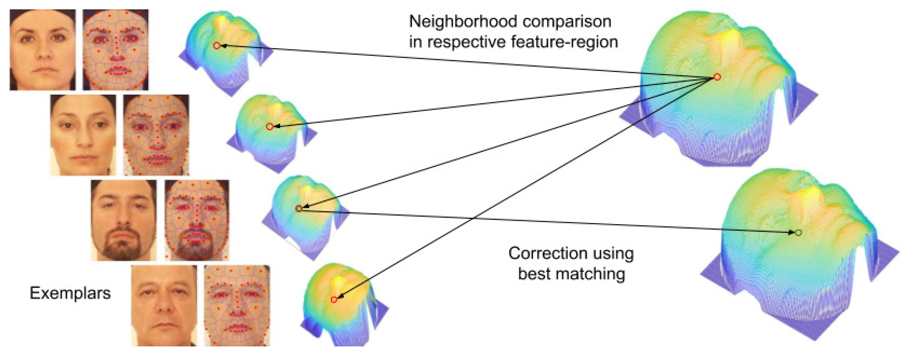
3.2.2. Filtering
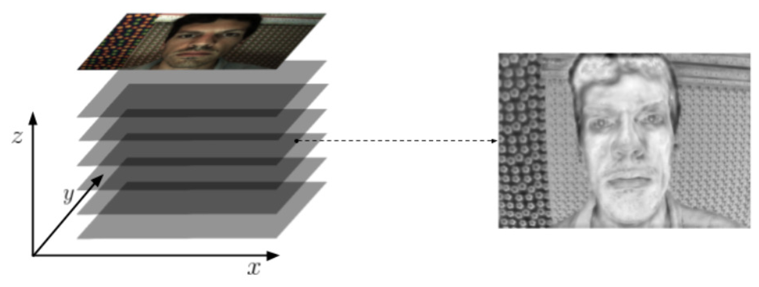
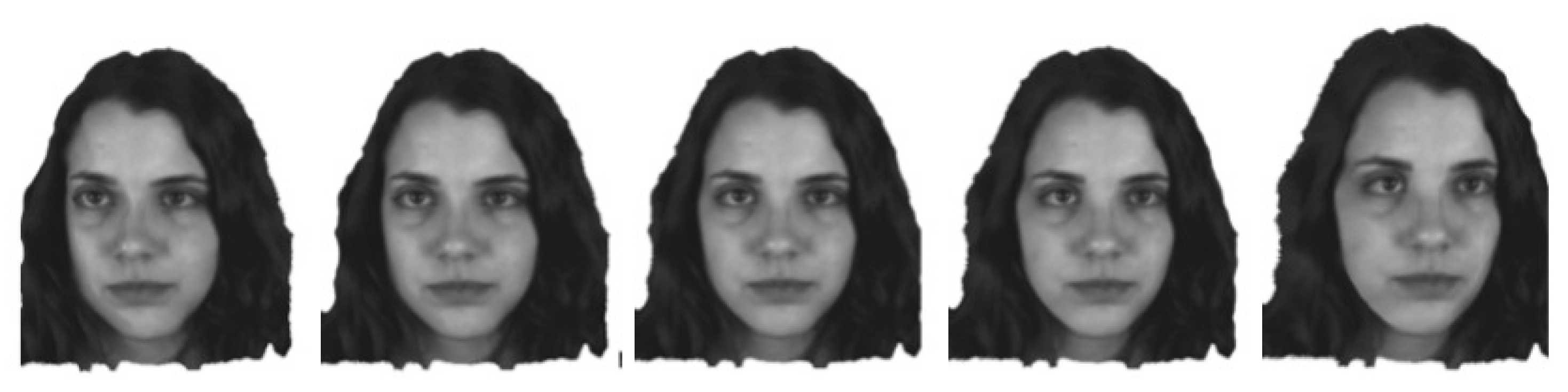
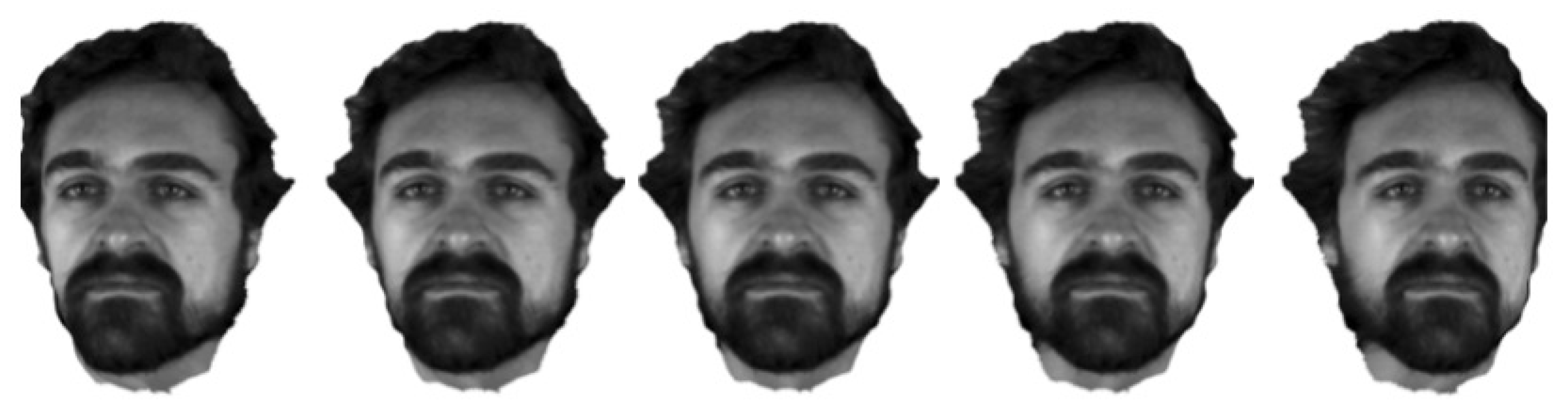
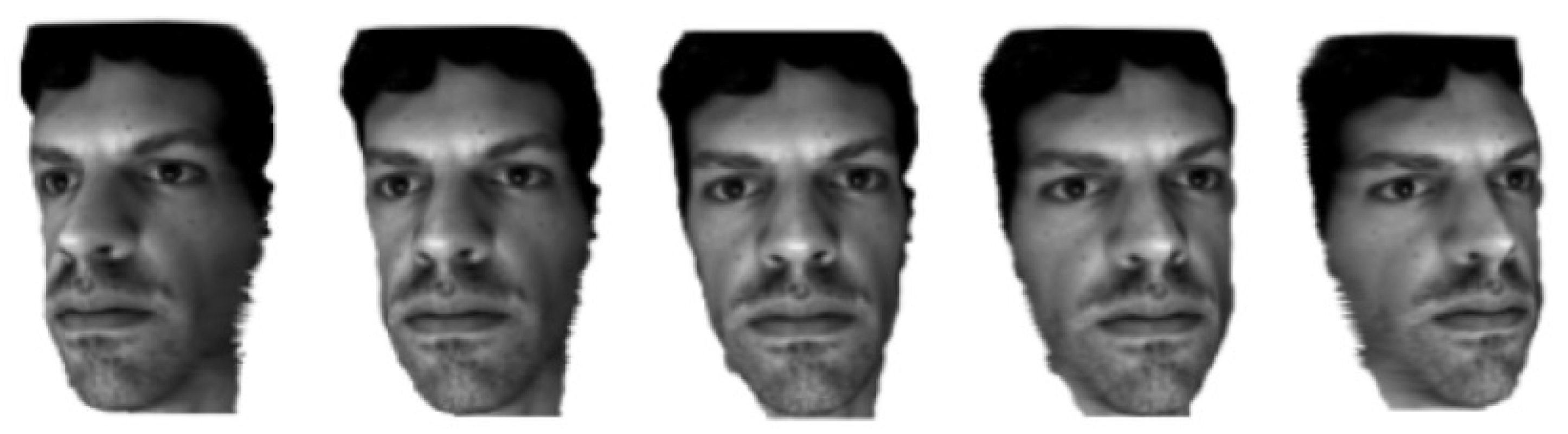
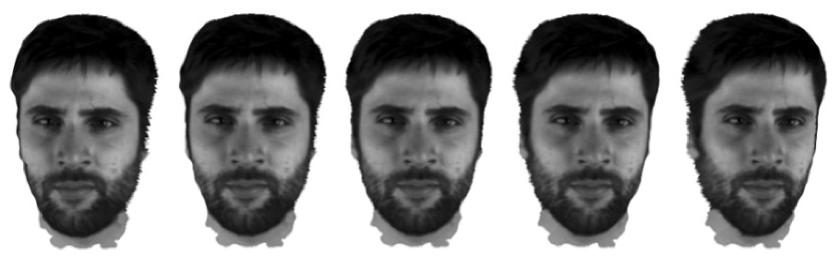
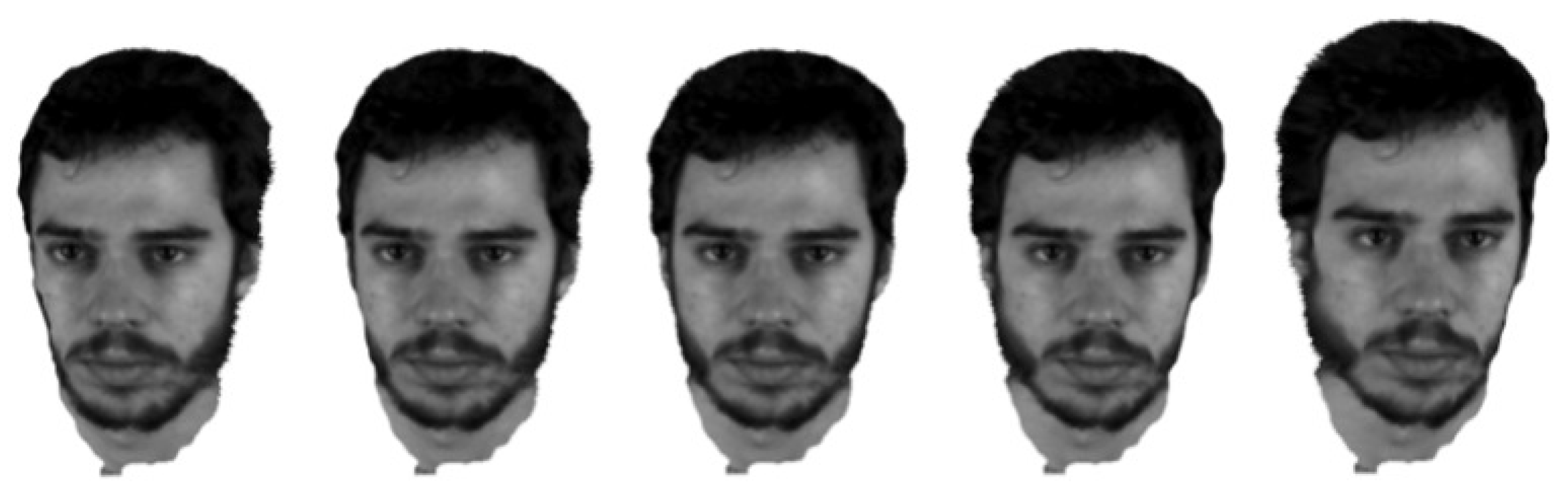
3.3. Head Views
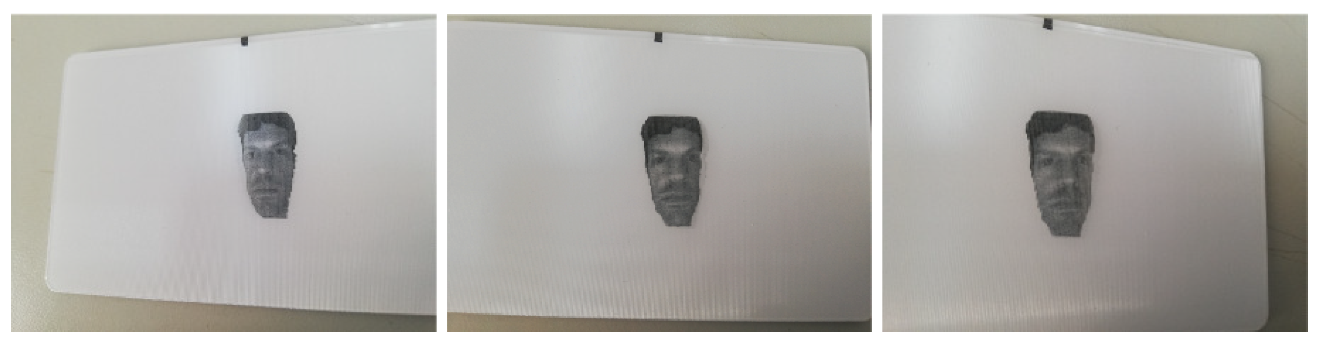
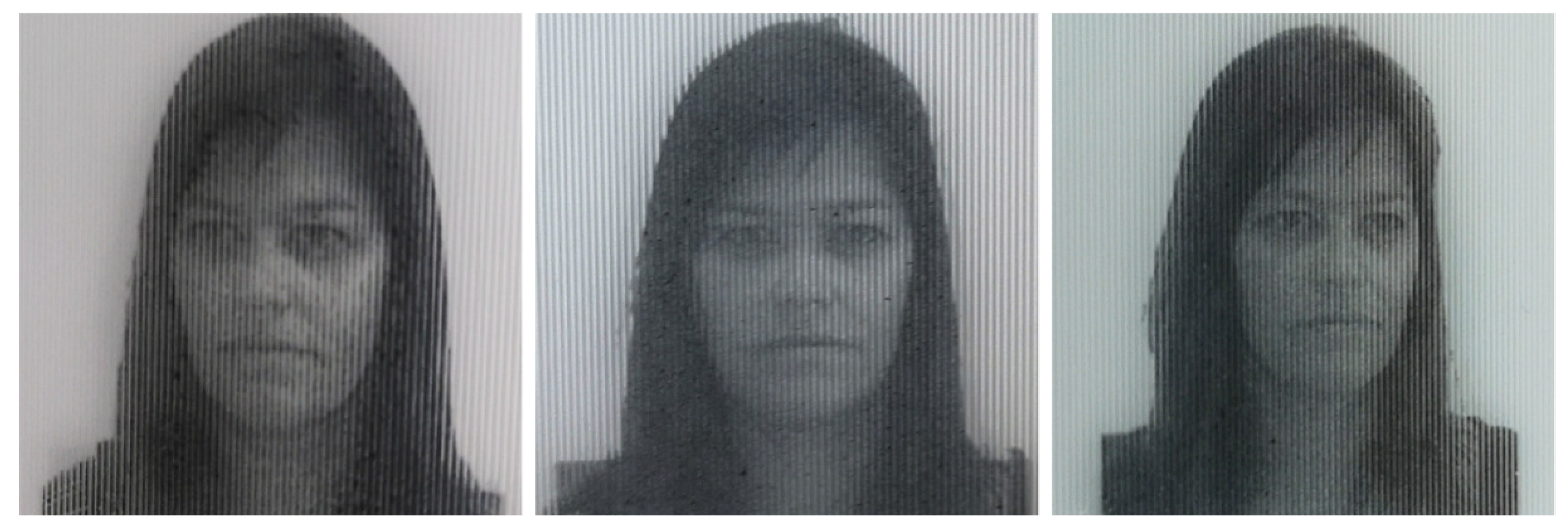
3.4. Lenticular Printing
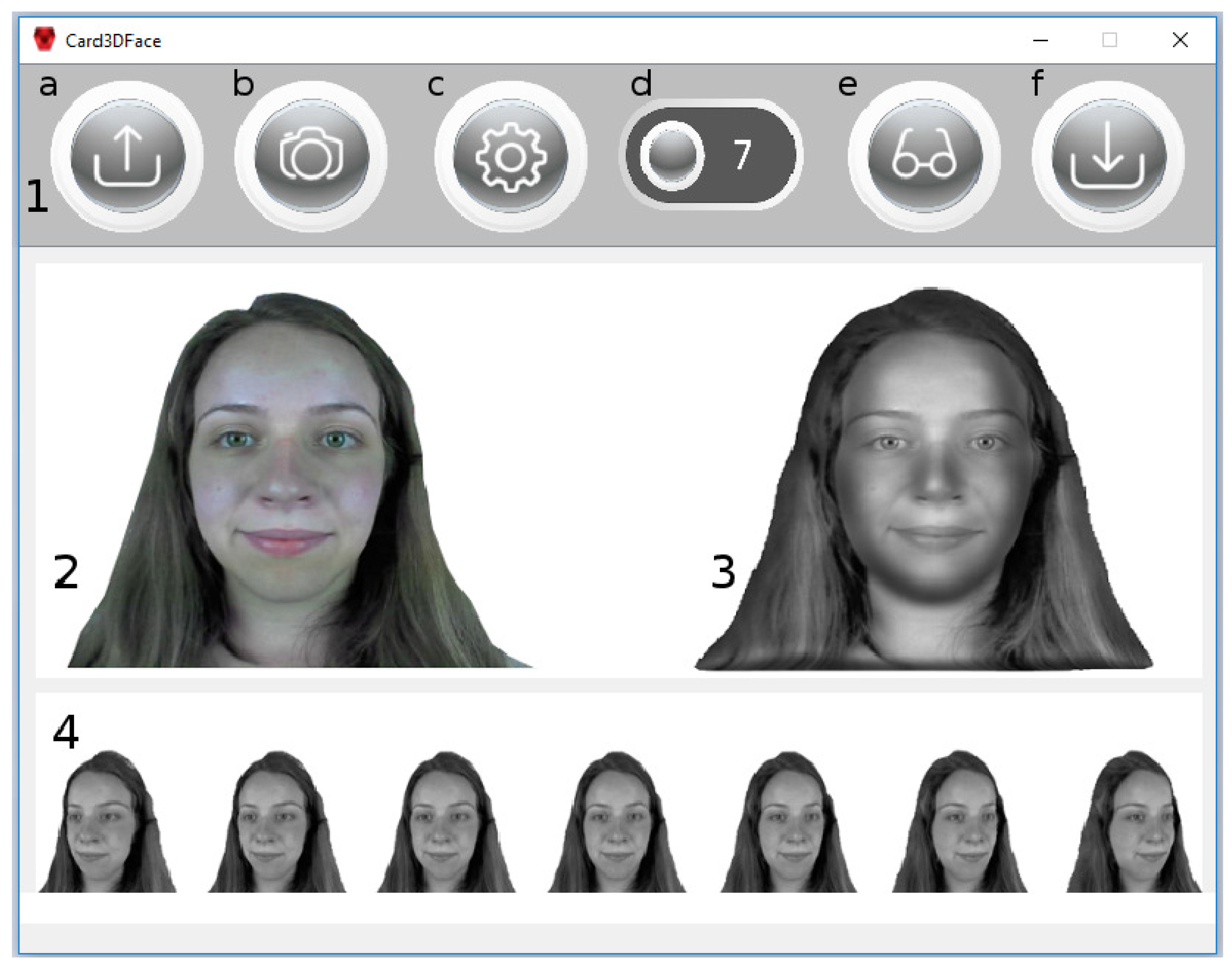
4. Application Interface
5. Experiments and Results
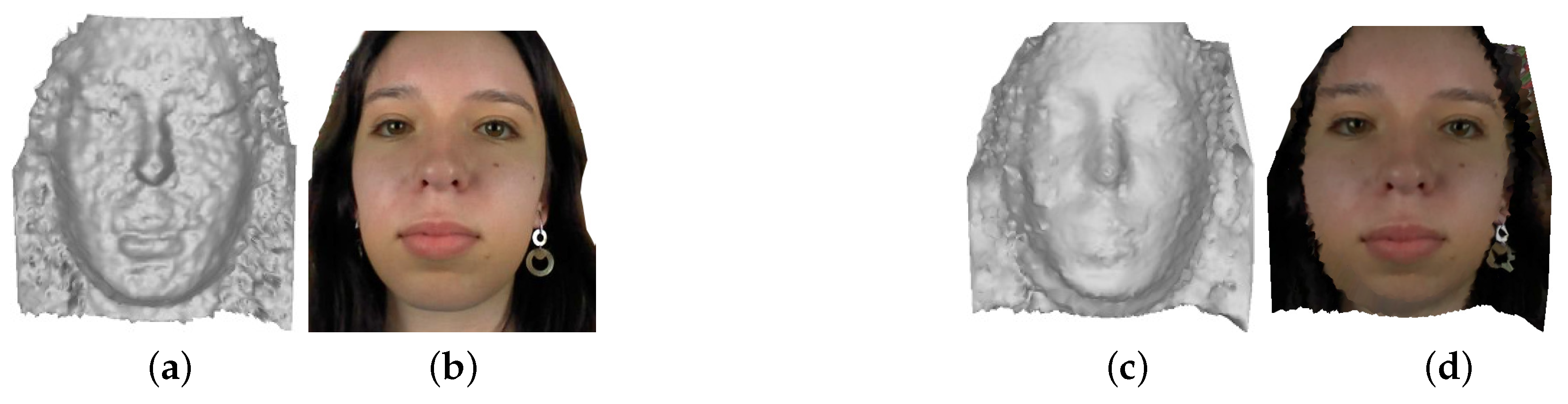
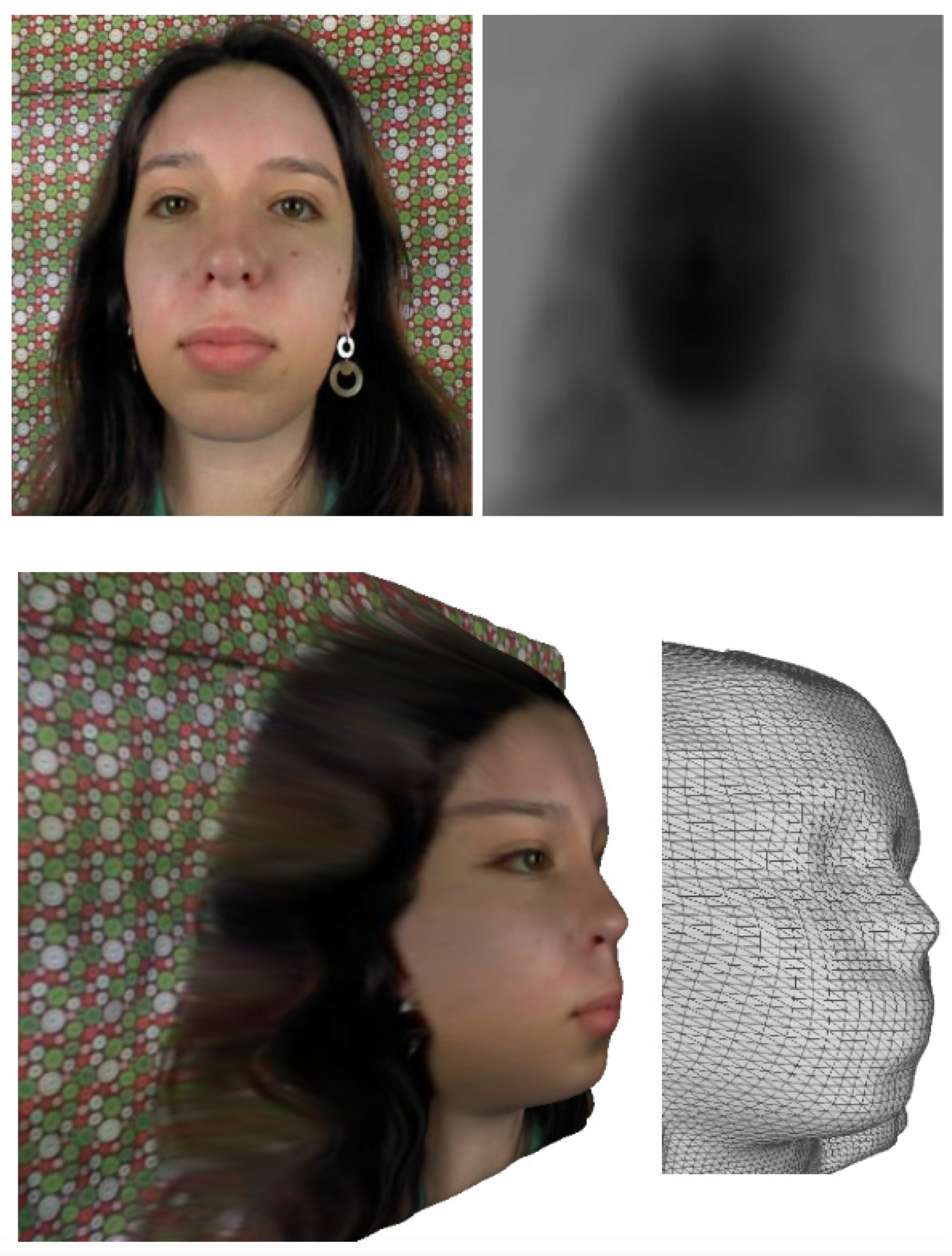
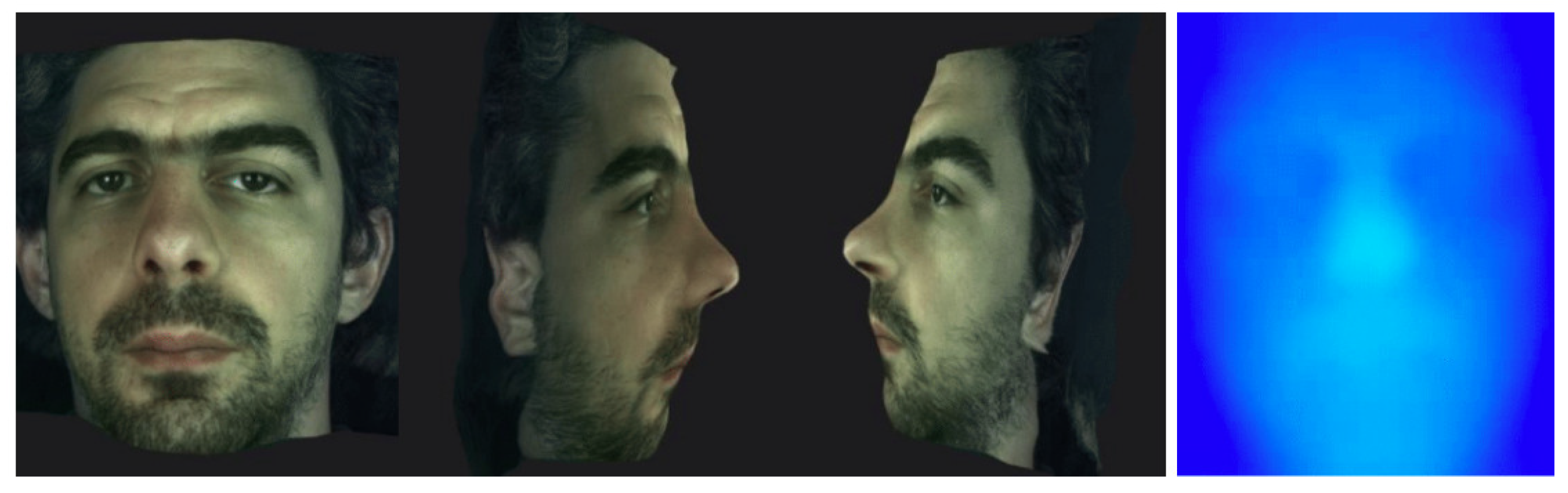
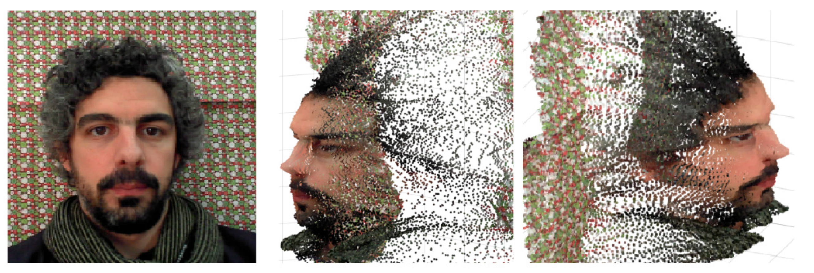
5.1. Reconstruction Evaluation
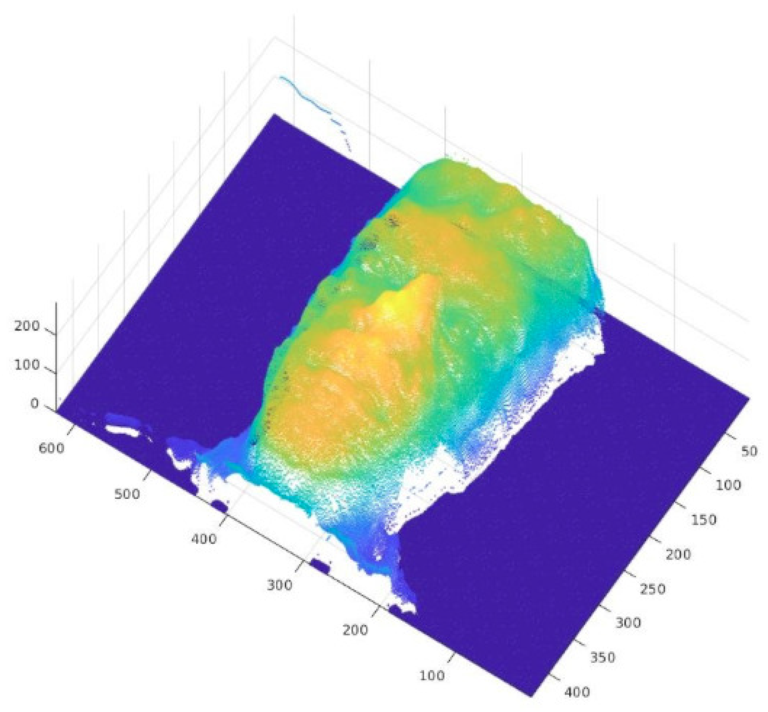
5.1.1. Three-Dimensioanl Reconstruction Model—Lytro Illum
5.1.2. Three-Dimensional Reconstruction Model—Raytrix
5.1.3. Three-Dimensional Reconstruction Model—Time of Flight
5.1.4. Three-DImensional Reconstruction Model—Stereo
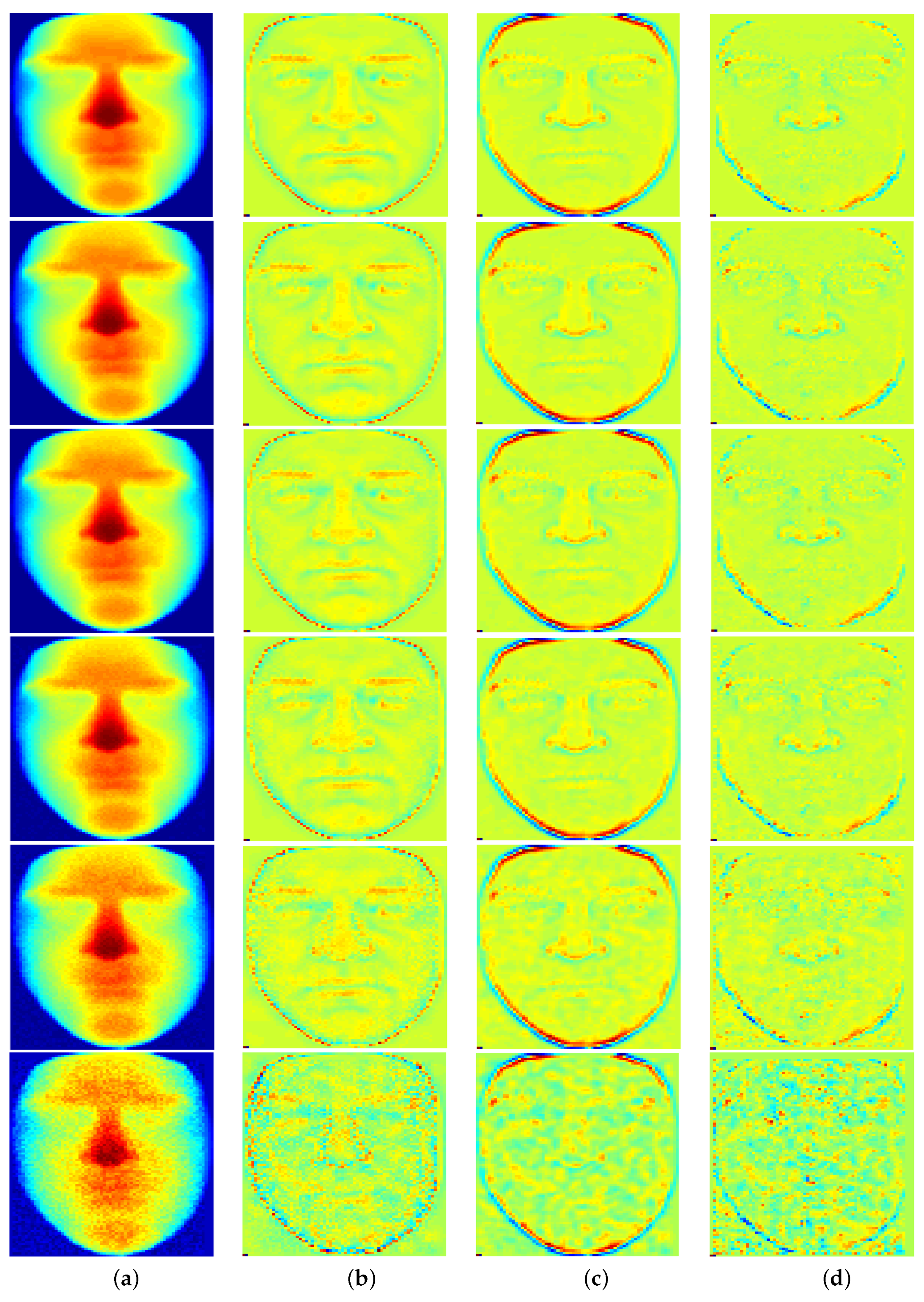
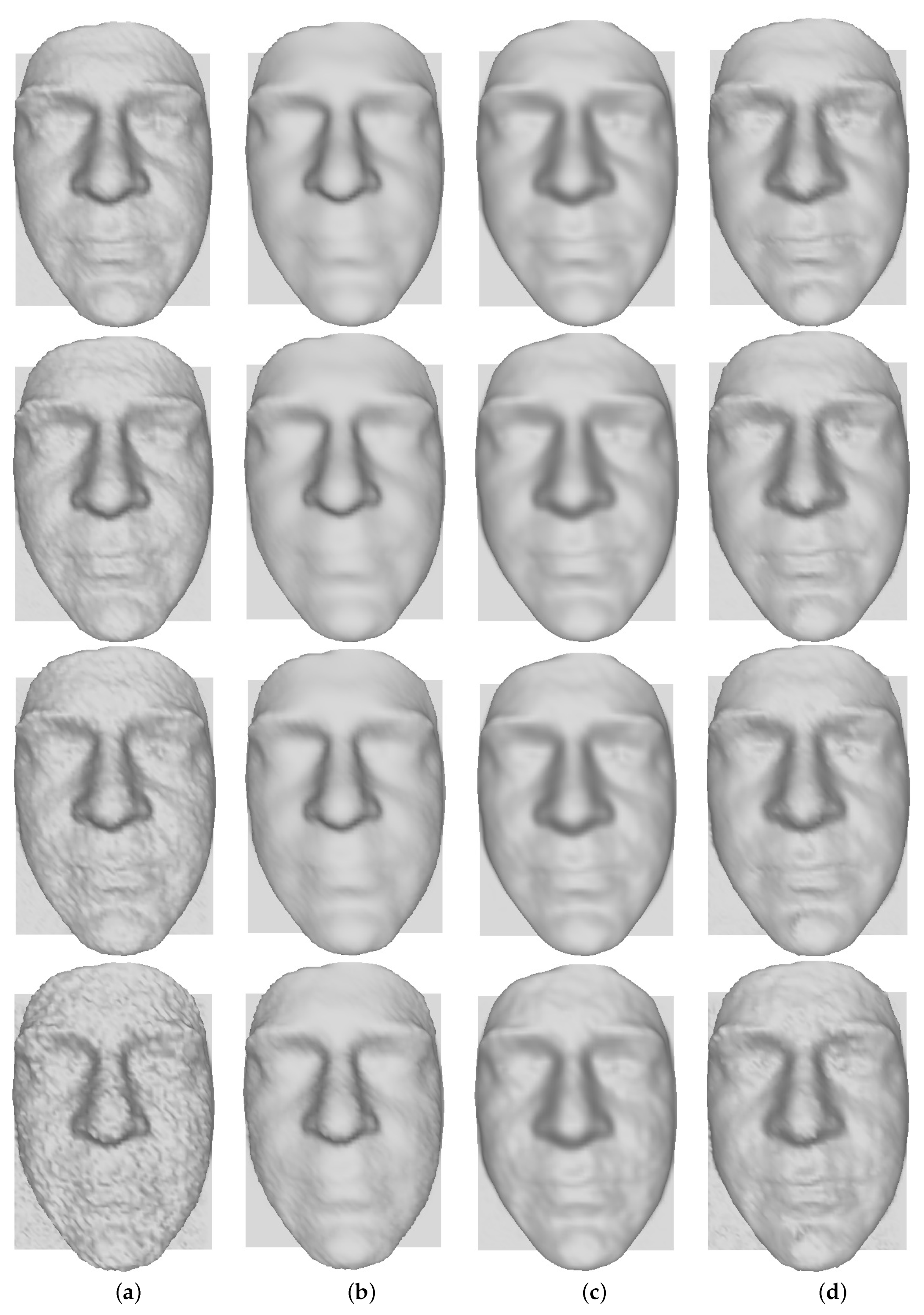
5.2. Filtering Evaluation
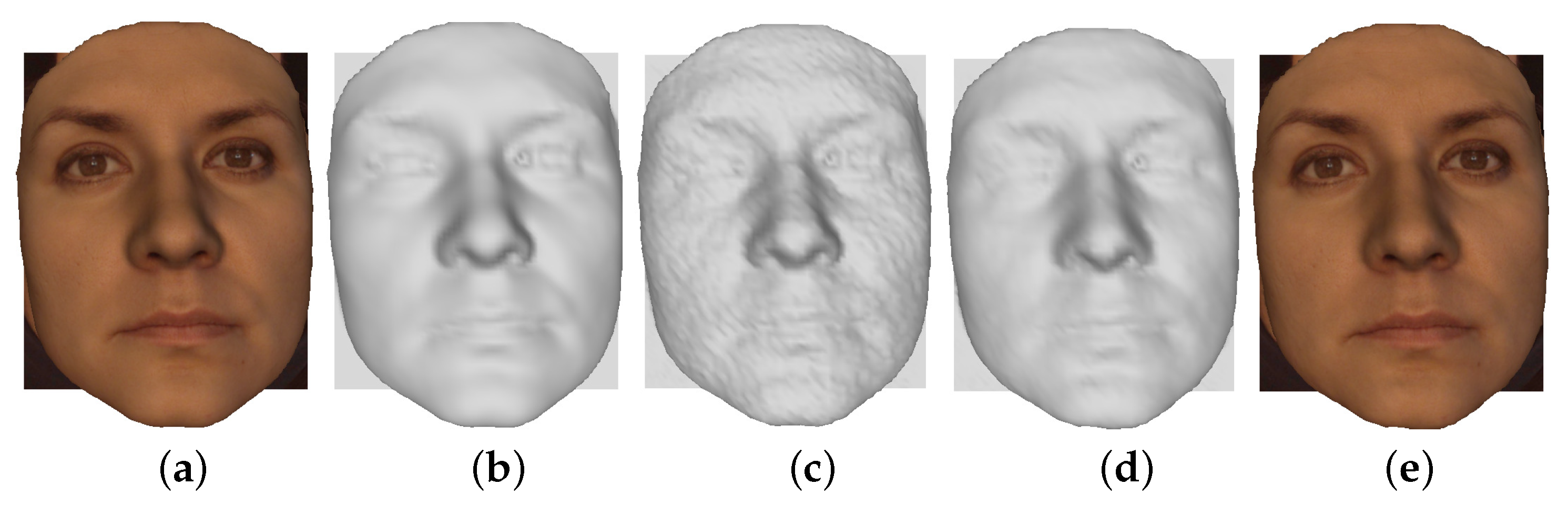
Datasets
5.3. System Evaluation and Discussion
6. Conclusions
Author Contributions
Funding
Institutional Review Board Statement
Informed Consent Statement
Data Availability Statement
Conflicts of Interest
References
- Deng, J.; Guo, J.; Xue, N.; Zafeiriou, S. Arcface: Additive angular margin loss for deep face recognition. In Proceedings of the IEEE/CVF Conference on Computer Vision and Pattern Recognition, Long Beach, CA, USA, 15–20 June 2019; pp. 4690–4699. [Google Scholar]
- Wang, H.; Wang, Y.; Zhou, Z.; Ji, X.; Gong, D.; Zhou, J.; Li, Z.; Liu, W. Cosface: Large margincosine loss for deep face recognition. In Proceedings of the IEEE Conference on Computer Vision and Pattern Recognition, Salt Lake City, UT, USA, 18–23 June 2018; pp. 5265–5274. [Google Scholar]
- Robinson, J.P.; Livitz, G.; Henon, Y.; Qin, C.; Fu, Y.; Timoner, S. Face recognition: Too bias, or not too bias? In Proceedings of the 2020 IEEE/CVF Conference on Computer Vision and Pattern Recognition Workshops (CVPRW), Seattle, WA, USA, 14–19 June 2020; pp. 1–10. [Google Scholar]
- Kosinski, M. Facial recognition technology can expose political orientation from naturalistic facial images. Sci. Rep. 2021, 11, 1–7. [Google Scholar] [CrossRef] [PubMed]
- Medvedev, I.; Shadmand, F.; Cruz, L.; Gonçalves, N. Towards Facial Biometrics for ID Document Validation in Mobile Devices. Appl. Sci. 2021, 11, 6134. [Google Scholar] [CrossRef]
- Wang, Z.; Zhang, X.; Yu, P.; Duan, W.; Zhu, D.; Cao, N. A New Face Recognition Method for Intelligent Security. Appl. Sci. 2020, 10, 852. [Google Scholar] [CrossRef] [Green Version]
- Portrait Quality—Reference Facial Images for MRTD. ICAO. Available online: https://www.icao.int/Security/FAL/TRIP/Documents/TR-PortraitQualityv1.0.pdf (accessed on 25 August 2021).
- Information Technology—Extensible Biometric Data Interchange Formats—Part 5: Face Image Data. ISO/IEC 39794-5:2019. Available online: https://www.iso.org/standard/50867.html (accessed on 25 August 2021).
- Nonis, F.; Dagnes, N.; Marcolin, F.; Vezzetti, E. 3D Approaches and Challenges in Facial Expression Recognition Algorithms—A Literature Review. Appl. Sci. 2019, 9, 3904. [Google Scholar] [CrossRef] [Green Version]
- ID Documents Solutions. Available online: https://jura.hu/travel-id-documents-mrtd-solutions/ (accessed on 15 September 2021).
- Preventing Forgery of Identity Documents. Available online: https://www.idemia.com/lasink/ (accessed on 15 September 2021).
- Security Printing Solutions: Gemalto Surface Features—The Power of a Team. Available online: https://www.gemalto.com/govt/security-features/secure-surface-features/ (accessed on 15 September 2021).
- Dagnes, N.; Vezzetti, E.; Marcolin, F.; Tornincasa, S. Occlusion detection and restoration techniques for 3D face recognition: A literature review. Mach. Vis. Appl. 2018, 29, 789–813. [Google Scholar] [CrossRef]
- Jackson, A.S.; Bulat, A.; Argyriou, V.; Tzimiropoulos, G. Large pose 3d face reconstruction from a single image via direct volumetric cnn regression. In Proceedings of the International Conference on Computer Vision 2017, Venice, Italy, 22–29 October 2017. [Google Scholar]
- Dihl, L.; Cruz, L.; Monteiro, N.; Gonçalves, N. A Content-aware Filtering for RGBD Faces. In Proceedings of the 14th International Joint Conference on Computer Vision, Imaging and Computer Graphics Theory and Applications; SCITEPRESS—Science and Technology Publications: Prague, Czech Republic, 2019; Volume 1, pp. 270–277. [Google Scholar]
- Zollhöfer, M.; Stotko, P.; Görlitz, A.; Theobalt, C.; Nießner, M.; Klein, R.; Kolb, A. State of the Art on 3D Reconstruction with RGB-D Cameras. Comput. Graph. Forum 2018, 37, 625–652. [Google Scholar] [CrossRef]
- Thies, J.; Zollhöfer, M.; Nießner, M.; Valgaerts, L.; Stamminger, M.; Theobalt, C. Real-time expression transfer for facial reenactment. ACM Trans. Graph. 2015, 34, 183:1–183:14. [Google Scholar] [CrossRef]
- Hsieh, P.-L.; Ma, C.; Yu, J.; Li, H. Unconstrained realtime facial performance capture. In Proceedings of the 2015 IEEE Conference on Computer Vision and Pattern Recognition (CVPR), Boston, MA, USA, 7–12 June 2015; pp. 1675–1683. [Google Scholar]
- Bouaziz, S.; Wang, Y.; Pauly, M. Online modeling for realtime facial animation. ACM Trans. Graph. 2013, 32, 1–10. [Google Scholar] [CrossRef]
- Wei, L.-Y.; Lefebvre, S.; Kwatra, V.; Turk, G. State of the art in example-based texture synthesis. In Eurographics 2009, State of the Art Report, EG-STAR; Eurographics Association: Munich, Germany, 2009. [Google Scholar]
- Wei, M.; Huang, J.; Xie, X.; Liu, L.; Wang, J.; Qin, J. Mesh Denoising Guided by Patch Normal Co-Filtering via Kernel Low-Rank Recovery. IEEE Trans. Vis. Comput. Graph. 2019, 25, 2910–2926. [Google Scholar] [CrossRef] [PubMed]
- Taubin, G. A signal processing approach to fair surface design. In SIGGRAPH ’95: Proceedings of the 22nd Annual Conference on Computer Graphics and Interactive Techniques; ACM: New York, NY, USA, 1995; pp. 351–358. [Google Scholar]
- Desbrun, M.; Meyer, M.; Schröder, P.; Barr, A.H. Implicit fairing of irregular meshes using diffusion and curvature flow. In SIGGRAPH ’99: Proceedings of the 26th Annual Conference on Computer Graphics and Interactive Techniques; ACM: New York, NY, USA, 1999; pp. 317–324. [Google Scholar]
- Perona, P.; Malik, J. Scale-space and edge detection using anisotropic diffusion. IEEE Trans. Pattern Anal. Mach. Intell. 1990, 12, 629–639. [Google Scholar] [CrossRef] [Green Version]
- Chia, M.H.; He, C.H.; Lin, H.Y. Novel view image synthesis based on photo-consistent 3D model deformation. Int. J. Comput. Sci. Eng. 2013, 8, 316. [Google Scholar] [CrossRef]
- Lin, H.-Y.; Tsai, C.-L.; Tran, V.L. Depth Measurement Based on Stereo Vision with Integrated Camera Rotation. IEEE Trans. Instrum. Meas. 2021, 70, 1–10. [Google Scholar] [CrossRef]
- Luebke, D. A developer’s survey of polygonal simplification algorithms. IEEE Eng. Med. Boil. Mag. 2001, 21, 24–35. [Google Scholar] [CrossRef]
- Baumgart, B.G. A polyhedron representation for computer vision. In AFIPS ’75: Proceedings of the May 19–22, 1975, National Computer Conference and Exposition; ACM Press: New York, NY, USA, 1975; pp. 589–596. [Google Scholar]
- Wanner, S.; Goldluecke, B. Globally consistent depth labeling of 4d lightfields. In Proceedings of the IEEE Conference on Computer Vision and Pattern Recognition (CVPR), Providence, RI, USA, 16–21 June 2012; pp. 41–48. [Google Scholar]
- Georgiev, T.G.; Lumsdaine, A. Superresolution with Plenoptic 2.0 Cameras. In Frontiers in Optics/Laser Science; The Optical Society: San Jose, CA, USA, 2009; p. STuA6. [Google Scholar]
- Kazemi, V.; Sullivan, J. One millisecond face alignment with an ensemble of regression trees. In Proceedings of the 2014 IEEE Conference on Computer Vision and Pattern Recognition, Columbus, OH, USA, 23–28 June 2014; pp. 1867–1874. [Google Scholar]
- Zhang, Z. Iterative point matching for registration of free-form curves and surfaces. Int. J. Comput. Vis. 1994, 13, 119–152. [Google Scholar] [CrossRef]
- Kovács, P.T.; Balogh, T. 3D visual experience. In High-Quality Visual Experience: Creation, Processing and Interactivity of High-Resolution and High-Dimensional Video Signals; Grgic, M., Kunt, M., Mrak, M., Eds.; Springer: Berlin/Heidelberg, Germany, 2010; pp. 391–410. [Google Scholar]
- Xie, H.; Zhao, X.; Yang, Y.; Bu, J.; Fang, Z.; Yuan, X. Cross-lenticular lens array for full parallax 3-d display with crosstalk reduction. Sci. China Technol. Sci. 2011, 55, 735–742. [Google Scholar] [CrossRef]
- Tao, M.W.; Hadap, S.; Malik, J.; Ramamoorthi, R. Depth from combining defocus and correspondence using light-field cameras. In Proceedings of the 2013 IEEE International Conference on Computer Vision, Sydney, Australia, 2–8 December 2013; pp. 673–680. [Google Scholar]
- Cardoso, J.L.; Goncalves, N.; Wimmer, M. Cost volume refinement for depth prediction. In Proceedings of the 2020 25th International Conference on Pattern Recognition (ICPR), Milan, Italy, 10–15 January 2021; pp. 354–361. [Google Scholar]
- Ferreira, R.; Gonçalves, N. Fast and accurate micro lenses depth maps for multi-focus light field cameras. In German Conference on Pattern Recognition; Springer Science and Business Media LLC: Cham, Switzerland, 2016; pp. 309–319. [Google Scholar]
- Ferreira, R.; Gonçalves, N. Accurate and fast micro lenses depth maps from a 3D point cloud in light field cameras. In Proceedings of the 2016 23rd International Conference on Pattern Recognition (ICPR), Cancun, Mexico, 4–8 December 2016; pp. 1893–1898. [Google Scholar]
- Boyat, A.K.; Joshi, B.K. A Review Paper: Noise Models in Digital Image Processing. Signal Image Process. Int. J. 2015, 6, 63–75. [Google Scholar] [CrossRef]
- Tomasi, C.; Manduchi, R. Bilateral filtering for gray and color images. In Proceedings of the Sixth International Conference on Computer Vision (IEEE Cat. No.98CH36271), Copenhagen, Denmark, 28–31 May 2002. [Google Scholar]
- Lehmann, E.; Casella, G. Theory of Point Estimation; Springer: Berlin/Heidelberg, Germany, 1998. [Google Scholar]
- Savran, A.; Sankur, B. Non-rigid registration based model-free 3D facial expression recognition. Comput. Vis. Image Underst. 2017, 162, 146–165. [Google Scholar] [CrossRef]
- Sony: Sony Depthsensing Solutions. 2019. Available online: https://www.sony-depthsensing.com/ (accessed on 15 September 2021).


| Noise level | Bilateral | Gaussian | Ours |
|---|---|---|---|
| 0.0 | 0.6615 | 1.8459 | 0.4859 |
| 0.5 | 0.6782 | 1.8484 | 0.4991 |
| 0.7 | 0.6970 | 1.8595 | 0.5289 |
| 1.0 | 0.7117 | 1.8819 | 0.5383 |
| 2.0 | 0.8236 | 1.9450 | 0.7218 |
Publisher’s Note: MDPI stays neutral with regard to jurisdictional claims in published maps and institutional affiliations. |
© 2021 by the authors. Licensee MDPI, Basel, Switzerland. This article is an open access article distributed under the terms and conditions of the Creative Commons Attribution (CC BY) license (https://creativecommons.org/licenses/by/4.0/).
Share and Cite
Dihl, L.; Cruz, L.; Gonçalves, N. Card3DFace—An Application to Enhance 3D Visual Validation in ID Cards and Travel Documents. Appl. Sci. 2021, 11, 8821. https://doi.org/10.3390/app11198821
Dihl L, Cruz L, Gonçalves N. Card3DFace—An Application to Enhance 3D Visual Validation in ID Cards and Travel Documents. Applied Sciences. 2021; 11(19):8821. https://doi.org/10.3390/app11198821
Chicago/Turabian StyleDihl, Leandro, Leandro Cruz, and Nuno Gonçalves. 2021. "Card3DFace—An Application to Enhance 3D Visual Validation in ID Cards and Travel Documents" Applied Sciences 11, no. 19: 8821. https://doi.org/10.3390/app11198821
APA StyleDihl, L., Cruz, L., & Gonçalves, N. (2021). Card3DFace—An Application to Enhance 3D Visual Validation in ID Cards and Travel Documents. Applied Sciences, 11(19), 8821. https://doi.org/10.3390/app11198821