Using Artificial Neural Network Algorithm and Remote Sensing Vegetation Index Improves the Accuracy of the Penman-Monteith Equation to Estimate Cropland Evapotranspiration

Abstract

Accurate estimation of evapotranspiration (ET) can provide useful information for water management and sustainable agricultural development. However, most of the existing studies used physical models, which are not accurate enough due to our limited ability to represent the ET process accurately or rarely focused on cropland. In this study, we trained two models of estimating croplands ET. The first is Medlyn-Penman-Monteith (Medlyn-PM) model. It uses artificial neural network (ANN)-derived gross primary production along with Medlyn’s stomatal conductance to compute surface conductance (Gs), and the computed Gs is used to estimate ET using the PM equation. The second model, termed ANN-PM, directly uses ANN to construct Gs and simulate ET using the PM equation. The results showed that the two models can reasonably reproduce ET with ANN-PM showing a better performance, as indicated by the lower error and higher determination coefficients. The results also showed that the performances of ANN-PM without the facilitation of any remote sensing (RS) factors degraded significantly compared to the versions that used RS factors. We also evidenced that ANN-PM can reasonably characterize the time-series changes of ET at sites having a dry climate. The ANN-PM method can reasonably estimate the ET of croplands under different environmental conditions.

1. Introduction

Evapotranspiration (ET) is the process by which vegetation and groundwater transport water vapor to the atmosphere, mainly including plant transpiration and soil evaporation [1], with transpiration being dominant on a global scale [2]. Estimation of ET is an important basis for reasonable irrigation over croplands at a regional scale [3]; at the same time, as an important part of energy balance and the water cycle, ET also affects atmospheric circulation and plays an important role in regulating climate. Cropland is an important ecosystem on the land surface. Thus, the accurate estimation of cropland ET is of great significance for the rational irrigation of crops and the study of material and energy balance under the background of climate change [4].

The Penman-Monteith (PM) equation is the most commonly used framework for estimating regional or global ET. The regional-scale modeling process based on the PM equation is a simulation of surface conductance (Gs), and this parameter accounts for the largest source of uncertainty in ET modeling based on the PM equation on a regional scale. Cleugh et al. [5] tested two models of estimating land surface evaporation, the surface energy balance model and PM-based approach using remote sensing (RS)-derived leaf area index (LAI), to estimate Gs at two Australian flux stations, and the PM-based method proved better. Mu et al. [6] found that the surface conductivity model of Cleugh et al. [5] was unreliable when used to estimate the global ET of 19 AmeriFlux sites due to the oversimplified estimates of surface conductance. Therefore, the canopy conductance and ET algorithms based on the PM method of Cleugh et al. [5] were improved by using the RS and global meteorological data. The algorithm of Mu et al. [6] considered the surface energy partitioning process and the environmental constraints of ET, but the performance of Mu et al. [6] still remains uncertain. Mu et al. [7] further improved the global terrestrial ET algorithm and showed the improved algorithm performed better compared to the original. Based on Cleugh et al. [5] and Mu et al. [6], Leuning et al. [8] developed a biophysical model to estimate Gs and introduced a simpler soil evaporation algorithm than the MOD16 algorithm [6] to calculate daily average evaporation. The results showed that the PM equation, incorporated with the RS leaf area index, could more reliably estimate the evaporation rate. However, the performances of the model degraded if a fixed value of maximum stomatal conductance (g_sx) was used to estimate the surface conductance across a wide range of vegetation categories [8]. Zhang et al. [9] further developed the Gs formula and calculated the land surface ET at a spatial resolution of 0.05 ° using the PM equation. Yebra et al. [10] reversed the PM equation to obtain the Gs of the plant canopy, and then the estimated Gs was used to retrieve actual ET using the parameterized PM equation. Kitao et al. [11] also applied a semi-empirical model dependent on photosynthesis [12] to estimate canopy Gs. Because the method of Ball et al. [12] restricted the applicability of the model, Yan et al. [13] used a simple biophysical model to calculate Gs, and then the computed Gs was used to calculated global ET based on the PM equation. Mallick et al. [14] estimated Gs by integrating the radiometric surface temperature into a combined structure of the PM model and the Shuttleworth–Wallace model and used the simplified surface energy balance model to estimate ET. The method of Yan et al. [13] used the leaf area index and surface meteorological data, while Mallick et al. [14] did not use any leaf-scale empirical parameter model to determine Gs and ET. However, the method of Mallick et al. [14] had a tendency to overestimate Gs. For areas with limited data, the method of Mallick et al. [14] was considered to be further improved. Therefore, Bhattarai et al. [15] used RS and reanalysis data to develop an automatic multi-model to estimate regional ET in important areas.

In order to reduce the uncertainties in ET estimation due to the difficulty in estimating Gs, semi-empirical models that use machine learning (ML) to more accurately calculate the Gs in the PM equation were proposed [16,17,18]. For example, Zhang et al. [18] combined ML, in which only temperature (Ta) data was used with the PM equation to estimate crop ET, and showed that the accuracy of the ML-based PM approach was better than the Hargreaves (HARG) method. However, the computational complexity of the model of Zhang et al. [18] is relatively high and requires more storage space. Traore et al. [17] evaluated different ML methods based on only temperature data to calculate ET under the framework of the PM equation. The determination coefficients (R²) were significantly increased when wind speed data was added to the model of [17]. Thus, only one meteorological input is not enough for reasonably quantifying ET. Multiple data combinations can effectively improve the accuracy of the ET model. Zhao et al. [19] developed a hybrid model to estimate latent heat flux based on various variables (such as soil moisture, carbon dioxide concentration (Ca), etc.), combining ML models with the PM method. The results showed that the hybrid model is more adaptable to extreme environments compared with the pure ML method. Due to a lack of reliable and spatiotemporal continuous soil moisture data sets on a global scale, the model of Zhao et al. [19] is limited to a regional scale and cannot be applied on a global scale. Therefore, using only a single datum or a data set that is difficult to obtain will limit the application of the model on a regional or global scale. Therefore, we use a variety of globally available data combined with ML methods in order to improve the estimates of ET over croplands. The ML approaches can represent the complex and non-linearly relationships between inputs and the target [20], and assess the adaptivity of multiple ET models of different environments [21], with smaller errors under a specific environmental condition.

Nowadays, most of the existing studies on estimating ET use physical models [22,23,24,25] or purely rely on ML algorithms [26,27,28,29,30,31]; these methods are not accurate enough to represent the ET due to the limited ability to understand the ET process. The hybrid ET model that combines the physical framework, namely the PM equation, and ML algorithms has proved to be effective in ET estimates [19,32]. The ML approaches resolved the difficulty of characterizing the complex environmental constraints on ET in the hybrid model, while the PM framework ensures the model’s robustness. It is worth noting that the pure ML models may yield comparable or even better performance compared to the hybrid model [19] or individual physical models [26,33]. However, without physical constraints, the reliability of the pure ML models depends on the representativeness of training data [33]. As a result, the pure ML models are vulnerable to extreme environmental conditions [19], while the hybrid models show more robust performances under these conditions [19].

In this study, we aim to improve the estimates of cropland ET by training a hybrid ET model based on an artificial neural network (ANN) and PM equation, investigate whether the use of RS factors can improve the performances of hybrid models, and evaluate the ANN-PM model to simulate ET on a daily scale over flux sites covering a wide range of climate dryness.

2. Material and Methods

The research flow chart of this study is shown in Figure 1. We trained two methods to estimate ET. First, the Gs model is constructed using meteorological data and remote sensing data, and subsequently, used to simulate ET under the framework of the PM equation. Secondly, Gs is estimated using ANN-derived GPP in conjunction with Medlyn stomatal conductance, and then the computed Gs is used to estimate ET using the PM equation.

2.1. Material

The meteorological data used in this study were retrieved from the meteorological observation data of the eddy covariance flux tower at 17 flux sites. Figure 2 shows the map representation of the 17 flux sites of cropland over the globe.

The information of the 17 flux sites is shown in

Table 1. Description of flux sites.

Site Code	Latitude	Longitude	Mean Annual Temperature (°C)	Mean Annual Precipitation (mm)	Years	Reference
BE-Lon	50.55	4.75	11.41	766.50	2004–2014	Moureaux et al. [35]
CH-Oe2	47.29	7.73	9.56	2062.25	2004–2014	Moors et al. [36]
DE-Geb	51.10	10.91	9.67	532.90	2001–2014	Anthoni et al. [37]
DE-Kli	50.89	13.52	7.77	810.30	2004–2014	Brust et al. [38]
DE-RuS	50.86	6.45	10.80	551.15	2011–2014	Eder et al. [39]
DE-Seh	50.87	6.45	10.29	573.05	2007–2010	Korres et al. [40]
FR-Gri	48.84	1.95	10.96	598.60	2004–2014	Loubet et al. [41]
IT-BCi	40.52	14.96	17.88	1197.20	2004–2014	Ranucci et al. [42]
IT-CA2	42.38	12.03	14.84	766.50	2011–2014
US-ARM	36.60	−97.49	15.27	646.05	2003–2012	Raz-Yaseef et al. [43]
US-CRT	41.63	−83.35	10.85	810.30	2011–2013	Chu et al. [44]
US-Ne1	41.1651	−96.477	10.54	846.80	2001–2013	Verma et al. [45]
US-Ne2	41.1649	−96.470	10.26	876.00	2001–2013	Suyker and Verma [46]
US-Ne3	41.1797	−96.440	10.38	697.15	2001–2013	Suyker and Verma [46]
US-Tw2	38.1047	−121.643	15.23	386.90	2012–2013	Knox et al. [47]
US-Tw3	38.1159	−121.647	16.00	343.10	2013–2014	Baldocchi et al. [48]
US-Twt	38.1087	−121.653	14.75	357.70	2009–2014	Hatala et al. [49]

. The 17 flux sites of cropland over the globe were located in different countries (such as Germany, the United States, France, and Italy). DE-Kli and IT-BCi have the lowest (7.77 °C) and highest (17.88 °C) mean annual temperatures, respectively. The annual precipitation of these sites varies from 343.1 (US-Tw3) to 2062.25 mm (CH-Oe2). We divide the flux data set into the training set, validation set, and test set, the ratios of which are 60%, 20%, and 20%, respectively, and the three datasets are used to train, validate, and test the ANN model. The vegetation index and reflectance data were retrieved from MODIS MOD09A1 (https://modis.ornl.gov/data.html, accessed on 27 February 2020), having a spatial resolution of 500 m. These flux data and MODIS data were used to training the two models of estimating ET. The time series of MODIS data were extracted according to the longitude and latitude coordinates of the flux sites. The spectral index was calculated using the MOD43A4 product, following the formulations shown in

Table 2. Calculation of vegetation index. rx represents the reflectivity of MODIS bands (x = 1–7), NDVI is the normalized difference vegetation index, NIRv is near-infrared reflectance of vegetation.

Index	Formula
NDVI	$\mathrm{NDVI}=\frac{r2-r1}{r2+r1}$
NIRv	$\mathrm{NIRv}=\mathrm{NDVI}\ast r2$

. NDVI is usually used to reflect the information of vegetation coverage and growth. In order to obtain information on a larger regional scale, a new vegetation index NIRv is introduced [19], which can reflect the photosynthetic capacity of surface vegetation better. NIRv is the product of the total near-infrared reflectance (NIRt) (MODIS second band) and NDVI. NIRv is a remote sensing measurement of canopy structure, which can more accurately predict photosynthesis [34]. The shortwave infrared band (SWIR) is usually used to reflect water stress and is calculated by using the reflectance data directly.

2.2. Two ET Models Based on ANN

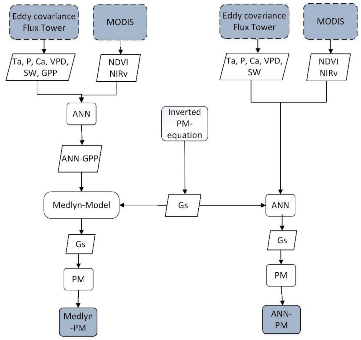
In this study, two models were trained based on the PM equation, and the difference lies in the Gs calculation. The following two summaries introduce the two methods in detail. The formula of the PM equation is as follows:

$$\lambda \mathrm{E}=\frac{\left(Rn-G\right)·\mathrm{\Delta }+\rho ·Cp·D·Ga}{\mathrm{\Delta }+\gamma \left(1+Ga/Gs\right)}$$

(1)

where $\lambda \mathrm{E}$ is evapotranspiration, Rn is net radiation, G is soil heat flux, Δ is the gradient of the saturation vapor pressure versus atmospheric temperature, ρ is air density, Cp is the specific heat at constant pressure of air, D is the vapor pressure deficit of the air, Ga is the aerodynamic conductance, and γ is the psychometric constant.

In order to test the effects on the accuracy of using different combinations of input variables, different combinations of input variables in the ANN are shown in

Table 3. Different combinations of input variables in the ANN. Ta is temperature, P is precipitation, SW is solar radiation, Ca is carbon dioxide concentration, VPD is vapor pressure deficit, NDVI is normalized difference vegetation index, NIRv is near-infrared reflectance of vegetation, and SWIR is shortwave infrared band.

Number	Input Parameters
1	Ta, P, SW, Ca, VPD
2	Ta, P, SW, Ca, VPD, NDVI
3	Ta, P, SW, Ca, VPD, NDVI, NIRv
4	Ta, P, SW, Ca, VPD, NDVI, NIRv, SWIR

.

2.2.1. ANN-PM Model

We trained an ANN-PM model based on ANN and PM equations to estimate ET. ANN is a commonly used ML method, which has been widely used in estimating ET. It consists of a large number of nodes, called neurons, which are connected to each other. The typical structure of ANN used to estimate ET is shown in Figure 3.

ANN contains three layers: the input layer, hidden layer, and output layer. The input layer is responsible for receiving input data, the hidden layer constructs the relationships between the input and output, and the output layer outputs the predicted target values. The variables input to ANN in this study includes Ta, precipitation (P), solar radiation (SW), Ca, vapor pressure deficit (VPD), normalized difference vegetation index (NDVI), and near-infrared reflectance of vegetation (NIRv). In the variables we used, Ta, SW, Ca, and VPD can affect canopy conductivity from different aspects [50]. The consideration of P is mainly to represent the influence of canopy interception on ET. Thus they are selected to model Gs. There is an interaction and mutual influence between the transpiration and photosynthetic capacity of plants, and ET is dominated by transpiration. The vegetation index, NIRv, is considered in order to better reflect the impact of the photosynthetic capacity of the surface vegetation on evapotranspiration. NIRv is able to characterize seasonable variations in canopy scale photosynthesis rate without additional environmental factors that are conventionally used to constrain photosynthesis [34]. These variables are used to train ANN to the Gs model. Referring to Zhao et al. [19], we used the ANN model to model ln(Gs) rather than Gs because the logarithmic form can effectively reduce the effect of errors in Gs calculated from the observations. Finally, the logarithm of Gs obtained by ANN simulation is converted to Gs, and then the converted Gs is input into the PM equation to calculate ET. Here, Gs values used to train the ANN model were calculated from the observed ET along with the inverted PM equation [51]. In order to avoid over-fitting, the network model is repeatedly trained, where the number of hidden layers ranges from 1 to 10, and the number of neurons in each layer increases from 1 to 128, with an interval of 8. Then, we choose the optimal ANN structure as the best model.

2.2.2. Medlyn-PM Model

The Medlyn-PM model uses ANN-derived GPP in conjunction with a theoretical Gs model to estimate surface conductance, and then the computed Gs is used to estimate ET using the PM equation. Firstly, we use the optimal ANN structure selected above to train the GPP model. Secondly, on the pixel scale, the computed GPP, Ca, and air vapor pressure deficit are used for Gs regression analysis to establish the relationship among them and determine the undetermined coefficients g₀ and g₁. Then, we use the above variables and the relationship between them to build the Gs model. Finally, the constructed Gs is input into the PM equation to calculate ET. The relationship is as follows [52]:

$$Gs=1.6\ast \frac{\mathrm{GPP}}{\mathrm{Ca}}\ast \left(\frac{g_1}{\sqrt{\mathrm{D}}}+1\right)+g_0$$

(2)

where Gs is stomatal conductance, GPP is gross primary production, Ca is CO₂ concentration of the air, g₁ and g₀ are undetermined coefficients derived from regression analysis, and D is the vapor pressure deficit of the air. The minimum value of D is fixed to 0.1 KPa.

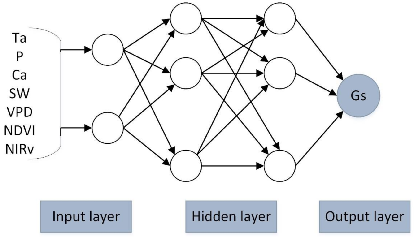
2.3. ANN Architecture Optimization

The ML method, i.e., ANN, used in the ANN-PM and the Medlyn-PM, considers input variables, including Ta, P, SW, Ca, VPD, NIRv, and NDVI. Usually, in order to reduce over-fitting, the network model is repeatedly trained. Thus, we need to recognize the best ANN structure. In our study, the optimal ANN is determined in terms of mean square error (MSE) while minimizing the number of degrees of freedom based on the Akaike Information Criterion (AIC). AIC is a standard to measure the goodness of fit of the statistical model. AIC encourages the goodness of data fitting but tries to avoid over-fitting. Therefore, the priority model should be the one with the lowest AIC value. Cropland ET is estimated by combining the predictive output of ANN with the PM equation. The calculation formula of the AIC indicator is as follows [53]:

$$\mathrm{AIC}=\log \left(\mathrm{MSE}\right)+\frac{2q}{n}$$

(3)

where MSE is mean square error, q is the total number of parameters in the network, and n is the number of observations in the training sample.

2.4. Model Evaluation

2.4.1. Model Performance Measurement

The model performance evaluation metrics used in the study include root mean square error (RMSE), mean absolute error (MAE), and determination coefficients (R²). The calculations of these metrics are shown in

Table 4. Calculation formula of evaluation parameters. RMSE is the root mean square error, MAE is the mean absolute error, and R² is the determination coefficients. fi: Predicted value: $\overline{fi}$ Mean value of the predicted values; yi: Experiment value;$\overline{yi}$: Mean value of the observed values; m: Total amount of experimental data.

Evaluation Parameters	Formula
RMSE	$\sqrt{\frac{{{\displaystyle \sum }}_{i=1}^m{\left(fi-yi\right)}^2}{m}}$
MAE	$\frac{{{\displaystyle \sum }}_{i=1}^m\left|fi-yi\right|}{m}$
R2	${\left(\frac{{{\displaystyle \sum }}_{i=1}^m\left(yi-\overline{yi}\right)\left(fi-\overline{fi}\right)}{\sqrt{{{\displaystyle \sum }}_{i=1}^m{\left(yi-\overline{yi}\right)}^2}\sqrt{{{\displaystyle \sum }}_{i=1}^m{\left(fi-\overline{fi}\right)}^2}}\right)}^2$

.

RMSE is the standard deviation between the predicted and true values, reflecting the degree that the predicted values explain the true values [54]. MAE is the mean error of evaluating a set of predictions and is the average value of the absolute difference between predicted and experimental values on test samples, but MAE is less sensitive to extreme values than RMSE [55]. R² is determined by drawing a scatter plot between the observed and predicted value. Lower RMSE, MAE, and higher R² correspond to a better performance of the model.

2.4.2. Evaluating the Model Used to Estimate ET under Dry Climate

Modeling ET in dry regions is more challenging than in other regions, especially for croplands. Because the water status of croplands is affected by irrigation, and the information of irrigation on a regional scale is difficult to obtain. On the other hand, in arid areas, most of the precipitation is consumed in the process of ET, and inadequate water supply could substantially limit the growth of crops in these regions. Therefore, accurate estimation of ET plays an important role in the sustainable development of agriculture in arid areas. Research on modeling ET in dry climates can facilitate rational cropland irrigation, maintaining stable crop production in dry regions.

We analyzed the performance of the models we trained in estimating ET under a dry climate. The aridity index (AI) is a means and tool to determine the drought degree and range of a certain period quantitatively, and it is also an indicator of the degree of dry and wet in a region. The calculation formula of the AI is as follows [56]:

$$\mathrm{AI}=\frac{\mathrm{P}}{\mathrm{PET}}$$

(4)

where AI is aridity index, PET is potential evapotranspiration, and P is the average precipitation. The AI calculation of each site is limited to the time range covered by the site. Low AI corresponds to a dry climate. We selected the sites with the AI values below 0.5 as arid areas by calculating the AI values of each flux site.

3. Results

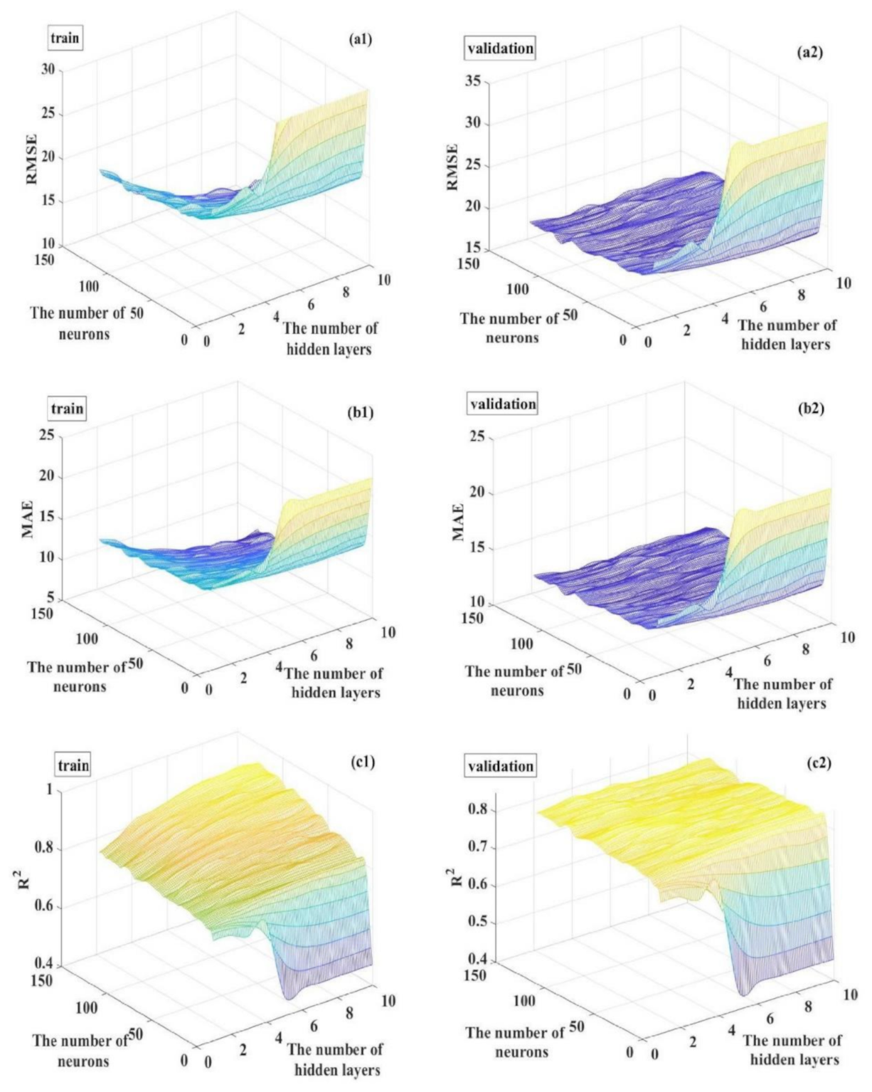
3.1. Model Parameter Optimization

The undetermined parameters g₀ and g₁ were required for running Medlyn-PM. They were determined by fitting the analytical Gs equation, $Gs=1.6\ast \frac{\mathrm{GPP}}{\mathrm{Ca}}\ast \left(\frac{g_1}{\sqrt{\mathrm{D}}}+1\right)+g_0$, and we obtained that g₀ = 0.06 and g₁ = 3.94. The variations in RMSE/MAE/R² with the change of the numbers of hidden layers and neurons for the ANN-PM model with training and validation datasets are presented in Figure 4.

The figure shows that the RMSE and MAE of ANN-PM with the training dataset decrease gradually as the number of hidden layers (HL) and the number of neurons increase. The RMSE and MAE of ANN-PM with the validation dataset decrease as the numbers of hidden layers (HL) and neurons increase from 1 (the number of HL) −1 (the number of neurons) to 10–48 but increase after the number of the two parameters become larger than 1–48. As the number of hidden layers and the number of neurons increase to 10–128, the R² of the training dataset reaches a maximum value (0.94), and the R² of the validation dataset is concentrated around 0.80. Then, considering the AIC values, we identified the best architectures of ANN-PM (AIC = −0.76) and Medlyn-PM (AIC = −0.55) models and the key parameters are shown in

Table 5. The key parameters of the two models. ANN is artificial neural network and PM is the Penman-Monteith.

	ANN-PM Model	Medlyn-PM Model
The number of hidden layers	2	2
The number of neurons	48	1

. The ANN-PM model has an ANN structure with two hidden layers and 48 neurons in each layer. The AIC index is also used to select the ANN-based GPP model in Medlyn-PM, and the optimal model has two hidden layers and one neuron in each layer.

Figure 4. A three-dimensional graph between the number of hidden layers, the number of neurons, and RMSE/MAE/R² of the training and validation datasets of the ANN-PM model. (a1) is the RMSE of the training, (a2) is the RMSE of the validation, (b1) is the MAE of the training, (b2) is the MAE of the validation, (c1) is the R² of the training, (c2) is the R² of the validation. RMSE is the root mean square error, MAE is the mean absolute error, and R² is the determination coefficient.

Figure 4. A three-dimensional graph between the number of hidden layers, the number of neurons, and RMSE/MAE/R² of the training and validation datasets of the ANN-PM model. (a1) is the RMSE of the training, (a2) is the RMSE of the validation, (b1) is the MAE of the training, (b2) is the MAE of the validation, (c1) is the R² of the training, (c2) is the R² of the validation. RMSE is the root mean square error, MAE is the mean absolute error, and R² is the determination coefficient.

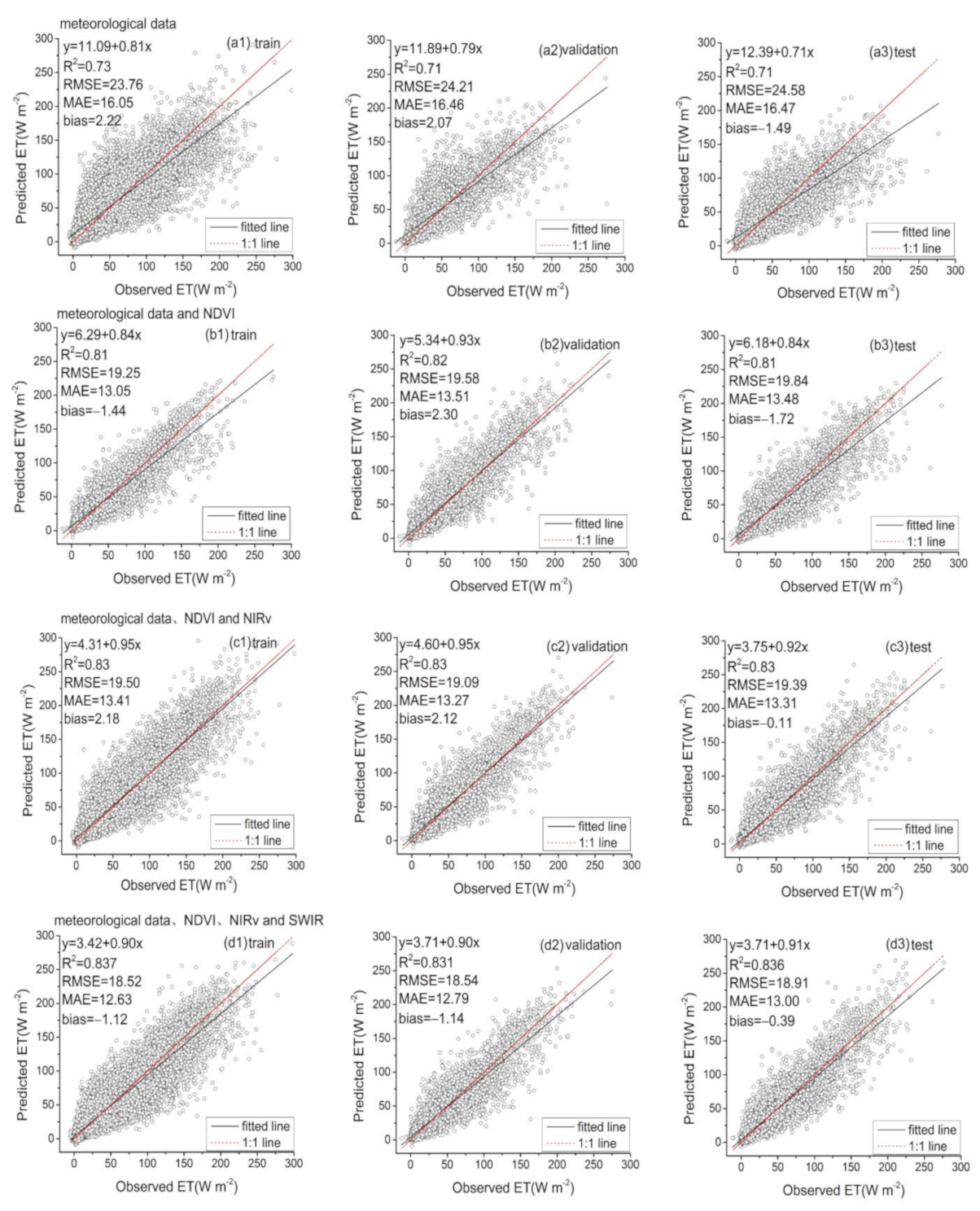
3.2. Comparison of ANN Model with Different Input Data

The input data of ANN in the ANN-PM model includes meteorological data (Ta, P, SW, Ca, and VPD) and remote sensing data (NIRv and NDVI). We investigate the accuracy of estimating ET using the optimized ANN-PM (two hidden layers and 48 neurons in each layer) with several combinations of input data (Table 3). Figure 5 shows the comparisons between the predicted ET values and the measured values of cropland ET in the training, validation, and test datasets across all flux sites.

As shown in Figure 5, all the employed models provide different accuracies under different input combinations. The accuracy of predicted ET values differs significantly depending on the model types and input combinations. Except for the second input combination, all input combinations show the highest R² in the training stage (Figure 5(a1,c1,d1)). The ranks of the input combinations under investigation in terms of prediction accuracy are (the value in parentheses after RMSE indicates the percentage of RMSE relative to the observed value): the fourth input combination (R² = 0.831–0.837, RMSE = 18.52–18.91 W m⁻² (38.42–38.86%), MAE = 12.63–13.00 W m⁻²), the third input combination (R² = 0.83, RMSE = 19.09–19.50 W m⁻² (39.84–40.46%), MAE = 13.27–13.41 W m⁻²), the second input combination (R² = 0.81–0.82, RMSE = 19.25–19.84 W m⁻² (39.94–41.05%), MAE = 13.05–13.51 W m⁻²), and the first input combination (R² = 0.71–0.73, RMSE = 23.76–24.58 W m⁻² (49.29–50.75%), MAE = 16.05–16.47 W m⁻²). In the testing stage, the models of the third input combination and fourth input combination have identical performance in estimating ET, both of which performed superior to the second input combination and the first input combination in predicting ET. These results confirm that the model using all input variables (meteorological data and three remote sensing data factors (NDVI, NIRv, SWIR)) achieves the best performances (RMSE = 18.52–18.91 W m⁻² (38.42–38.86%), MAE = 12.63–13.00 W m⁻², and R² = 0.831–0.837) compared with those using a subset of all the variables. However, the model using meteorological data and two remote sensing data factors (NDVI and NIRv) is also capable of predicting ET with acceptable accuracy, having the RMSE and MAE values of 19.09–19.50 W m⁻² (39.84–40.46%) and 13.27–13.41 W m⁻², respectively. When using only meteorological data, the model shows degraded performance with larger errors (RMSE = 23.76–24.58 W m⁻² (49.29–50.75%) and MAE = 16.05–16.47 W m⁻²) and smaller determination coefficients (R² = 0.71–0.73). The model using the combination of meteorological data and one remote sensing factor, NDVI, shows intermediate results (RMSE = 19.25–19.84 W m⁻² (39.94–41.05%), MAE = 13.05–13.51 W m⁻², and R² = 0.81–0.82). The model using meteorological data and three remote sensing data factors (NDVI, NIRv, and SWIR) showed comparable performance with that using meteorological data and two remote sensing data factors (NDVI, NIRv). Therefore, it can be concluded that remote sensing data in the ANN model facilitated the improvement of the estimates of croplands ET.

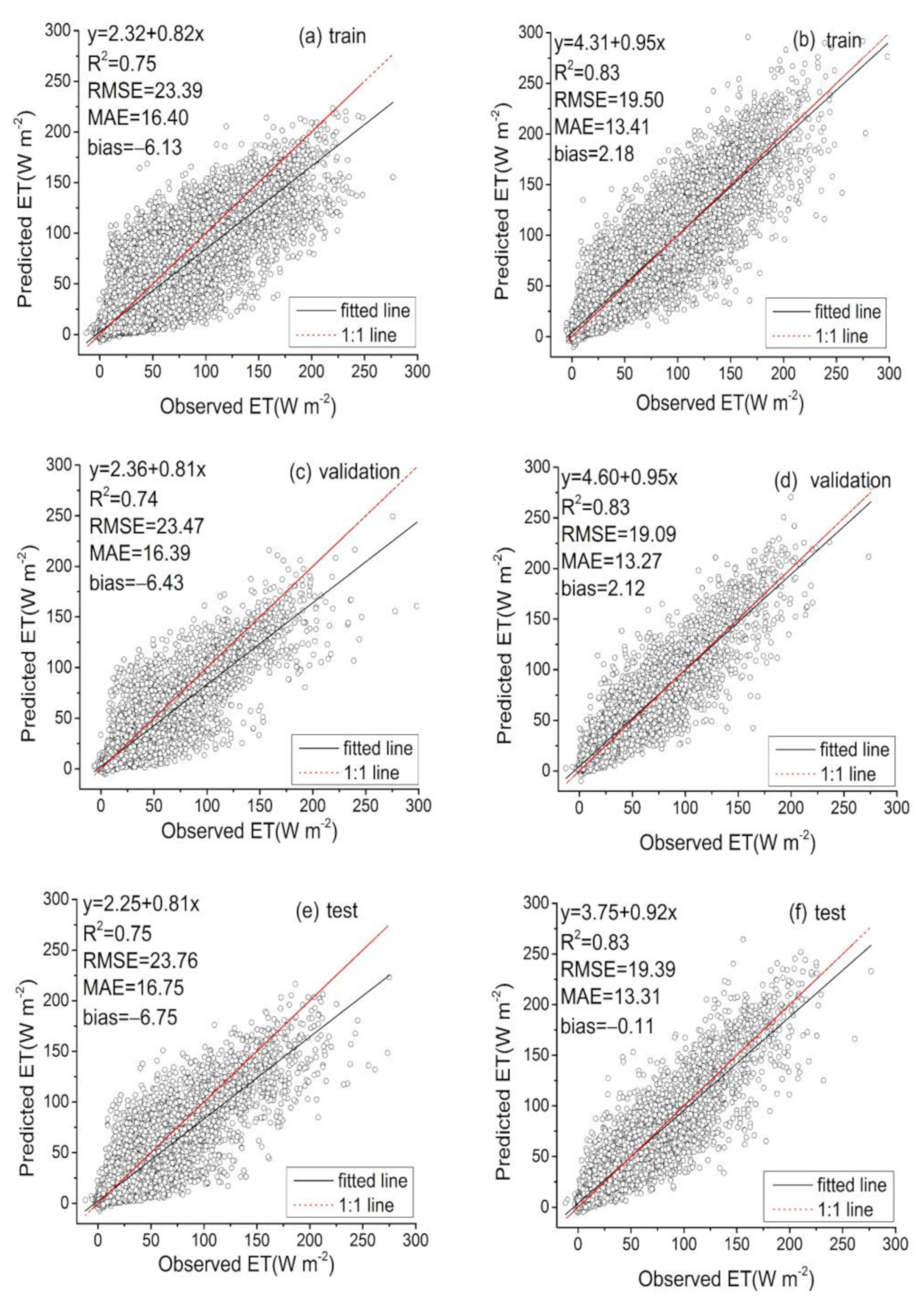
3.3. Comparison of ANN-PM and Medlyn-PM

Figure 6 shows the scatter plots of measured ET vs. predicted ET by the Medlyn-PM and the ANN-PM model, respectively. At the site scale, the two models differ substantially in performance from each other. Figure 6 shows good correlations between the observed ET and the predicted ET by the two methods (R² = 0.75 and 0.83). Figure 6 also illustrates that the R² value of the ANN-PM model is 0.08–0.09 higher than that of the Medlyn-PM model and the RMSE and MAE of ANN-PM are 4.26–4.3 and 3.12–3.34 W m⁻² smaller than that of the Medlyn-PM model, respectively. Overall, the ANN-PM model shows relatively high accuracy with smaller RMSE and MAE, and larger R² (RMSE = 19.09-19.50 W m⁻² (39.84–40.46%), MAE = 13.27–13.41 W m⁻², R² = 0.83) in estimating cropland ET compared to the Medlyn-PM model (RMSE = 23.39–23.76 W m⁻² (49.95–51.14%), MAE = 16.39–16.75 W m⁻², and R² = 0.74–0.75), indicating a great advantage in estimating cropland ET using the ANN-PM model.

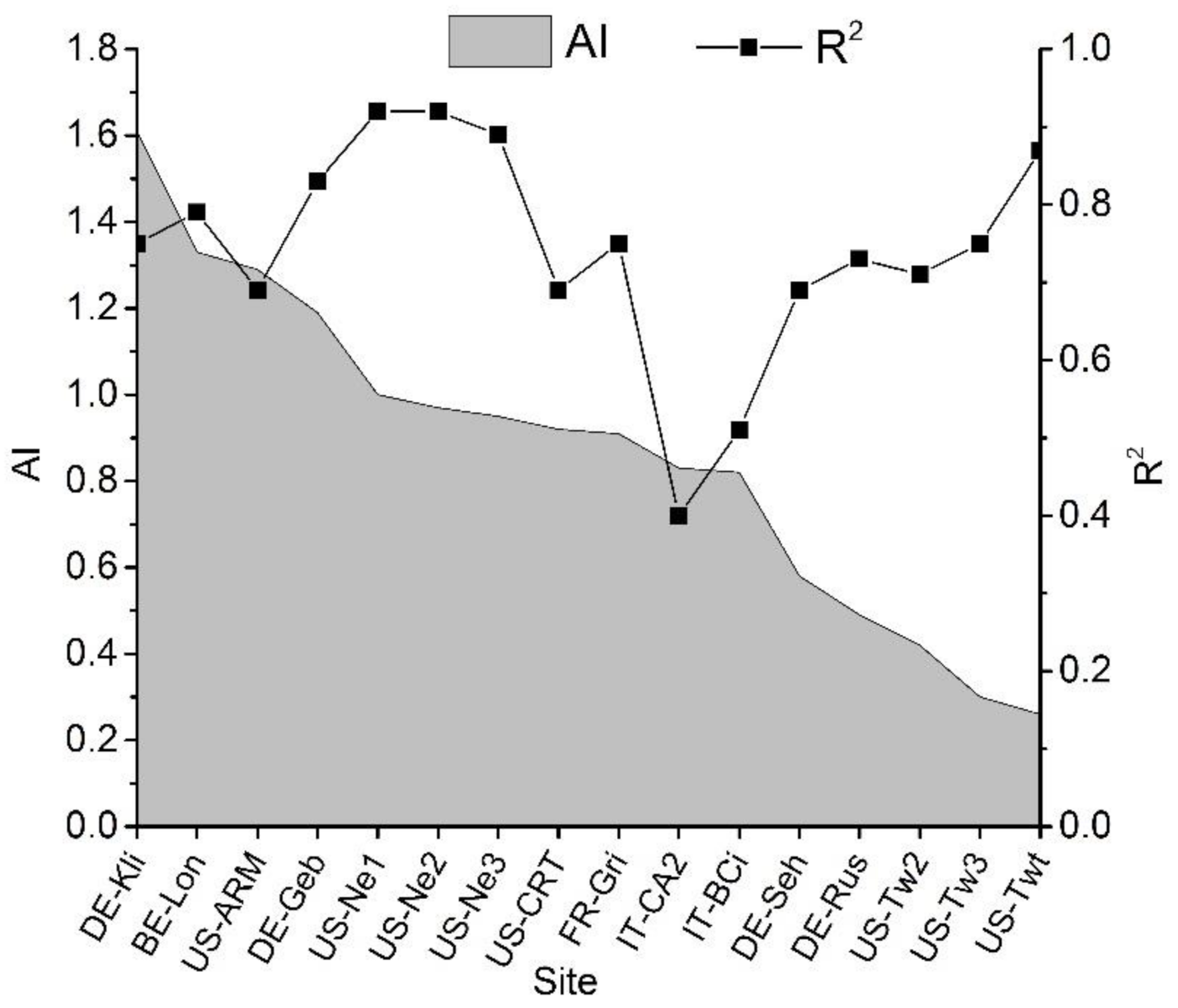
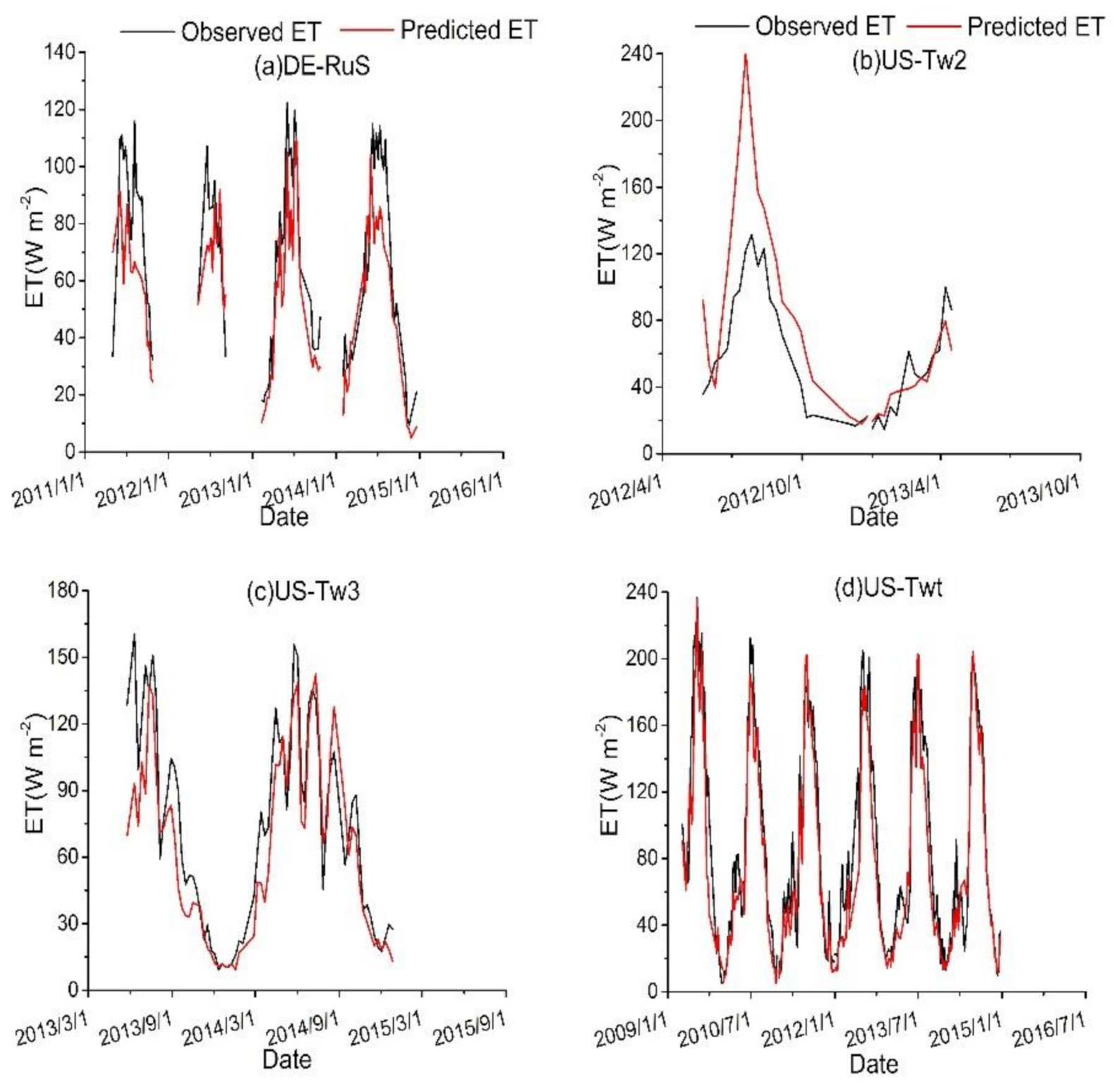
3.4. Accuracy of ANN-PM Model under Dry Climates

In arid areas, most of the precipitation is consumed in the process of ET, and inadequate water supply could substantially limit the growth of crops in these regions. Therefore, accurate estimation of ET plays an important role in the sustainable development of agriculture in arid areas. Hence, we evaluated the ANN-PM model to simulate ET on a daily scale over flux sites covering a wide range of climate dryness, measured using aridity index (AI). The R² between simulation and observation is used to measure the model performance. The variations in R² of each flux site in relation to site-scale AI are shown in Figure 7, where low AI values correspond to dry climates. The driest site is US-Twt, followed by US-Tw3, US-Tw2, and DE-Rus. The average R² of the 16 flux sites is 0.74, and the average R² of the driest four flux sites with an AI index lower than 0.5 (DE-Rus = 0.49, US-Tw2 = 0.42, US-Tw3 = 0.30, and US-Twt = 0.26) is 0.77. In terms of R², the performances of the ANN-PM model at the dry sites are reasonable and comparable to those at the wet sites (Figure 7).

The ANN-PM model can capture the time-series changes of ET at the dry sites well (Figure 8, four sites with an AI index lower than 0.5). At the driest site, US-Twt, which is a paddy field site, ET predicted by the ANN-PM model agreed well with the observations, indicating that the model can reflect the influence of irrigation on cropland ET under dry conditions. Consequently, the ANN-PM model can simulate cropland ET across a wide range of gradients of climate dryness, showing great potential to estimate cropland ET accurately on a regional scale.

4. Discussion

4.1. Discussion of the Number of Sites

We used 17 sites in our study, and the time span of all sites is 2001–2014 (Table 1). The entire dataset contains more than 50,000 samples on a daily scale, which are large enough for establishing the ML-based method. As we know, the size of the sample we used is larger than some existing publications. For example, Zhu et al. [31] used nine stations in the arid region of Northwest China during the period 2002–2016. Yin et al. [57] evaluated ET in the eddy covariance flux observations at 14 Chinese flux tower sites during the period 2003–2017, and each site has at least 3 years of reliable data. Hossein Kazemi et al. [58] only used the daily meteorological records of seven weather stations in Iran for 10 years (2008–2017). Therefore, our data are enough to train a machine learning model. Our study is mainly for cropland. There are currently limited open-access cropland sites, but our sites cover the current main farming areas. These areas cover different climate types. Therefore, our model has wide applicability. There is currently a lack of stations in tropical regions. When applied in this climate region, the model needs to be further tested.

4.2. Comparison between this Research and Existing Research

The ANN-PM model of this study combines ML methods and the PM equation, and the remote sensing data of inputting into ANN contains a recently proposed NIRv index, which can be used to reflect the photosynthetic capacity and water status of the surface vegetation. Combining NIRv with ML and the PM equation shows great advantages in estimating cropland ET. Zhao et al. [19] used an ML method (ANN) and PM equation to estimate ET, but the study used soil moisture data that is difficult to obtain, which limits the application of the model in a large-scale and long-term series. Yamaç and Todorovic [59] combined the PM equation with three ML methods (K nearest neighbor algorithm, ANN, and Adaptive Boosting model) to estimate the ET using available weather input data with four different scenarios (temperature, solar radiation, wind speed, and relative humidity). They showed that using the combination of four data scenarios performs better than any other combinations. The above two studies are based on the theoretical framework of the PM equation and use ML methods. However, the first study uses soil moisture data that is not feasibly accessed on a regional scale, and the second uses only meteorological data, which is only applicable in a limited area. Compared with the above two studies, we combined meteorological data with remote sensing data to estimate ET. The fitting effect is better, and accuracy is improved. The model tested was applicable to a wide range of environmental gradients. He et al. [60] used a process and PM-based ET model, the MOD16 algorithm, to estimate ET for cropland sites (US-Tw2, US-Tw3, and US-Twt). The results showed that the site US-Tw2 has a higher R² (0.72) than US-Tw3 and US-Twt. In our study, we evaluated the performance of our ET models at three cropland sites (US-Tw2, US-Tw3, and US-Twt), respectively. Compared with He et al. ’s [60] study, our models at the three sites all show higher accuracy (R² = 0.74–0.86). Our hybrid model, based on ML and PM, can perform better than the model based on the process and PM equation. Amazirh et al. [61] used the PM equation to estimate ET in semi-arid areas by introducing a simple relationship between surface resistances (r_c) and verified the model at flood and drip irrigation sites. The results showed that the R² of these two sites were 0.76 and 0.70, respectively, and the RMSEs were 22 and 23 W m⁻², respectively. Feng et al. [62] compared the performance of the PM equation and self-optimizing nearest neighbor algorithm (CCA-k-NN) in estimating ET. The results showed that the performance of CCA-k-NN was comparable with PM (R² = 0.8, RMSE = 24.01 W m⁻², MAE = 18.06 W m⁻²). The above studies only used the PM equation to estimate cropland ET. Our study combines ML methods with the PM equation to estimate cropland ET (R² = 0.84, RMSE = 17.40 W m⁻², MAE = 12.41 W m⁻²), the estimating accuracy obtained in this study is better, and the physical mechanism of the PM equation can ensure that the simulation result is always within the range of potential evapotranspiration.

4.3. Comparison of the ANN-Based ET Model with Existing ML-Based ET Models

ML algorithms have been more and more widely used to estimate ET on a regional or global scale. In this study, the most widely used ANN algorithm is used to improve the accuracy of the PM equation to estimate cropland ET on a regional scale. There are also many studies that use other ML algorithms to estimate ET, e.g., Abdullah et al. [63], Antonopoulos and Antonopoulos [64], Reis et al. [29], Yamaç and Todorovic [59], Zhu et al. [31], and Ferreira and da Cunha [65]. These studies literally showed different performances of different ML-based ET models. However, it should also be noted that the performance metrics of ET models could vary between different regions, validation data sources, temporal scale of validation, and so on. For example, the ML models estimating the reference ET usually show higher performance metrics than the actual ET models [64,66,67], as reference ET was calculated from only a few meteorological factors. If different data sources are used in modeling ET using the ML algorithm, the efficiency of the ET model can also be different. For example, Fan et al. [67] showed that the performance of the ML algorithm (R² = 0.701–0.995, RMSE = 0.106–0.637 mm d⁻¹) in estimating reference ET were significantly different between eight meteorological stations that represented the eight main climate types of China. Zhu et al. [31] showed similar results in modeling reference ET using the ML over nine meteorological stations in the arid region of Northwest China (R² = 0.844–0.969, MAE = 0.268–0.635 mm d⁻¹). The ET model focusing on the daily scale also produces different performance metrics from the hourly scale ET model. Ferreira and da Cunha [65] revealed better performances of the deep learning-based models in estimating daily reference ET on a daily scale as compared to the models on an hourly scale, with R² increased from 0.78–0.88 to 0.87–0.91, and RMSE decreased from 0.56–0.73 to 0.47–0.60 mm d⁻¹. The above studies show that the performance of the ET models can differ under different temporal scales. The performance metrics of the hybrid model in our study are in line with the range of those ML-based ET models.

4.4. The Reasons for the Low Accuracy of the Medlyn-PM Model and the Lack of the ANN-PM Model

The reason for the degraded performance of Medlyn-PM in estimating cropland ET, as compared to ANN-PM, is that the effect of soil evaporation is not considered in the model. ET includes soil evaporation and plant transpiration, as well as part of the contribution of canopy interception. Soil evaporation cannot be ignored in ET. Yu et al. [68] investigated the contribution of soil evaporation to ET of winter wheat under sprinkler irrigation. Their results showed that soil evaporation was an important part of ET, accounting for 20–28% of ET. Liu et al. [69] used a large-scale weighing permeameter and a micro permeameter to measure the daily evaporation and ET in winter wheat fields, and the study showed that soil evaporation accounted for 30% of the ET. Qin et al. [70] also showed that evaporation accounted for 32% of the total ET during the growth of winter wheat and 65% in the early growth period. These indicated a considerable contribution of soil evaporation in ET. Since ANN-PM used ANN to estimate the bulk surface conductance, which accounts for the effect of both stomatal and soil conductance, it has been found to perform better than the Medlyn-PM model.

The remote sensing information allows ANN-PM to simulate spatiotemporally continuous ET information [71]. However, we did not exhaust all possible RS data in the ANN-PM, which is beyond the scope of this study. In the future, we can evaluate more RS data to improve the accuracy of the ANN-PM model. For example, the development of multi-source RS data and surface parameter inversion products can provide PM models with some basic parameters that promote their application [72], so multi-source remote sensing data and PM models can be combined to estimate cropland ET.

5. Conclusions

The accurate estimation of cropland ET is important for crop irrigation, fertilization, and other management measures. In this study, we proposed an ANN-PM model based on ML and the PM equation to estimate cropland ET. At the same time, we optimized the Medlyn-PM model (uses ANN-derived GPP along with Medlyn’s stomatal conductance to compute Gs, and the computed Gs is used to estimate ET). We compared the two models to get a better method for estimating ET based on the ML approach. Specifically, we used ANN to estimate Gs in ANN-PM and GPP that was used to estimate Gs in conjunction with Medlyn’s Gs model in Medlyn-PM. We have the following conclusions.

• The optimal ANN architecture to estimate Gs in ANN-PM consists of two hidden layers with 48 neurons in each layer, and that to estimate GPP in Medlyn-PM, two hidden layers and one neuron in each layer was optimal. The optimized g₀ and g₁ values in Medlyn’s Gs model are 0.06 and 3.94, respectively.
• The ANN-PM model can reasonably estimate the ET of cropland (RMSE = 19.09–19.50 W m⁻², MAE = 13.27–13.41 W m⁻², and R² = 0.83 for training, validation, and test datasets) and is proven to perform better than Medlyn-PM with a smaller RMSE and MAE and larger R².
• The ANN approach can represent the water stress impacts on ET well, as ANN-PM can reasonably capture the seasonal variations in ET at the dry sties (AI < 0.5). Additionally, the performances of the ANN-PM model at the dry sites were as good as at the wet sites.

References

1. Sepaskhah, A.R.; Ilampour, S. Effects of soil moisture stress on evapotranspiration partitioning. Agric. Water Manag. 1995, 28, 311–323. [Google Scholar] [CrossRef]
2. Jasechko, S.; Sharp, Z.D.; Gibson, J.J.; Birks, S.J.; Yi, Y.; Fawcett, P.J. Terrestrial water fluxes dominated by transpiration. Nature 2013, 496, 347–350. [Google Scholar] [CrossRef]
3. Ding, J.; Peng, S.; Xu, J.; Wei, Z. Evapotranspiration model of water-saving irrigated paddy field based on penman Monteith equation. J. Agric. Eng. 2010, 26, 31–35. [Google Scholar]
4. Liu, S.; Liu, Z. Estimation of crop evapotranspiration by Priestley Taylor formula. Plateau Meteorol. 1997, 80–85. [Google Scholar]
5. Cleugh, H.A.; Leuning, R.; Mu, Q.Z.; Running, S.W. Regional evaporation estimates from flux tower and MODIS satellite data. Remote Sens. Environ. 2007, 106, 285–304. [Google Scholar] [CrossRef]
6. Mu, Q.; Heinsch, F.A.; Zhao, M.; Running, S.W. Development of a global evapotranspiration algorithm based on MODIS and global meteorology data. Remote Sens. Environ. 2007, 111, 519–536. [Google Scholar] [CrossRef]
7. Mu, Q.; Zhao, M.; Running, S.W. Improvements to a MODIS global terrestrial evapotranspiration algorithm. Remote Sens. Environ. 2011, 115, 1781–1800. [Google Scholar] [CrossRef]
8. Leuning, R.; Zhang, Y.Q.; Rajaud, A.; Cleugh, H.; Tu, K. A simple surface conductance model to estimate regional evaporation using MODIS leaf area index and the Penman-Monteith equation. Water Resour. Res. 2008, 44, 17. [Google Scholar] [CrossRef]
9. Zhang, Y.; Leuning, R.; Hutley, L.B.; Beringer, J.; McHugh, I.; Walker, J.P. Using long-term water balances to parameterize surface conductances and calculate evaporation at 0.05° spatial resolution. Water Resour. Res. 2010, 46. [Google Scholar] [CrossRef] [Green Version]
10. Yebra, M.; Van Dijk, A.; Leuning, R.; Huete, A.; Guerschman, J.P. Evaluation of optical remote sensing to estimate actual evapotranspiration and canopy conductance. Remote Sens. Environ. 2013, 129, 250–261. [Google Scholar] [CrossRef]
11. Kitao, M.; Komatsu, M.; Hoshika, Y.; Yazaki, K.; Yoshimura, K.; Fujii, S.; Miyama, T.; Kominami, Y. Seasonal ozone uptake by a warm-temperate mixed deciduous and evergreen broadleaf forest in western Japan estimated by the Penman-Monteith approach combined with a photosynthesis-dependent stomatal model. Environ. Pollut. 2014, 184, 457–463. [Google Scholar] [CrossRef] [Green Version]
12. Ball, J.T.; Woodrow, I.E.; Berry, J.A. A model predicting stomatal conductance and its contribution to the control of photosynthesis under different environmental conditions. In Progress in Photosynthesis Research; Springer: Dordrecht, The Netherlands, 1987; pp. 221–224. ISBN 978-94-017-0521-9. [Google Scholar]
13. Yan, H.; Wang, S.Q.; Billesbach, D.; Oechel, W.; Zhang, J.H.; Meyers, T.; Martin, T.A.; Matamala, R.; Baldocchi, D.; Bohrer, G.; et al. Global estimation of evapotranspiration using a leaf area index-based surface energy and water balance model. Remote Sens. Environ. 2012, 124, 581–595. [Google Scholar] [CrossRef] [Green Version]
14. Mallick, K.; Trebs, I.; Boegh, E.; Giustarini, L.; Schlerf, M.; Drewry, D.T.; Hoffmann, L.; von Randow, C.; Kruijt, B.; Araùjo, A.; et al. Canopy-scale biophysical controls of transpiration and evaporation in the Amazon Basin. Hydrol. Earth Syst. Sci. 2016, 20, 4237–4264. [Google Scholar] [CrossRef] [Green Version]
15. Bhattarai, N.; Mallick, K.; Stuart, J.; Vishwakarma, B.D.; Niraula, R.; Sen, S.; Jain, M. An automated multi-model evapotranspiration mapping framework using remotely sensed and reanalysis data. Remote Sens. Environ. 2019, 229, 69–92. [Google Scholar] [CrossRef]
16. Jung, M.; Reichstein, M.; Bondeau, A. Towards global empirical upscaling of FLUXNET eddy covariance observations: Validation of a model tree ensemble approach using a biosphere model. Biogeosciences 2009, 6, 2001–2013. [Google Scholar] [CrossRef] [Green Version]
17. Traore, S.; Wang, Y.-M.; Kerh, T. Artificial neural network for modeling reference evapotranspiration complex process in Sudano-Sahelian zone. Agric. Water Manag. 2010, 97, 707–714. [Google Scholar] [CrossRef]
18. Zhang, W.; Huo, S.; Jia, Y. Comparison of machine learning models in the calculation of reference crop evapotranspiration in Hebei Province. Water Sav. Irrig. 2018, 4, 50–58. [Google Scholar]
19. Zhao, W.L.; Gentine, P.; Reichstein, M.; Zhang, Y.; Zhou, S.; Wen, Y.; Lin, C.; Li, X.; Qiu, G.Y. Physics-constrained machine learning of evapotranspiration. Geophys. Res. Lett. 2019, 46, 14496–14507. [Google Scholar] [CrossRef]
20. Du, K.L.; Swamy, M. Neural Networks and Statistical Learning; Springer: London, UK, 2014. [Google Scholar]
21. Bai, Y.; Zhang, S.; Bhattarai, N.; Mallick, K.; Liu, Q.; Tang, L.; Im, J.; Guo, L.; Zhang, J. On the use of machine learning based ensemble approaches to improve evapotranspiration estimates from croplands across a wide environmental gradient. Agric. For. Meteorol. 2021, 298–299, 108308. [Google Scholar] [CrossRef]
22. Tabari, H.; Talaee, P.H. Local calibration of the Hargreaves and Priestley-Taylor equations for estimating reference evapotranspiration in arid and cold climates of iran based on the penman-monteith model. J. Hydrol. Eng. 2011, 16, 837–845. [Google Scholar] [CrossRef]
23. Yang, Z.; Zhang, Q.; Yang, Y.; Hao, X.; Zhang, H. Evaluation of evapotranspiration models over semi-arid and semi-humid areas of China. Hydrol. Process. 2016, 30, 4292–4313. [Google Scholar] [CrossRef]
24. Muhammad, M.; Nashwan, M.; Shahid, S.; Ismail, T.; Song, Y.; Chung, E.-S. Evaluation of empirical reference evapotranspiration models using compromise programming: A case study of Peninsular Malaysia. Sustainability 2019, 11, 4267. [Google Scholar] [CrossRef] [Green Version]
25. Peng, L.; Zeng, Z.; Wei, Z.; Chen, A.; Wood, E.F.; Sheffield, J. Determinants of the ratio of actual to potential evapotranspiration. Glob. Chang. Biol. 2019, 25, 1326–1343. [Google Scholar] [CrossRef] [Green Version]
26. Liu, M.; Tang, R.; Li, Z.-L.; Yao, Y.; Yan, G. Global land surface evapotranspiration estimation from meteorological and satellite data using the support vector machine and semiempirical algorithm. IEEE J. Sel. Top. Appl. Earth Obs. Remote Sens. 2018, 11, 513–521. [Google Scholar] [CrossRef]
27. Tang, D.; Feng, Y.; Gong, D.; Hao, W.; Cui, N. Evaluation of artificial intelligence models for actual crop evapotranspiration modeling in mulched and non-mulched maize croplands. Comput. Electron. Agric. 2018, 152, 375–384. [Google Scholar] [CrossRef]
28. Adnan, R.M.; Malik, A.; Kumar, A.; Parmar, K.S.; Kisi, O. Pan evaporation modeling by three different neuro-fuzzy intelligent systems using climatic inputs. Arab. J. Geosci. 2019, 12, 1–14. [Google Scholar] [CrossRef]
29. Reis, M.M.; da Silva, A.J.; Zullo Junior, J.; Tuffi Santos, L.D.; Azevedo, A.M.; Lopes, É.M.G. Empirical and learning machine approaches to estimating reference evapotranspiration based on temperature data. Comput. Electron. Agric. 2019, 165, 104937. [Google Scholar] [CrossRef]
30. Granata, F.; Gargano, R.; de Marinis, G. Artificial intelligence based approaches to evaluate actual evapotranspiration in wetlands. Sci. Total Environ. 2020, 703, 135653. [Google Scholar] [CrossRef]
31. Zhu, B.; Feng, Y.; Gong, D.; Jiang, S.; Zhao, L.; Cui, N. Hybrid particle swarm optimization with extreme learning machine for daily reference evapotranspiration prediction from limited climatic data. Comput. Electron. Agric. 2020, 173, 105430. [Google Scholar] [CrossRef]
32. Reichstein, M.; Camps-Valls, G.; Stevens, B.; Jung, M.; Denzler, J.; Carvalhais, N. Deep learning and process understanding for data-driven Earth system science. Nature 2019, 566, 195–204. [Google Scholar] [CrossRef] [PubMed]
33. Chen, Y.; Xia, J.; Liang, S.; Feng, J.; Fisher, J.B.; Li, X.; Li, X.; Liu, S.; Ma, Z.; Miyata, A.; et al. Comparison of satellite-based evapotranspiration models over terrestrial ecosystems in China. Remote Sens. Environ. 2014, 140, 279–293. [Google Scholar] [CrossRef]
34. Badgley, G.; Anderegg, L.D.L.; Berry, J.A.; Field, C.B. Terrestrial gross primary production: Using NIRV to scale from site to globe. Glob. Chang. Biol. 2019, 25, 3731–3740. [Google Scholar] [CrossRef] [PubMed]
35. Moureaux, C.; Debacq, A.; Bodson, B.; Heinesch, B.; Aubinet, M. Annual net ecosystem carbon exchange by a sugar beet crop. Agric. For. Meteorol. 2006, 139, 25–39. [Google Scholar] [CrossRef]
36. Moors, E.; Jacobs, C.; Jans, W.; Supit, I.; Kutsch, W.; Bernhofer, C.; Beziat, P.; Buchmann, N.; Carrara, A.; Ceschia, E.; et al. Variability in carbon exchange of European croplands. Agric. Ecosyst. Environ. 2010, 139, 325–335. [Google Scholar] [CrossRef]
37. Anthoni, P.M.; Knohl, A.; Rebmann, C.; Freibauer, A.; Mund, M.; Ziegler, W.; Kolle, O.; Schulze, E.D. Forest and agricultural land-use-dependent CO2 exchange in Thuringia, Germany. Glob. Chang. Biol. 2004, 10, 2005–2019. [Google Scholar] [CrossRef]
38. Brust, K.; Hehn, M.; Bernhofer, C. Comparative analysis of matter and energy fluxes determined by Bowen Ratio and Eddy Covariance techniques at a crop site in eastern Germany. In Proceedings of the European Geosciences Union General Assembly, Vienna, Austria, 22–27 April 2012; p. 8006. [Google Scholar]
39. Eder, F.; Schmidt, M.; Damian, T.; Träumner, K.; Mauder, M. Mesoscale eddies affect near-surface turbulent exchange: Evidence from lidar and tower measurements. J. Appl. Meteorol. Climatol. 2015, 54, 189–206. [Google Scholar] [CrossRef] [Green Version]
40. Korres, W.; Reichenau, T.G.; Schneider, K. Patterns and scaling properties of surface soil moisture in an agricultural landscape: An ecohydrological modeling study. J. Hydrol. 2013, 498, 89–102. [Google Scholar] [CrossRef] [Green Version]
41. Loubet, B.; Laville, P.; Lehuger, S.; Larmanou, E.; Fléchard, C.; Mascher, N.; Genermont, S.; Roche, R.; Ferrara, R.M.; Stella, P.; et al. Carbon, nitrogen and Greenhouse gases budgets over a four years crop rotation in northern France. Plant Soil 2011, 343, 109–137. [Google Scholar] [CrossRef]
42. Ranucci, S.; Bertolini, T.; Vitale, L.; Di Tommasi, P.; Ottaiano, L.; Oliva, M.; Amato, U.; Fierro, A.; Magliulo, V. The influence of management and environmental variables on soil N2O emissions in a crop system in Southern Italy. Plant Soil 2010, 343, 83–96. [Google Scholar] [CrossRef]
43. Raz-Yaseef, N.; Billesbach, D.P.; Fischer, M.L.; Biraud, S.C.; Gunter, S.A.; Bradford, J.A.; Torn, M.S. Vulnerability of crops and native grasses to summer drying in the U.S. Southern Great Plains. Agric. Ecosyst. Environ. 2015, 213, 209–218. [Google Scholar] [CrossRef] [Green Version]
44. Chu, H.; Chen, J.; Gottgens, J.F.; Ouyang, Z.; John, R.; Czajkowski, K.; Becker, R. Net ecosystem methane and carbon dioxide exchanges in a Lake Erie coastal marsh and a nearby cropland. J. Geophys. Res. Biogeosciences 2014, 119, 722–740. [Google Scholar] [CrossRef]
45. Verma, S.B.; Dobermann, A.; Cassman, K.G.; Walters, D.T.; Knops, J.M.; Arkebauer, T.J.; Suyker, A.E.; Burba, G.G.; Amos, B.; Yang, H.; et al. Annual carbon dioxide exchange in irrigated and rainfed maize-based agroecosystems. Agric. For. Meteorol. 2005, 131, 77–96. [Google Scholar] [CrossRef] [Green Version]
46. Suyker, A.E.; Verma, S.B. Gross primary production and ecosystem respiration of irrigated and rainfed maize-soybean cropping systems over 8 years. Agric. For. Meteorol. 2012, 165, 12–24. [Google Scholar] [CrossRef] [Green Version]
47. Knox, S.H.; Sturtevant, C.; Matthes, J.H.; Koteen, L.; Verfaillie, J.; Baldocchi, D. Agricultural peatland restoration: Effects of land-use change on greenhouse gas (CO2 and CH4) fluxes in the Sacramento-San Joaquin Delta. Glob. Chang. Biol. 2015, 21, 750–765. [Google Scholar] [CrossRef]
48. Baldocchi, D.; Sturtevant, C.; Contributors, F. Does day and night sampling reduce spurious correlation between canopy photosynthesis and ecosystem respiration? Agric. For. Meteorol. 2015, 207, 117–126. [Google Scholar] [CrossRef] [Green Version]
49. Hatala, J.A.; Detto, M.; Baldocchi, D.D. Gross ecosystem photosynthesis causes a diurnal pattern in methane emission from rice. Geophys. Res. Lett. 2012, 39. [Google Scholar] [CrossRef] [Green Version]
50. Jarvis, P.G. The interpretation of the variations in leaf water potential and stomatal conductance found in canopies in the field. Philos. Trans. R. Soc. B Biol. Sci. 1976, 273, 593–610. [Google Scholar]
51. Matsumoto, K.; Ohta, T.; Nakai, T.; Kuwada, T.; Daikoku, K.i.; Iida, S.i.; Yabuki, H.; Kononov, A.V.; van der Molen, M.K.; Kodama, Y.; et al. Responses of surface conductance to forest environments in the Far East. Agric. For. Meteorol. 2008, 148, 1926–1940. [Google Scholar] [CrossRef]
52. Medlyn, B.E.; Duursma, R.A.; Eamus, D.; Ellsworth, D.S.; Colin Prentice, I.; Barton, C.V.M.; Crous, K.Y.; de Angelis, P.; Freeman, M.; Wingate, L. Reconciling the optimal and empirical approaches to modelling stomatal conductance. Glob. Chang. Biol. 2012, 18, 3476. [Google Scholar] [CrossRef] [Green Version]
53. Arifovic, J.; Gençay, R. Using genetic algorithms to select architecture of a feedforward artificial neural network. Phys. A Stat. Mech. Appl. 2001, 289, 574–594. [Google Scholar] [CrossRef]
54. Jia, Z.; Liu, S.; Mao, D.; Wang, Z.; Xu, Z.; Zhang, R. Research on verification method of remote sensing monitoring evapotranspiration based on ground observation. Earth Sci. Prog. 2010, 25, 1248–1260. [Google Scholar]
55. Fox, D.G. Judging air quality model performance: A summary of the ams workshop on dispersion model performance, woods hole, mass., 8–11 September 1980. Bull. Am. Meteorol. Soc. 1981, 62, 599–609. [Google Scholar] [CrossRef] [Green Version]
56. UNESCO. Map of the World Distribution of Arid Regions; Explanatory Note; United Nations Educational, Scientific and Cultural Organization: Paris, France, 1979. [Google Scholar]
57. Yin, L.; Tao, F.; Chen, Y.; Liu, F.; Hu, J. Improving terrestrial evapotranspiration estimation across China during 2000–2018 with machine learning methods. J. Hydrol. 2021, 600, 126538. [Google Scholar] [CrossRef]
58. Kazemi, M.H.; Shiri, J.; Marti, P.; Majnooni-Heris, A. Assessing temporal data partitioning scenarios for estimating reference evapotranspiration with machine learning techniques in arid regions. J. Hydrol. 2020, 590, 125252. [Google Scholar] [CrossRef]
59. Yamaç, S.S.; Todorovic, M. Estimation of daily potato crop evapotranspiration using three different machine learning algorithms and four scenarios of available meteorological data. Agric. Water Manag. 2020, 228, 105875. [Google Scholar] [CrossRef]
60. He, M.; Kimball, J.S.; Yi, Y.; Running, S.W.; Guan, K.; Moreno, A.; Wu, X.; Maneta, M. Satellite data-driven modeling of field scale evapotranspiration in croplands using the MOD16 algorithm framework. Remote Sens. Environ. 2019, 230, 111201. [Google Scholar] [CrossRef]
61. Amazirh, A.; Er-Raki, S.; Chehbouni, A.; Rivalland, V.; Diarra, A.; Khabba, S.; Ezzahar, J.; Merlin, O.J.B.E. Modified Penman–Monteith equation for monitoring evapotranspiration of wheat crop: Relationship between the surface resistance and remotely sensed stress index. Biosyst. Eng. 2017, 164, 68–84. [Google Scholar] [CrossRef]
62. Feng, K.; Tian, J.; Hong, Y. Self-optimizing nearest neighbor algorithm to estimate potential evapotranspiration in limited meteorological data area. J. Agric. Eng. 2019, 35, 76–83. [Google Scholar]
63. Abdullah, S.S.; Malek, M.A.; Abdullah, N.S.; Kisi, O.; Yap, K.S. Extreme Learning Machines: A new approach for prediction of reference evapotranspiration. J. Hydrol. 2015, 527, 184–195. [Google Scholar] [CrossRef]
64. Antonopoulos, V.Z.; Antonopoulos, A.V. Daily reference evapotranspiration estimates by artificial neural networks technique and empirical equations using limited input climate variables. Comput. Electron. Agric. 2017, 132, 86–96. [Google Scholar] [CrossRef]
65. Ferreira, L.B.; da Cunha, F.F. New approach to estimate daily reference evapotranspiration based on hourly temperature and relative humidity using machine learning and deep learning. Agric. Water Manag. 2020, 234. [Google Scholar] [CrossRef]
66. Laaboudi, A.; Mouhouche, B.; Draoui, B. Neural network approach to reference evapotranspiration modeling from limited climatic data in arid regions. Int. J. Biometeorol. 2012, 56, 831–841. [Google Scholar] [CrossRef] [PubMed] [Green Version]
67. Fan, J.; Yue, W.; Wu, L.; Zhang, F.; Cai, H.; Wang, X.; Lu, X.; Xiang, Y. Evaluation of SVM, ELM and four tree-based ensemble models for predicting daily reference evapotranspiration using limited meteorological data in different climates of China. Agric. For. Meteorol. 2018, 263, 225–241. [Google Scholar] [CrossRef]
68. Yu, L.-P.; Huang, G.-H.; Liu, H.-J.; Wang, X.-P.; Wang, M.-Q. Experimental Investigation of Soil Evaporation and Evapotranspiration of Winter Wheat Under Sprinkler Irrigation. Agric. Sci. China 2009, 8, 1360–1368. [Google Scholar] [CrossRef]
69. Liu, C.; Zhang, X.; Zhang, Y. Determination of daily evaporation and evapotranspiration of winter wheat and maize by large-scale weighing lysimeter and micro-lysimeter. Agric. For. Meteorol. 2002, 111, 109–120. [Google Scholar] [CrossRef]
70. Qin, F.Y.; Jie, C.H.; Jian, W. Experiment of Soil Evaporation from Winter Wheat Field. Irrig. Drain. 2000, 19, 2–5. [Google Scholar]
71. Wang, H.; Ma, M. Estimation of evapotranspiration from different ecosystems in inland river basins based on remote sensing and Penman-Monteith model. Acta Ecol. Sin. 2014, 34, 5617–5626. [Google Scholar]
72. Yao, Y.; Cheng, J.; Zhao, S.; Jia, K.; Xie, X.; Sun, L. A review of research on farmland evapotranspiration estimation methods based on thermal infrared remote sensing. Earth Sci. Prog. 2012, 27, 1308–1318. [Google Scholar]
Figure 1. Research flow chart. Ta is temperature, P is precipitation, SW is solar radiation, Ca is carbon dioxide concentration, VPD is vapor pressure deficit, GPP is gross primary production, NDVI is normalized difference vegetation index, NIRv is near-infrared reflectance of vegetation, ANN is artificial neural network, Gs is surface conductance, and PM is the Penman–Monteith equation. A white parallelogram denotes a variable, and a white rectangle denotes a method. A gray dotted rectangle denotes the source of the variable, and a gray solid rectangle denotes a model.
Applsci 11 08649 g001
Figure 2. Map representation of 17 eddy covariance flux sites.
Applsci 11 08649 g002
Figure 3. The typical structure of ANN.
Applsci 11 08649 g003
Figure 5. Scatter plots between the predicted ET values and the observed ET values measured from the flux tower in the training, validation, and test datasets of the ANN-PM model. (a1a3) is the scatter plot between the predicted ET values and the observed ET values measured from the flux tower of the ANN-PM model using meteorological data in the three datasets, (b1b3) is the scatter plot using meteorological data and NDVI, (c1c3) is the scatter plot using meteorological data and NDVI and NIRv, (d1d3) is the scatter plot using meteorological data and NDVI and NIRv and SWIR.
Applsci 11 08649 g005
Figure 6. Scatter plots of the observed ET values measured from the flux tower and predicted ET values of the Medlyn-PM (left) and the ANN-PM model (right) in estimating cropland evapotranspiration. (a,c,e) are the scatter plots of the observed ET values measured from the flux tower and predicted ET values of the Medlyn-PM model in the training, validation, and test datasets, respectively. (b,d,f) are the scatter plots of the observed ET values measured from the flux tower and predicted ET values of the ANN–PM model in the training, validation, and test datasets, respectively.
Applsci 11 08649 g006
Figure 7. AI and R2 values of each flux site. AI is aridity index and R2 is the determination coefficients between simulation and observation.
Applsci 11 08649 g007
Figure 8. Time-series diagrams of observed ET (black line) measured from the flux tower and simulated ET (red line) by the ANN-PM model.
Applsci 11 08649 g008