High-Efficiency Closed-Loop Control of a Robotic Fish via Virtual Musculoskeletal Methodology

Abstract

Improving propulsion efficiency holds the promise of enabling the robotic fish to work for a long time with a limited battery in its small body. In this paper, for the swimming of a bionic robotic fish, we present a virtual musculoskeletal control method from the bionic model of the joint driven by agonist muscle and antagonist muscle. A closed-loop method composed of two loops is proposed as a rule of thumb for the speed control of the robotic fish. The outer loop adjusts the swimming speed using the speed deviation; the inner loop regulates the stiffness according to the virtual muscle spindle feedback to fit the water environment. Compared with the proportion control, the evaluation results show that the virtual musculoskeletal methodology increases the efficiency by $3.4\%$ in the steady flow and $7\%$ in the Karman-vortex flow. This algorithm provides a new idea for the joint-space control of the bionic robots that need to reduce the energy consumption of movements.

1. Introduction

Robotic fish, which is usually driven by motors in the joint space, is a kind of bionic device that imitates the body and the control mechanism of fish in nature. Robotic fish are widely applied in many fields, such as marine exploration, underwater rescue, fish breeding, and biotechnology research [1]. As robotic fish has a limited power supply, long working time in these applications requires it to swim efficiently. Prior works on the propulsion efficiency of robotic fish mainly focus on two aspects: (1) generating fish-like swimming patterns by learning the swimming model from the fish in nature and (2) designing control algorithms according to the characteristics of the robots and the effects of the flow [2,3].

The swimming model, including the kinematic and the dynamic model, is the basic challenge for the efficient propulsion of robotic fish. In [4], the multiple-joint kinematic model is presented to imitate the carangoid. Then, the control of the joints in this model is learned from the swimming data of the carangoid by the central pattern generator (CPG). Afterward, the work in [5] discussed the relationship between the CPG-based locomotion control and the energy consumption of the miniature self-propelled robotic fish, which provided a reference for improving the energy efficiency and locomotion performance of the versatile swimming gaits. The work in [6] proposes a function of the relationship between the head and the whole body to simulate the swimming pattern of the carangoid. Moreover, the angles of the joints in this function are discretized to form a lookup table, which achieves cruise and turning patterns in the experiment. Meanwhile, the work in [7] designs the caudal fin by combining the skeleton and the tail fin. The skeleton moves relatively while the fin swings to affect the efficiency. Although the experiment shows how the stiffness, the waveform, and the frequency of the skeleton significantly impact the propulsion efficiency, the mathematical model of the parameters is still unclear. Similarly, Silas Alben uses three-dimensional particle image velocimetry (PIV) to record the flow generated by different fins. The results indicate that the shape nonlinearly affects the hydrodynamics, and the length influences the forward speed [8]. The literature emphasizes the hydrodynamic performance of the wake vortex when robotic fish swims by analogizing the movement of the caudal fin [9]. In [10], an elaborate model with actuator dynamics was introduced to demonstrate the swimming behavior of the carangiform locomotion-type fish robots. However, there are still some uncertainties. Additionally, researchers have done many simulations and experiments to find out the relationship between typical wake vortex and propulsive efficiency [11,12].

The control algorithms of high propulsive efficiency are also widely studied recently. The work in [13] introduced the mainstream robotic fish propulsion mechanism and control method, and guided the robotic wave fish’s kinematic optimization and motion control. The work in [14] designed an extremum-seeking method to control the robotic fish to swim along a predetermined trajectory independently on the model. Moreover, a robotic fish consisting of a body, pectoral fins, and a caudal fin is controlled by a CPG model to swim point-to-point with the feedback from the visual system and the gyroscope [15]. In [16], researchers applied two control methods named computed torque method and feed-forward method on a four-joint, six-degrees-of-freedom robotic fish with a horizontal caudal fin. The work in [3] addresses an iterative learning control (ILC) method to a two-link carangiform robotic fish. The P-type ILC algorithm works well for the highly nonlinear model of the robotic fish and the nonaffine in the input. Chen et al. [17] define the natural oscillation of a class of flat-body fishes as a free response to the flow field under the damping compensation. Consequently, nonlinear feedback controllers are proposed to imitate the natural oscillation of the body, which results in a prescribed average velocity. The work in [18] introduced a particle swarm optimization (PSO) algorithm to optimize the characteristic parameters of the CPG model to obtain the maximum average speed and improve efficiency. In addition, research [19] has been conducted on the control of pectoral fins to improve propulsion efficiency.

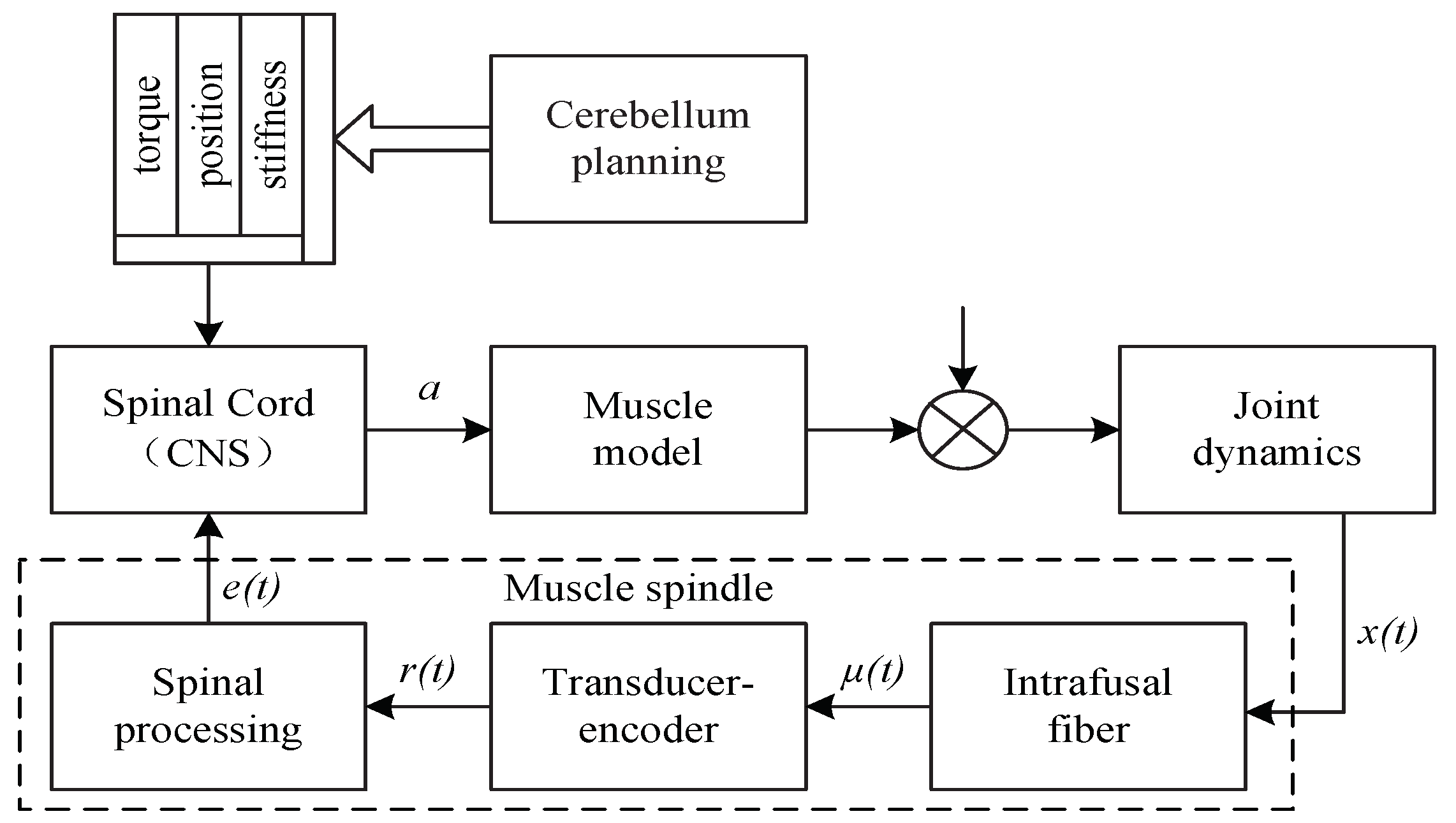
The problem of high-efficient propulsion has been widely studied. However, the efficiency of the robotic fish is still far from the expectations of the application. Why is the propulsive efficiency of the robotic fish much lower than that of the fish in nature? When a fish swims, power is generated by the myotome muscle on either side of the body to overcome the drag [20]. A wave of muscle activation/contraction passes alternately down each side of the body from head to tail in an oscillation cycle. A wave of curvature also travels down the body due to the combined effects of muscle activities, the physical properties of the skeletal elements, and the interaction between the fish’s body and the reactive forces from the water in which it moves [21,22]. The muscles of the fish contract to generate the power for the swimming thrust. In contrast, the motors in the joints of the robotic fish generate the power for the oscillation to achieve forward propulsion. Therefore, applying the control mechanism of the fish muscle onto the motors in the joint space may be a feasible way to improve the efficiency of robotic fish propulsion [23].

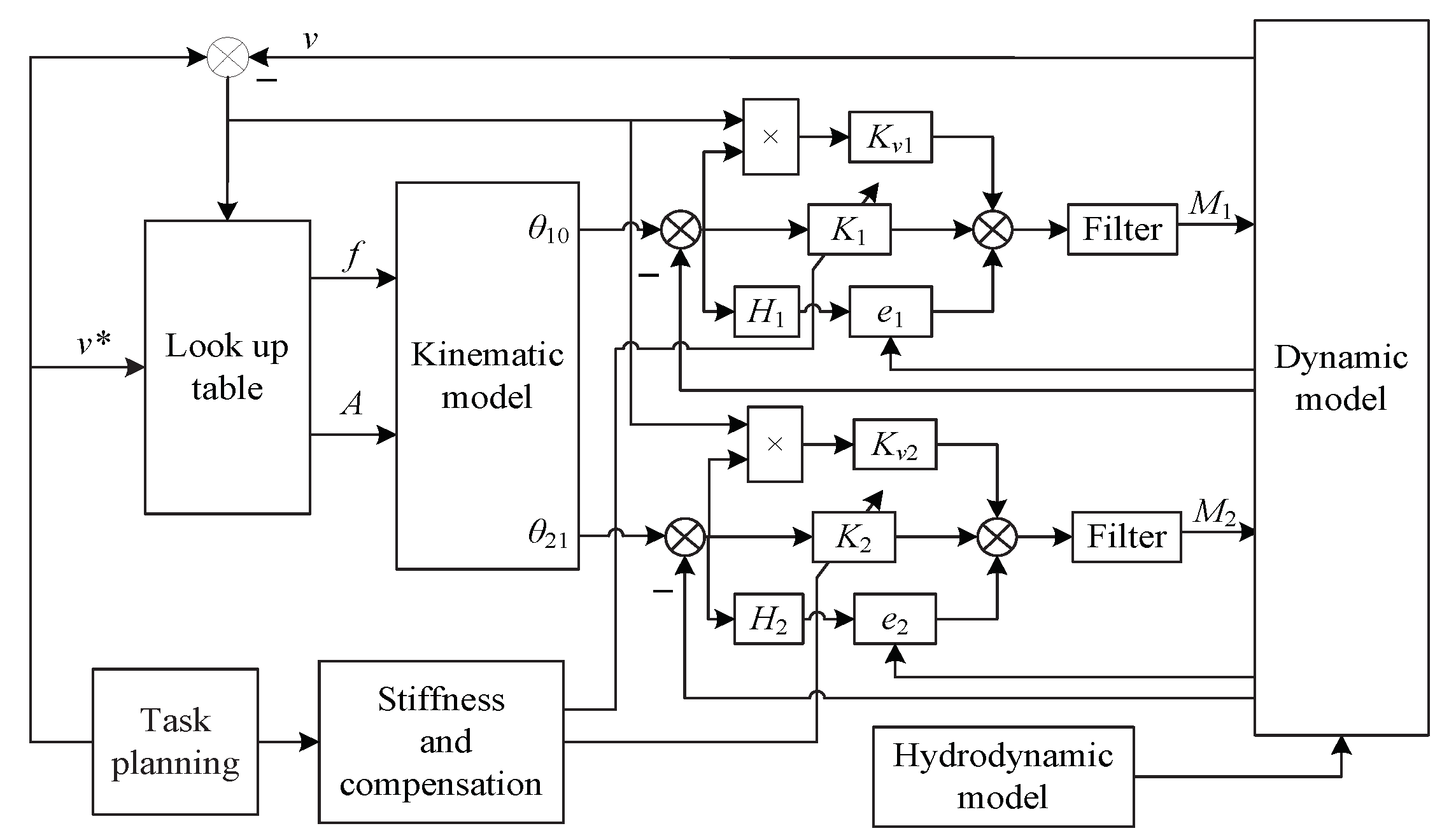
In this paper, we aim to derive the high-efficient methodology from the fish in nature and design a novel closed-loop virtual musculoskeletal control method based on the dynamic model of the robotic fish and the musculoskeletal model of the biotic system. The main contributions of this paper are as follows: (1) a virtual musculoskeletal control method is the first used to raise the propulsion efficiency of robotic fish; (2) a closed-loop control framework, which improves the propulsive efficiency, is constructed by implementing the virtual musculoskeletal mechanism on the dynamic model of the robotic fish; and (3) a series of experiments is conducted to validate the proposed method in various swimming velocities and different parameters of the algorithm and hydrodynamic environment.

The rest of the paper is organized as follows. The mathematical model of a two-joint robotic fish and the problem formulation is stated in Section 2. The model of the musculoskeletal system, the control structure, and the designed strategy are presented in Section 3. Experimental results are presented in Section 4, and the paper ends with the conclusion in Section 5.

2. Modeling of Two-Joint Robotic Fish

2.1. The Kinematic Model

Figure 1a,b shows the prototype of a two-joint robotic fish, which consists of three parts: the head, body, and tail. The length of the robotic fish is $0.6 \mathrm{m}$ and the front $1/3$ part is the head, whose length $L_{\mathrm{h}}$ is $0.2 \mathrm{m}$. $L_1$ and $L_2$ are the length of the body and the tail, respectively. They are greater than that of the driving motor. Let $L_{\mathrm{motor}}$ be $0.1 \mathrm{m}$, $min\left(L_1,L_2\right)>L_{\mathrm{motor}}$. In Figure 1c, $O_1$ is the gravity center of the body and $O_2$ is the gravity center of the tail. $F_0$ is the resistance force of the flow to the fish. $F_1$ is the hydrodynamic force to the body and $F_2$ is the hydrodynamic force to the tail. $D_1$ is the point of the action of $F_1$ while $D_2$ is the point of the action of $F_2$. The solid straight line stands for the midline of robotic fish, while the dashed curve represents the midline of the fish modeled by Lighthill [24]. The $f\left(x\right)$ is the position of the robotic fish to the axis and $g\left(x\right)$ is the position of the live fish to the axis.

$$g(x,t)=(c_{1}x+c_2{x}^2)\sin (\frac{2\pi }{\lambda }x+\omega t)$$

(1)

where $c_1$ and $c_2$ stand for the first and the second coefficient of wave amplitude envelope, respectively; $\lambda$ denotes the wavelength of the body; x is the body axis; and $\omega$ is the body wave frequency.

Moreover, $S_y$ is the area between $f\left(x\right)$ and $g\left(x\right)$. We set $L_1=0.24 \mathrm{m}$ and $L_2=0.16 \mathrm{m}$. Then, $S_y$ obtains its minimum, which indicates that the swing curve of the robotic fish is close to the fish in nature to most. Thus, the motion functions of the two joints are as follows:

$$\left\{\begin{array}{c}{\theta }_{10}\left(t\right)={\theta }_{10A}\times sin\left(2\pi ft\right)\hfill \\ {\theta }_{21}\left(t\right)={\theta }_{21A}\times sin(2\pi ft+\varphi )\hfill \end{array}\right.$$

(2)

where ${\theta }_{10}\left(t\right)$ is the angle between the body and x-axis; ${\theta }_{10A}$ is the amplitude of ${\theta }_{10}\left(t\right)$; ${\theta }_{21}\left(t\right)$ is the angle between the tail and the body, while ${\theta }_{21A}$ is the amplitude of ${\theta }_{21}\left(t\right)$; and $\varphi$ is the phase difference between the two joints.

2.2. The Dynamical Model

The dynamical model of the two-joint robotic fish is established with Lagrange–Euler method shown as follows:

$${\tau }_i=\frac{d}{dt}[\frac{\partial L}{\partial \dot{q_i}}]-\frac{\partial L}{\partial q_i}$$

(3)

where $q_i$ is the system variable, $\dot{q_i}$ is the first derivative of the system variable, ${\tau }_i$ is the generalized force or torque of the system, and i is the number of system variables. As we set that the robotic fish only swims horizontally, the gravitational potential energy is constant. Thus, L is the kinetic energy of the system, which is given in the Appendix A.

$q_i$ represents the three degrees of freedom in the model: ${\theta }_{10}$, the angle of the first joint; ${\theta }_{21}$, the angle of the second joint; and $X_0$, the x-coordinate of the head.

The ${\tau }_i$ is expressed as

$$\begin{array}{c}\hfill \left\{\begin{array}{cc}{\tau }_1\hfill & =\left(\begin{array}{c}{L}_{d1}sin{\theta }_{10}\\ L_{d1}cos{\theta }_{10}\end{array}\right)\times F_1+\left(\begin{array}{c}{L}_{1}sin{\theta }_{10}+L_{d2}sin({\theta }_{21}+{\theta }_{10})\\ L_{1}cos{\theta }_{10}+L_{d2}cos({\theta }_{21}+{\theta }_{10})\end{array}\right)\times F_2+M_1\hfill \\ {\tau }_2\hfill & =\left(\begin{array}{c}{L}_{d2}sin({\theta }_{21}+{\theta }_{10})\\ L_{d2}cos({\theta }_{21}+{\theta }_{10})\end{array}\right)\times F_2+M_2\hfill \\ {\tau }_3\hfill & =F_0·\left(\begin{array}{c}1\\ 0\end{array}\right)+F_1·\left(\begin{array}{c}1\\ 0\end{array}\right)+F_2·\left(\begin{array}{c}1\\ 0\end{array}\right)\hfill \end{array}\right.\end{array},$$

(4)

where ${\tau }_1$, ${\tau }_2$, and ${\tau }_3$ are the non-conservative forces to generalized coordinates ${\theta }_{10}$, ${\theta }_{21}$, and $X_0$, respectively. $M_1$ and $M_2$ are the torques generated by the first and second joint. $F_0$, $F_1$, and $F_2$ are the hydrodynamic forces on the head, body, and tail, respectively.

Neglecting the force of friction, the resistance force to the head is

$$F_0=\frac{1}{2}\rho C_0{V}_0^2{A}_0·{(1,0)}^T,$$

(5)

where $\rho$ is the density of the fluid, $C_0$ is the resistance coefficient of the head, $V_0$ is the velocity of the robotic fish, and $A_0$ is the maximum cross-sectional area of the head.

By simplifying the body as a plane, the hydrodynamic force to the body is

$$F_1=\frac{1}{2}\rho C_1{(V_{c1}·n_1)}^2{A}_1·n_1,$$

(6)

where $C_1$ is the resistance coefficient of the body and $A_1$ is the area of the body. The velocity of the body on point $O_1$ is $V_{c1}={({\dot{X}}_0-L_{1}sin{\theta }_{10}{\dot{\theta }}_{10},L_{1}cos{\theta }_{10}{\dot{\theta }}_{10})}^T$. The normal vector of the body is $n_1={(sin{\theta }_{10},-cos{\theta }_{10})}^T$.

The hydrodynamic force of the tail is predigested in the same way.

$$F_2=\frac{1}{2}\rho C_2{(V_{c2}·n_2)}^2{A}_2·n_2$$

(7)

where $C_2$ is the resistance coefficient of the tail. $A_2$ is the area of the tail. The velocity of the tail on point $O_2$ is $V_{c2}={({\dot{X}}_0-L_{1}sin{\theta }_{10}{\dot{\theta }}_{10}-L_{c2}sin{\theta }_{20}{\dot{\theta }}_{20},L_{1}cos{\theta }_{10}{\dot{\theta }}_{10}+L_{c2}cos{\theta }_{20}{\dot{\theta }}_{20})}^T$, the normal vector of the tail is $n_2={(sin{\theta }_{20},-cos{\theta }_{20})}^T$.

Substitute ${\tau }_i$ and L into Equation (3). The dynamic model of the robotic fish is

$$D\left(Q\right)\ddot{Q}+H(Q,\dot{Q})+G\left(Q\right)=\tau$$

(8)

where $D\left(Q\right)$ is the inertia matrix, Q is the joint variable, $H(Q,\dot{Q})$ is the vector of centrifugal force and the Coriolis force, and $G\left(Q\right)$ is the gravity vector. Their details are given in the Appendix A.

2.3. The Propulsive Efficiency

The propulsive efficiency is defined as the ratio of the useful work to push the fish forward and the total work consumed by all components of the robotic fish.

$$\eta =\frac{W_{useful}}{W_{total}}$$

(9)

In our model, the components that need to be actuated are the two joints. The total work in one period is

$$W_{total}={\int }_0^T(M_1\left(t\right){\dot{\theta }}_{10}\left(t\right)+M_2\left(t\right){\dot{\theta }}_{21}\left(t\right))dt.$$

(10)

As the swing of the joints generates the hydrodynamic force to push the fish forward in the X direction, the useful work in one period is

$$W_{useful}={\int }_0^T(F_{1x}\left(t\right)+F_{2x}\left(t\right))·V_0\left(t\right)dt.$$

(11)

3. The Virtual Musculoskeletal Methodology

3.1. Modeling the Muscular Skeletal System

The mathematic model of the musculoskeletal system of the fish, shown in Figure 2, includes three parts: The muscles are actuators to produce torque. The spindles in the extrafusal muscles are mechanoreceptors to provide dynamic feedback for the closed-loop control. The central nervous system (CNS) in the spinal cord operates the dynamic motions of these muscles. The movement is driven by agonist muscles and antagonist muscles controlled by the CNS’s excitation signals. The excitation signals are produced from two sources of information: (1) the cerebellum plans the control goal in joint space according to the movement task and (2) the CNS unifies this goal and the feedback signals from the spindles to send signals to the muscles. The CNS adjusts the position and speed of the swing and varies the total stiffness and viscosity over a considerable range. This adjustment realizes the compliant action to the water environment.

3.1.1. The Model of the Muscle

The three-element Hill muscle model is a representation of the muscle mechanical response. The model is constituted by a contractile element (CE) and two nonlinear spring elements: one in series (SE) and another in parallel (PE). Due to the series connection of the tendon and the muscle belly, by ignoring the angle between them, the force of the muscle is equal to the force produced by the parallel units consisting of CE and PE.

The force–length relation of PE is

$$\frac{F^{\mathrm{PE}}}{F_{max}}=K^{\mathrm{PE}}=\left\{\begin{array}{cc}0\hfill & \mathrm{if}{L}^{\mathrm{PE}}<L_{\mathrm{slack}}^{\mathrm{PE}}\hfill \\ k^{\mathrm{PE}}\left[{(\frac{L^{\mathrm{PE}}}{L_{\mathrm{slack}}^{\mathrm{PE}}})}^2-1\right]\hfill & \mathrm{if}{L}^{\mathrm{PE}}\ge L_{\mathrm{slack}}^{\mathrm{PE}}\hfill \end{array}\right.,$$

(12)

where $F^{\mathrm{PE}}$ is the force generated by PE, $L^{\mathrm{PE}}$ is the current length of PE while $L_{\mathrm{slack}}^{\mathrm{PE}}$ is the length when muscle is slack, $k^{\mathrm{PE}}$ is a coefficient relating to the property of muscle fibers, and $K^{\mathrm{PE}}$ is the coefficient to describe the rate to the maximum force.

The force–length equation and the force–speed equation illustrate the feature of CE. In Equations (13) and (14), the force is a quadratic function to the length and a hyperbolic function to the speed.

$$\frac{F_L^{CE}}{F_{max}}=K_L^{CE}=1-{\left(\frac{L^{CE}-L_0^{CE}}{w}\right)}^2$$

(13)

$$\frac{F_v^{CE}}{F_{max}}=K_v^{CE}=\frac{F_{max}{v}_{max}\beta -\alpha v}{F_{max}(\beta v_{max}+v)}$$

(14)

where $L^{\mathrm{CE}}$ is the muscle length, $L_0^{\mathrm{CE}}$ is the length when the muscle achieves maximum isometric contraction force $F_{\max }$, w is used to control the width of the curve, $K_L^{\mathrm{CE}}$ is the force–length coefficient of contraction element, $v_{max}$ is the maximum speed of muscle contraction, $\alpha$ and $\beta$ are coefficients relating to characteristics of muscle fibers, and $K_v^{\mathrm{CE}}$ is the force–speed coefficient.

3.1.2. The Model of the Spindle

The spindle produces the feedback information with three component processes illustrated in Figure 2. At first, the intrafusal fibers transfer the movement of muscle to nerve stretch. The fibers mechanically filter muscle length $x\left(t\right)$ to a stretch of the sensory ending $\mu \left(t\right)$. This component is given by a nonlinear differential equation:

$$\frac{d\mu \left(t\right)}{dt}+b(\frac{c\mu \left(t\right)-x\left(t\right)+g}{x\left(t\right)-\mu \left(t\right)-g})=\frac{dx\left(t\right)}{dt},$$

(15)

where b and c are constants that affect the degree of nonlinearity, and g is a reference length specifying the lower bound of the position range where the muscle spindle responds to stimuli.

Then, the transducer encoder converts the nerve stretch into neural signal $r\left(t\right)$. The linear dynamics of the transducer encoder is

$$r\left(t\right)=N(\mu \left(t\right)+{\tau }_{ed}\frac{d\mu \left(t\right)}{dt}),$$

(16)

where N represents the small-signal sensitivity of the receptor and ${\tau }_{\mathrm{ed}}=0.1$ s is the time constant of encoder dynamics.

Finally, $r\left(t\right)$ is conducted to the spinal cord to process an electromyographic (EMG) signal $e\left(t\right)$ for muscle activation. The reflex pathway through the spinal cord is modeled as a time delay of $0.03$ s.

$$e\left(t\right)=r(t-0.03)$$

(17)

3.1.3. The Excitation Model of the CNS

The CNS mediates the task command and the reflex from the muscle and then yields signals to activate the muscles. It incentives the contraction of muscle by EMG that comprises the information from the cerebellum and the feedback from the spindle. The information in the EMG is separated into two parts: One is from the cerebellum. Its strength is represented by a coefficient $a(0<a<1)$. The other is from the spindle. The $e\left(t\right)$ represents the excitation signals related to the spindle information. Thus, adding the EMG into the muscle model in Equations (12)–(14), the equation of the muscle excited by CNS is

$$F=(K_L^{CE}{K}_v^{CE}(a+e\left(t\right))+K^{PE})F_{max}.$$

(18)

3.2. Virtual Musculoskeletal Method

Abstracting the strategy from the bionic model, we design the virtual musculoskeletal methodology for the activation of the joints.

Equation (18) contains the mechanics of the muscle and the activation of CNS. Suppose that the agonist and antagonist muscles have the same stiffness, maximum force, and spindle signal, then the torques generated by both muscles at the joint are

$$M_{ag}=(K_L^{CE}{K}_v^{CE}(a+e\left(t\right))+K^{PE})M_{max},$$

(19)

$$M_{an}=-(K_L^{CE}{K}_v^{CE}(a+e\left(t\right))+K^{PE})M_{max},$$

(20)

where $M_{max}$ is the maximum torque of each muscle.

Equation (19) subtracts Equation (20), and therefore the torque of the muscular joint is

$$M=(2K_L^{CE}{K}_v^{CE}a+2K_L^{CE}{K}_v^{CE}e\left(t\right)+2K^{PE})M_{max},$$

(21)

In Equation (21), $K_L^{CE}$ and $K^{PE}$ indicate the relationship between the length of the muscle and the torque, and $M_{max}$ is a constant. We set $K\mathsf{\Delta }\theta$ to take the place of $2K_L^{CE}{M}_{max}$ and $2K^{PE}{M}_{max}$. Thus, the torque of the joint is

$$M=(K{K}_v^{CE}a+K{K}_v^{CE}e\left(t\right)+K)\mathsf{\Delta }\theta ,$$

(22)

where $\mathsf{\Delta }\theta$ represents the position of the muscle to the equilibrium.

The torque of the joint includes three parts; parameter K is the stiffness of the joint and $K{K}_v^{\mathrm{CE}}a$ represents the response of the muscle to the control signal from CNS. As our goal is to control the robotic fish to follow a given speed, this part could be replaced by adjusting the speed. The feedback from the spindle $e\left(t\right)$ contains the nonlinearity, $K{K}_v^{\mathrm{CE}}$ is replaced by a coefficient H to adjust the feedback intensity of the spindle. Therefore, the equation of the torque of the joint is simplified as

$$M=(K_v(v^{*}-v)+He\left(t\right)+K)\mathsf{\Delta }\theta ,$$

(23)

where $v^{*}$ is the planned swimming speed of the robotic fish and v is the real swimming speed of the fish.

Equation (23) shows that the torque of the joint contains three parts of activation: (1) the adjustment from the CNS which is dependent on the task planning and the real swimming state, (2) the feedback signal from the muscle spindle, and (3) the stiffness of the joints set by the task planning. To control the robotic fish, $\mathsf{\Delta }\theta$ represents the deviation of a given angle and the real angle. Therefore, the virtual musculoskeletal control method is

$$M=\left[K_v(v^{*}-v)+He(\theta ,\dot{\theta })+K\right]({\theta }^{*}-\theta ),$$

(24)

where $e(\theta ,\dot{\theta })$ indicates the spindle-like feedback in the controller and H is the coefficient of this feedback. The spindle-like feedback is designed as a fuzzy controller, whose inputs are the angle and the angular velocity. This controller imitates the nonlinearity of the muscle feedback well [23]. This controller needs three kinds of information from the planning algorithm: a given swimming speed, a set stiffness, and a given angle of the joint.

As the signals delay in the spinal cord and nerve system, a low-pass filter in Equation (25) is added after the given signal to the joint.

$$d\left(s\right)=\frac{1}{{\tau }_{ed}s+1}$$

(25)

3.3. The Closed-Loop Control Structure

The control algorithm is designed to control the robotic fish compliantly and efficiently. When swimming, the biological fish changes the feature of muscles to control the body’s posture and the swing speed to fit the water environment. In the control process, the fish perceives the flow field of the water. Then, the nervous system mixes this information with the posture and the swimming speed to decide how to adjust its swimming parameters. When the neural signals reach the muscles, the muscles contract for the swing of the fish. Consequently, the fish efficiently swims at an expected speed. In this way, the control process designed to mimic the fish in nature is shown in Figure 3.

The robotic fish is controlled in a closed-loop procedure. At first, the task planning module sets the swimming velocity and the stiffness of both joints. The lookup table is a fitting curve function, shown in Figure 4, which outputs the frequency f and the amplitude A of the wave of the robotic fish (All subsequent curve figures in the paper are drawn using MATLAB software.). We regulate the input of this table according to the error between the set velocity and the actual swimming velocity. This negative feedback helps the robotic fish follow the set velocity from the task planning. Second, Equation (2) transforms the wave to angles in the joint space. Third, Equation (24) is decomposed into two equations of two joints.

$$\left\{\begin{array}{c}{M}_1=d\left(s\right)[K_{v1}(v^{*}-v)+H_1{e}_1({\theta }_{10},\dot{{\theta }_{10}})+K_1]({\theta }_{10}^{*}-{\theta }_{10})\hfill \\ M_2=d\left(s\right)[K_{v2}(v^{*}-v)+H_2{e}_2({\theta }_{21},\dot{{\theta }_{21}})+K_2]({\theta }_{21}^{*}-{\theta }_{21})\hfill \end{array}\right.$$

(26)

where $M_1$ and $M_2$ are the torques to drive the joints, $K_{v1}$ and $K_{v2}$ are the gains for the velocity deviation, $H_1$ and $H_2$ are the intensive coefficients of the feedback in the joints, $e_1$ and $e_2$ are the virtual spindle functions, $K_1$ and $K_2$ are the stiffness set by the task planning module, and “*” indicates that the value is the given value.

The last part of the procedure is the movement of the robotic fish under the excitation of $M_1$ and $M_2$. Two models restrain the robotic fish: one is the dynamic model, which is analyzed by the Lagrange method, the other is the hydrodynamic model, which describes how the flow generates the force on the parts of the robotic fish. While the fish is swimming, the swimming velocity and the angles of the joints are fed back to the control algorithm in real-time.

4. Performance Evaluation

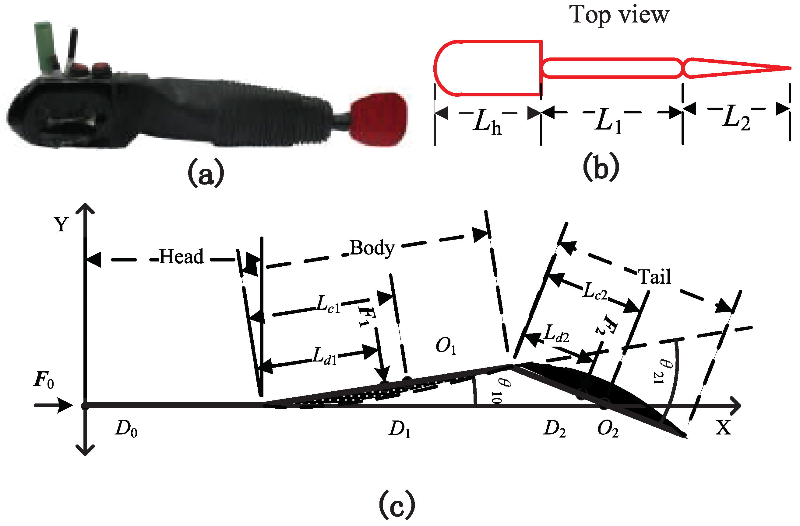
The wavelength of the body is $\lambda =0.75 \mathrm{m}$. Therefore, the phase difference is $1.57 \mathrm{rad}$. To ensure the endpoints of the body and the tail coincide with the corresponding points on the midline of the live fish, let ${\theta }_{10A}=0.3144 \mathrm{rad}$ and ${\theta }_{21A}=1.0123 \mathrm{rad}$. The parameters in Figure 1 are shown in

Table 1. The specific values of the parameters in Figure 1.

Parameters	${\mathit{A}}_0$	${\mathit{A}}_1$	${\mathit{A}}_2$	${\mathit{L}}_{\mathit{c}1}$	${\mathit{L}}_{\mathit{d}1}$	${\mathit{L}}_{\mathit{c}2}$	${\mathit{L}}_{\mathit{d}2}$	${\mathit{m}}_0$	${\mathit{m}}_1$	${\mathit{m}}_2$
Value	$0.03 {\mathrm{m}}^2$	$0.05 {\mathrm{m}}^2$	$0.05 {\mathrm{m}}^2$	$0.12 \mathrm{m}$	$0.12 \mathrm{m}$	$0.12 \mathrm{m}$	$0.12 \mathrm{m}$	$0.8 \mathrm{kg}$	$0.4 \mathrm{kg}$	$0.5 \mathrm{kg}$

. The hydrodynamic parameters and controller parameters are shown in

Table 2. The specific values of the hydrodynamic and controller parameters.

Parameters	${\mathit{C}}_0$	${\mathit{C}}_1$	${\mathit{C}}_2$	$\mathit{\rho }$	${\mathit{K}}_1$	${\mathit{K}}_2$	${\mathit{H}}_1$	${\mathit{H}}_2$	${\mathit{K}}_{\mathit{v}1}$	${\mathit{k}}_{\mathit{v}2}$
Value	$0.9$	$1.54$	$1.54$	$1000 \mathrm{kg}/{\mathrm{m}}^3$	5	16	1	9	0.1	0.1

.

The virtual musculoskeletal methodology in this paper is compared with the proportion control, which is a widely used method in the joint space of the robotic fish. In the figures of this paper, the subscript “PM” means the proportion method, and “VMM” means the virtual musculoskeletal method.

We evaluate the performance when the robotic fish is controlled via the virtual Musculoskeletal closed-loop algorithm. The simulation results are obtained from three aspects: (1) the robotic fish swims in the steady flow field; (2) the robotic fish swims in the Karman vortex field; (3) how the controller’s parameters affect the efficiency and other indices of performance.

4.1. In Steady Flow

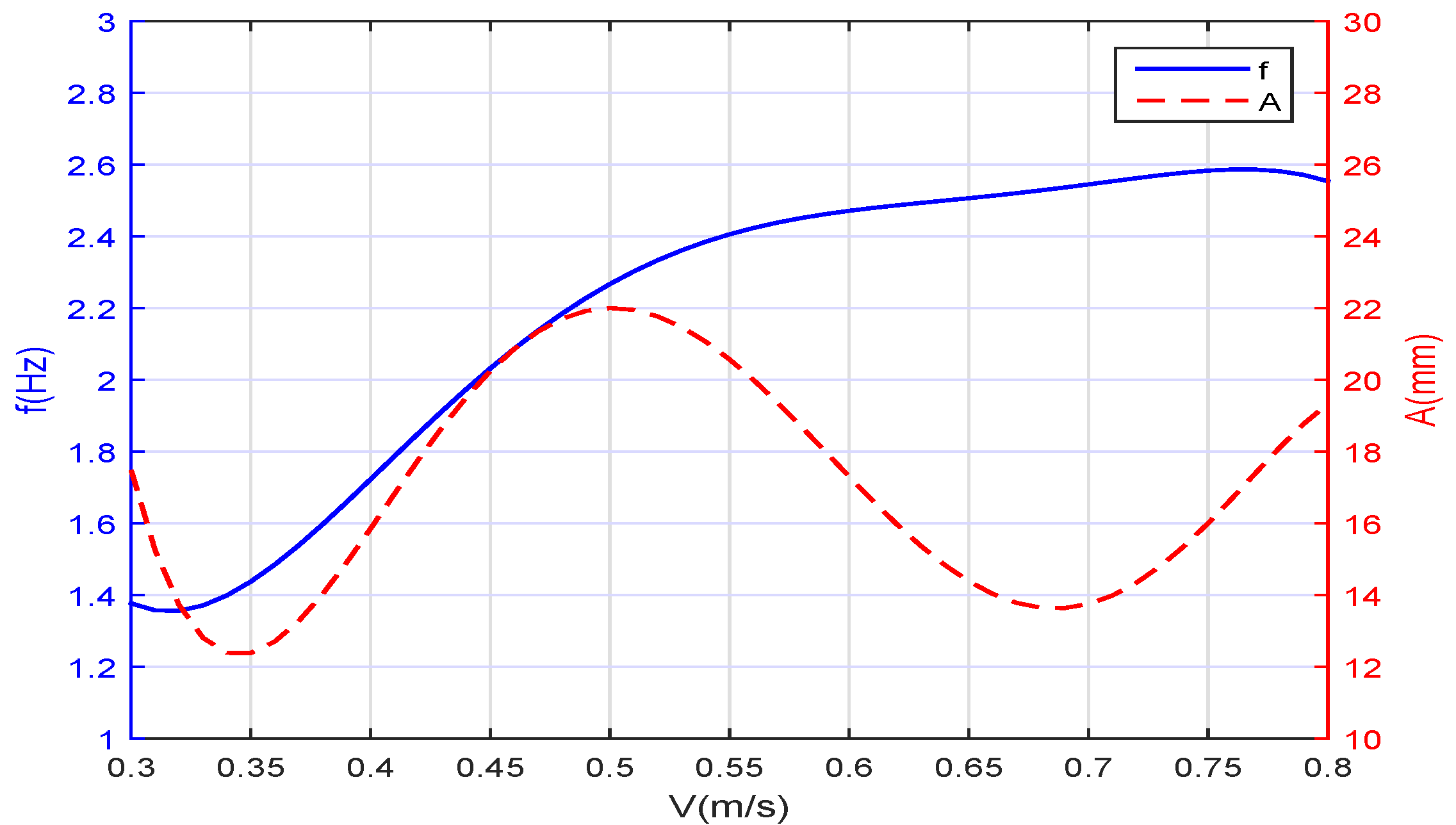
The robotic fish swims in a steady flow. The given speed is $v^{*}=0.4 \mathrm{m}/\mathrm{s}$ at the beginning, and it steps to $0.5 \mathrm{m}/\mathrm{s}$ at $15 \mathrm{s}$. How the feedback of the speed in the control structure stabilizes the swimming speed is illustrated in Figure 5 and Figure 6. In Figure 4, the relationships between the forward speed v and the frequency f and the amplitude A of the oscillation are depicted. 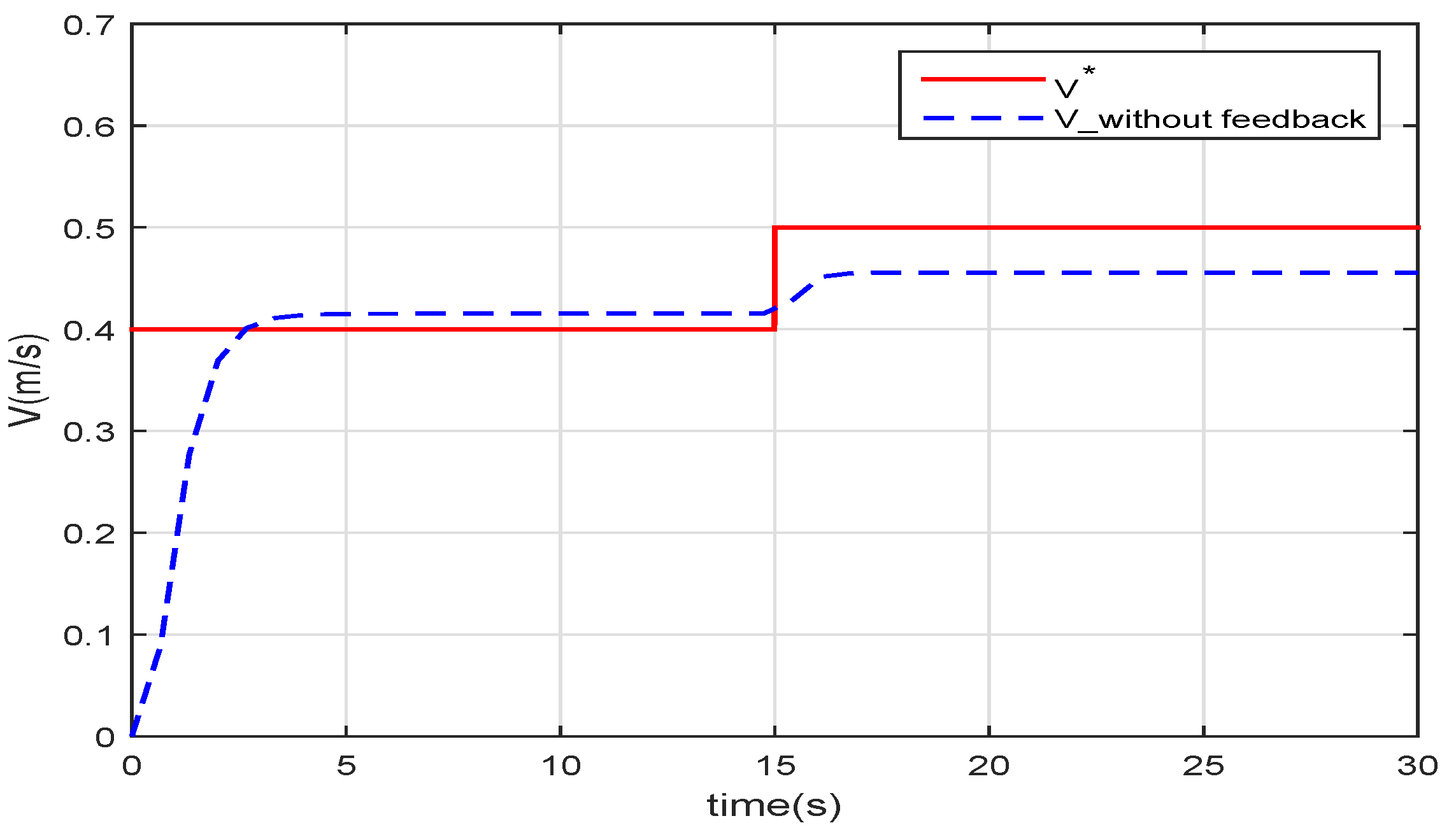When we set the frequency and the amplitude for desired swimming speed, such as $0.4 \mathrm{m}/\mathrm{s}$ and $0.5 \mathrm{m}/\mathrm{s}$, Figure 5 shows that if the speed feedback is not added to form the closed-loop control, there will be a deviation between the real swimming speed $v_{\_\mathrm{without}\mathrm{feedback}}$ and the given speed $v^{*}$.

Because the robotic fish model is not exactly the same as the live fish, the function derived from the data of the fish in nature does not fit the robotic fish perfectly. Additionally, the speed cannot follow the given value if there is a disturbance in the water.

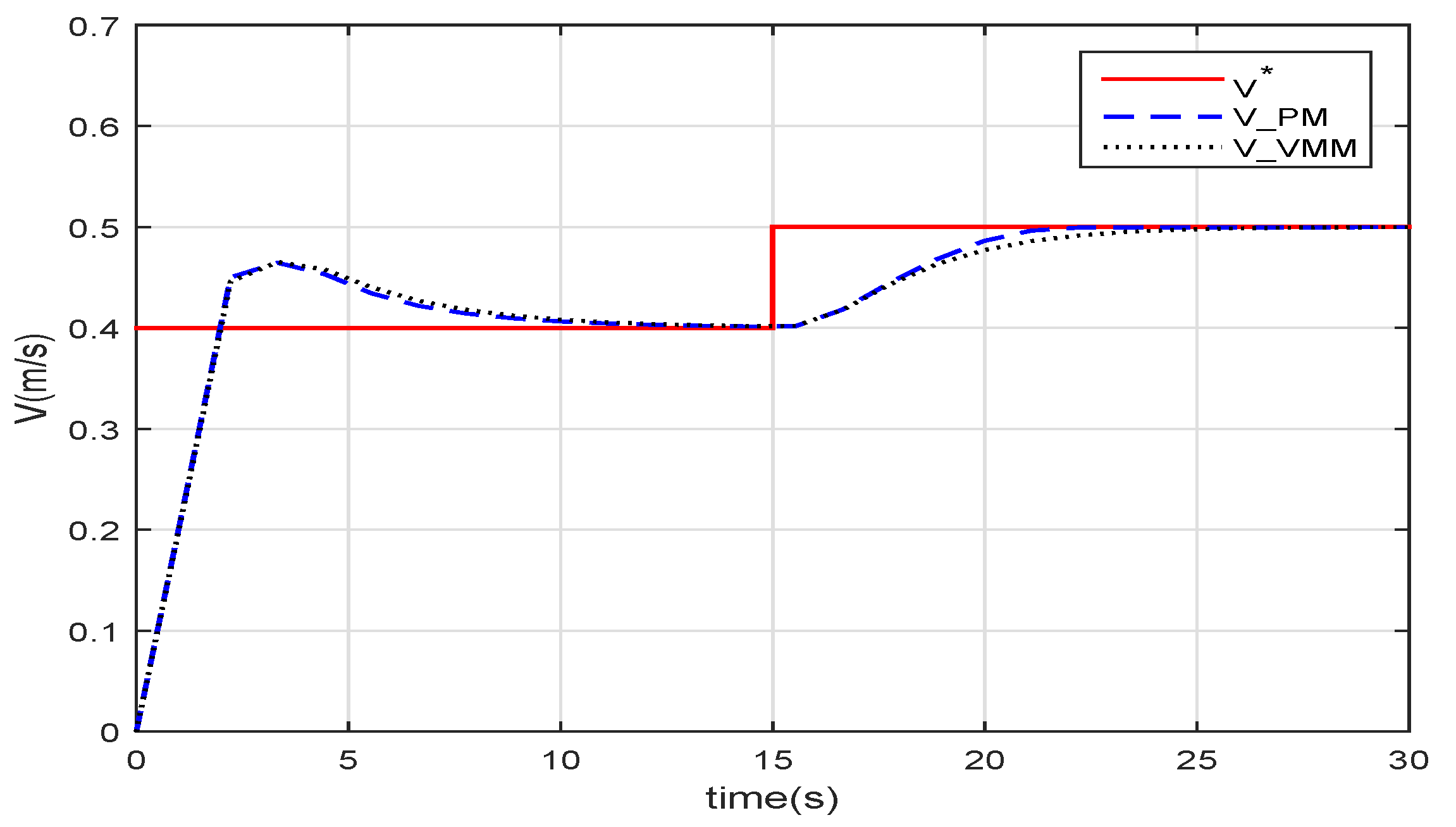
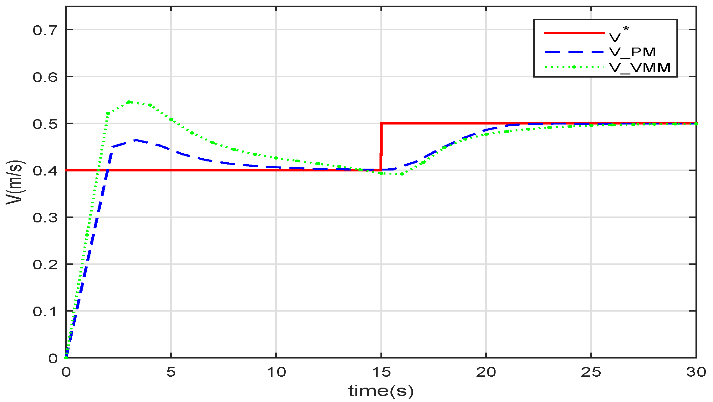
Figure 6 sketches the speed following when the robotic fish is controlled with speed feedback. The speed of the PM($v_{\_\mathrm{PM}}$) and the VMM($v_{\_\mathrm{VMM}}$) both follow the given speed. After the step at $15 \mathrm{s}$, the response time of the VMM and that of the PM is very close.

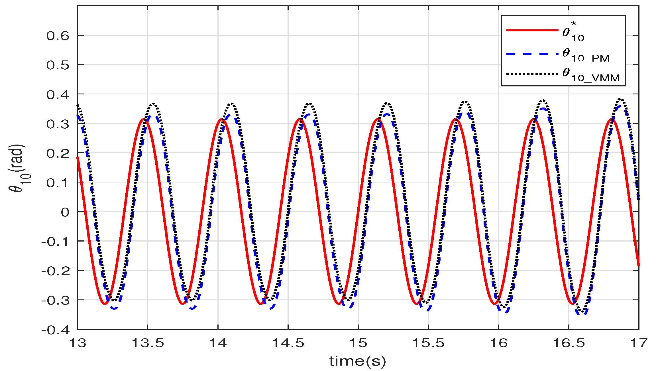
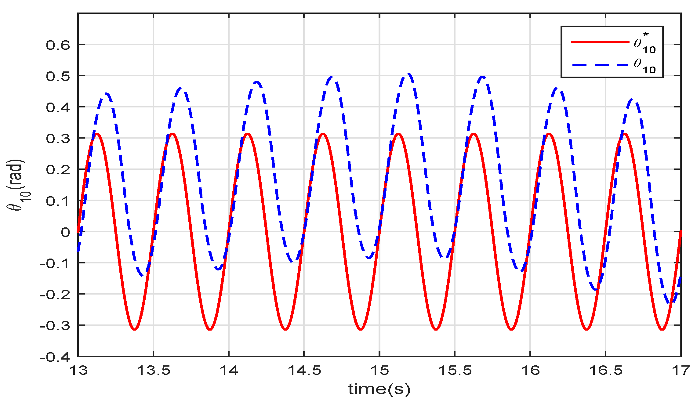
Figure 7 shows the angle of the joint between the head and the body. Both curves of the two control methods are stable sinusoidal waveforms that follow the given ${\theta }_{10}$ with a ${30}^{°}$ delay. This delay is caused by the calculation time, the response time of the dynamic model, and the hydrodynamic model. The curve of VMM has an offset of the amplitude because of the VMM complaints to the force from the water. As the hydrodynamic forces on the robotic fish are not completely symmetrical, the offset of the amplitude is added in the wave.

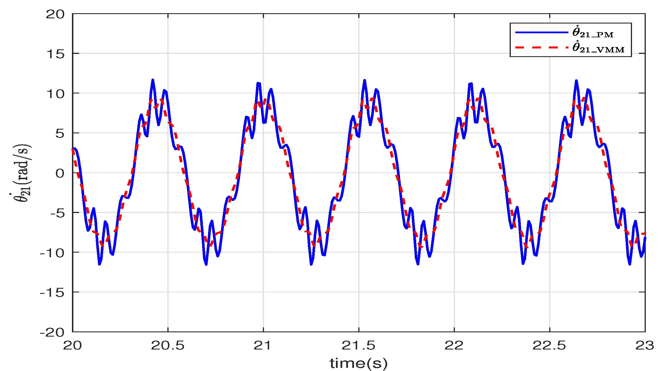
The angular velocity of the tail relative to the head is illustrated in Figure 8. The angular velocity of VMM (${\dot{\theta }}_{21\_\mathrm{VMM}}$) changes more smoothly than that of PM (${\dot{\theta }}_{21\_\mathrm{PM}}$). The virtual spindle model in the VMM adjusts the torque according to the angle and the angular velocity of the joints. This adjustment mimics how the muscles change the stretching speed and power to improve the smoothness of the movements.

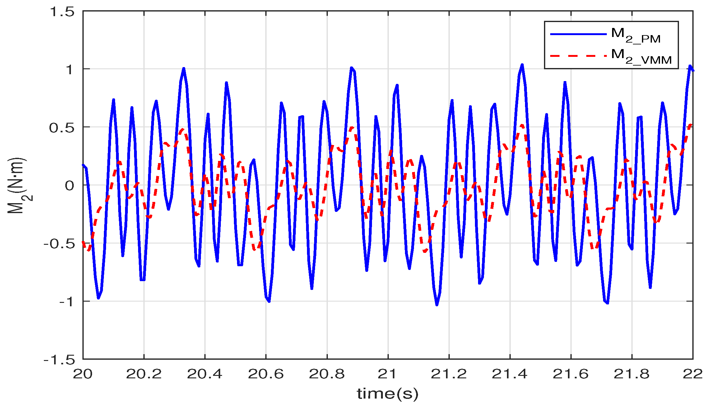
Figure 9 shows the output torque of the motor in the second joint. The magnitude of $M_2$ of the VMM ($M_{2\_\mathrm{VMM}}$) is $0.5 \mathrm{Nm}$ less than that of the PM ($M_{2\_\mathrm{PM}}$); $M_2$ of the VMM also changes more smoothly than the PM. In the closed-loop control, the VMM leads the flexibility and adaptability of the muscles into the controller in the joint space. Thus, the joint can adapt to the environment to avoid the output torque changes radically. Thereby, the smoothness of the torque can reduce energy consumption. Figure 10 depicts the feedback signal of the virtual spindle model in the VMM. The fuzzy controller $e\left(t\right)$ generates the spindle-like feedback signal to regulate the closed-loop controller to fit the disturbances in the environment. $e_1$ and $e_2$ are periodic signals transformed from the angular velocity and the angle of the joints. As the torque and the hydrodynamic force interact with the movements of the joints, $e_1$ and $e_2$ add the same-frequency virtual spindle signals onto the sinusoidal motion of the joints. Therefore, the body and the tail fin can use the hydrodynamic force of the fluid better to reduce energy consumption and improve propulsive efficiency.

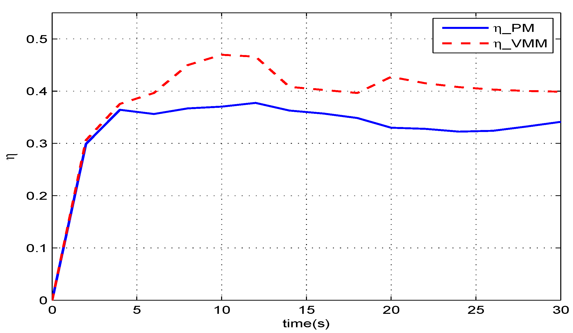
Figure 11 gives the results of how much the VMM increases the propulsive efficiency of the robotic fish. Before $2.5 \mathrm{s}$, in the start-up phase, these two methods have the same efficiency. When the robotic fish reaches the speed of $0.4 \mathrm{m}/\mathrm{s}$, the efficiency of the VMM (${\eta }_{\_\mathrm{VMM}}$) is one percentage point higher than that of the PM (${\eta }_{\_\mathrm{PM}}$). The given speed jumps to $0.5 \mathrm{m}/\mathrm{s}$ at $15 \mathrm{s}$, and both efficiencies decrease with increasing speed. At $0.5 \mathrm{m}/\mathrm{s}$, the VMM plays a more significant role in improving the propulsive efficiency. The efficiency of VMM is $32\%$, which is $3.4$ percentage points higher than that of the PM.

4.2. In Karman Vortex Flow

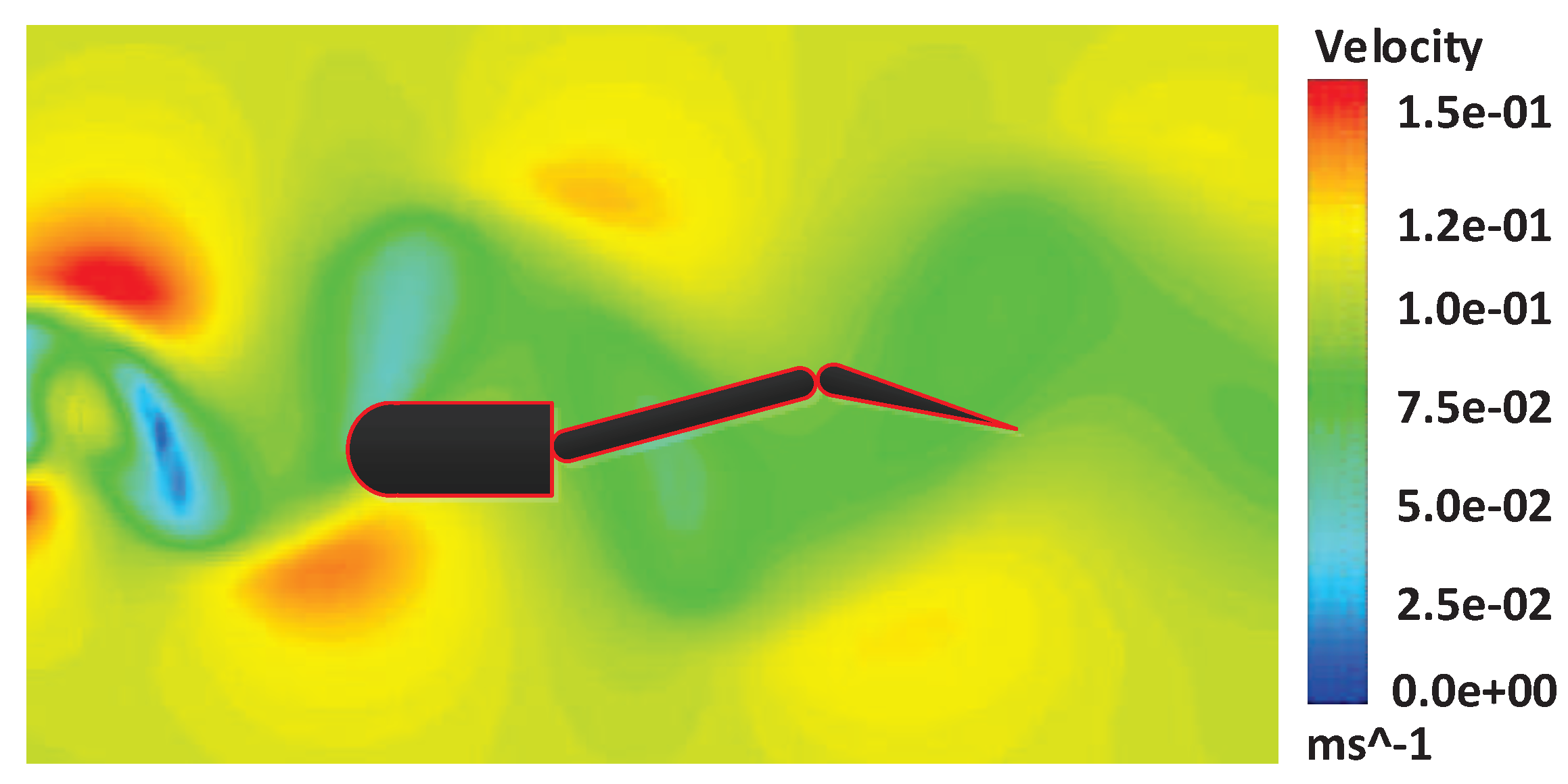
Fish often swim in water that is full of disturbances. Therefore, the control strategy of the robotic fish must adapt to the flow environment. The Karman vortex is a typical vortex flow field for the environment test of the robotic fish. We extend the analysis of the algorithm in a steady flow to the Karman vortex flow field. We generate the Karman vortex shown in Figure 12 in FLUENT and add the vortex to the swimming environment of the robotic fish.

The speed of the robotic fish swimming in the Karman vortex is depicted in Figure 13. The VMM follows the given speed faster at the beginning, whose rise time is $0.4 \mathrm{s}$ shorter than the PM. The overshoot of the VMM, meanwhile, is $18\%$ greater than that of the PM. The VMM, which has the characteristics of muscles, can use the flow vortex to boost the speed. Consequently, the robotic fish loses some ability to adjust its speed, leading to a greater overshoot. At $15 \mathrm{s}$, the overshoot of the VMM still affects the response of the speed that the following of the speed is a little slower compared with the PM.

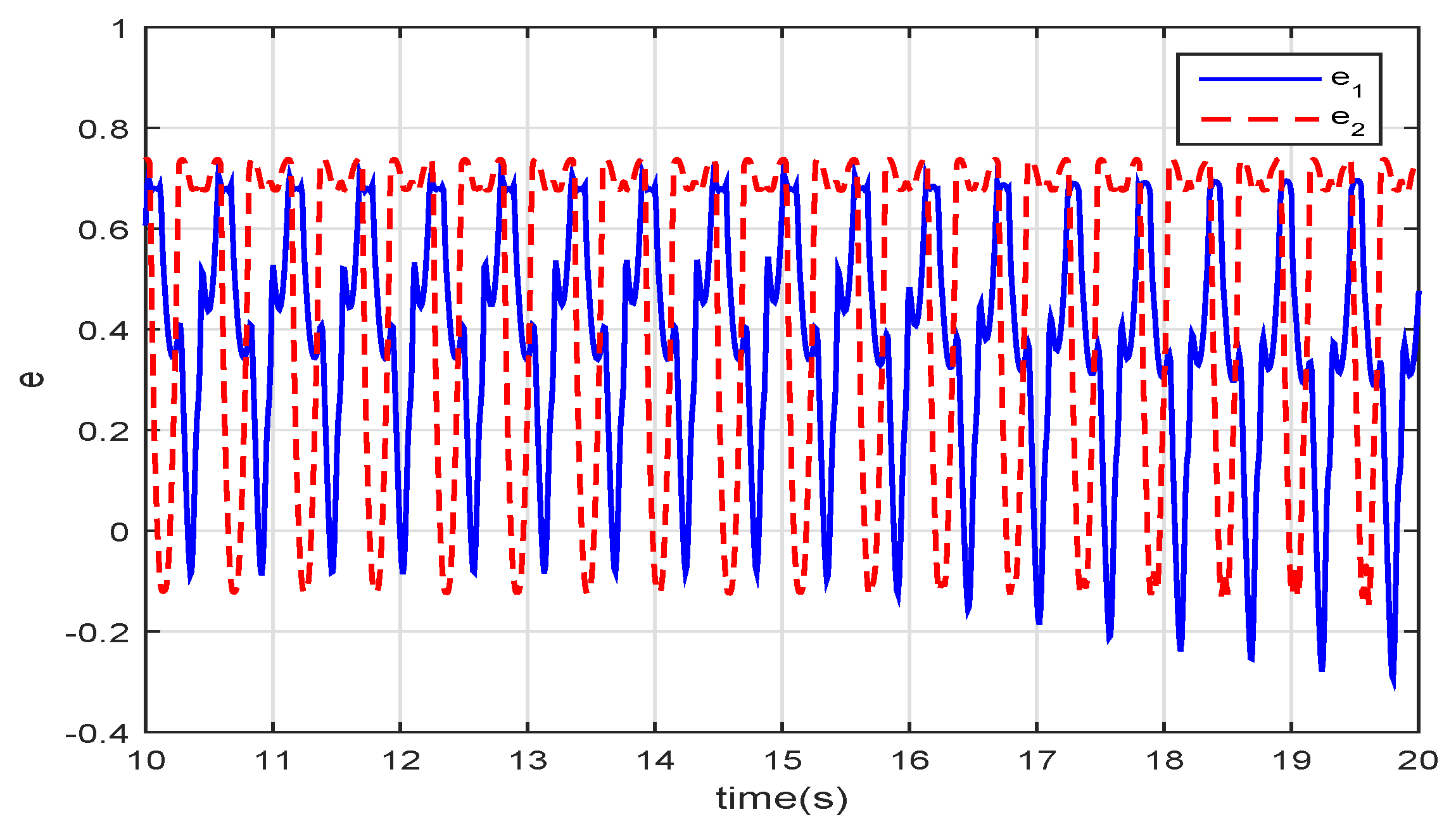
The angles of the joints in Figure 14 show that the VMM adjusts the movements of the robotic fish to adapt to the vortex in the water. As a result, the robotic fish swims with higher efficiency than controlled via the PM. The actual angle of the first joint has phase lag and positive deviation. The phase lag of the waveform is ${38}^{°}$, which is greater than the lag in the steady water; the offset is $1.5 \mathrm{rad}$ because the vortex affects the hydrodynamic force on the robotic fish.

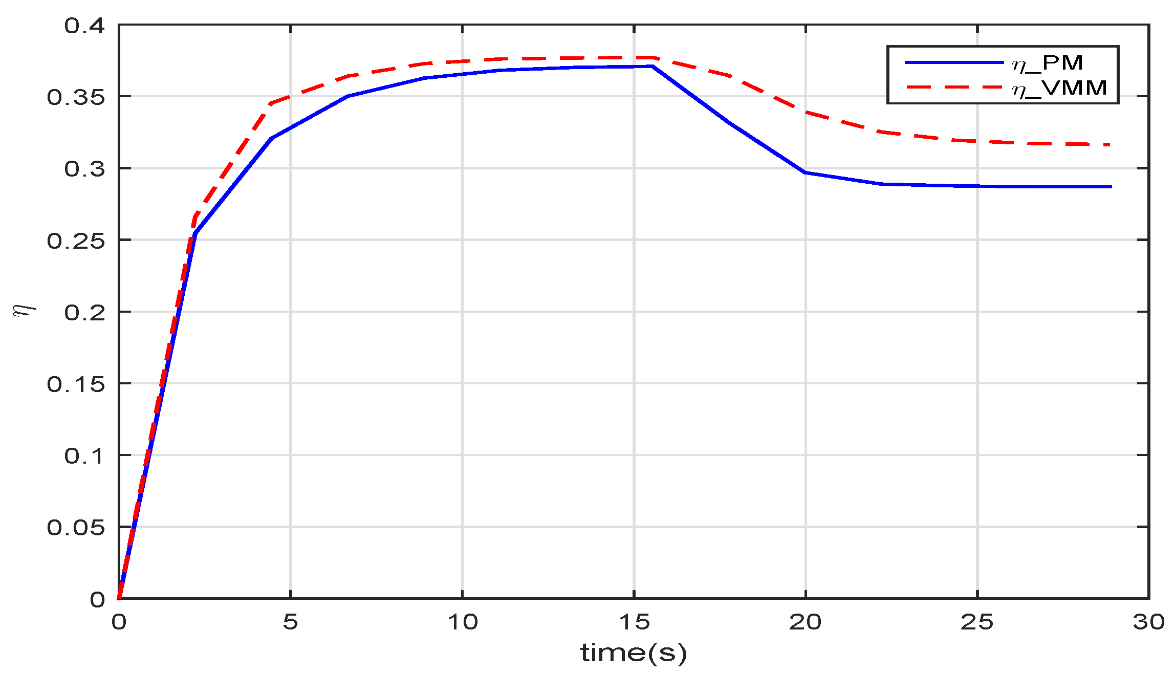
In the Karman vortex, the VMM can improve the propulsive efficiency more significantly than it does in the steady flow. Figure 15 illustrates that the VMM increases the efficiency about $10\%$ than the PM. When the speed is $0.4$ m/s, the $\eta$ of PM is $36\%$ while the $\eta$ of VMM reaches $47\%$. At $0.5$ m/s, the $\eta$ of PM is $33\%$ and the $\eta$ of VMM is $40\%$. The vortex in the water contains the energy to generate the hydrodynamic force on the robotic fish. The virtual muscular method takes the compliance into the joints. The compliant joints can use the energy of vortex street better; thus, the robotic fish consumes less energy to produce motive force for the forward motion.

4.3. The Affection of the Parameters

The closed-loop controller via the VMM includes several parameters, the values of which are significant to the performance of the robotic fish. This subsection analyzes the relations between the parameters and the efficiency to provide references for the parameter setting. The experiment fixes other parameters and changes each parameter to test how it affects efficiency.

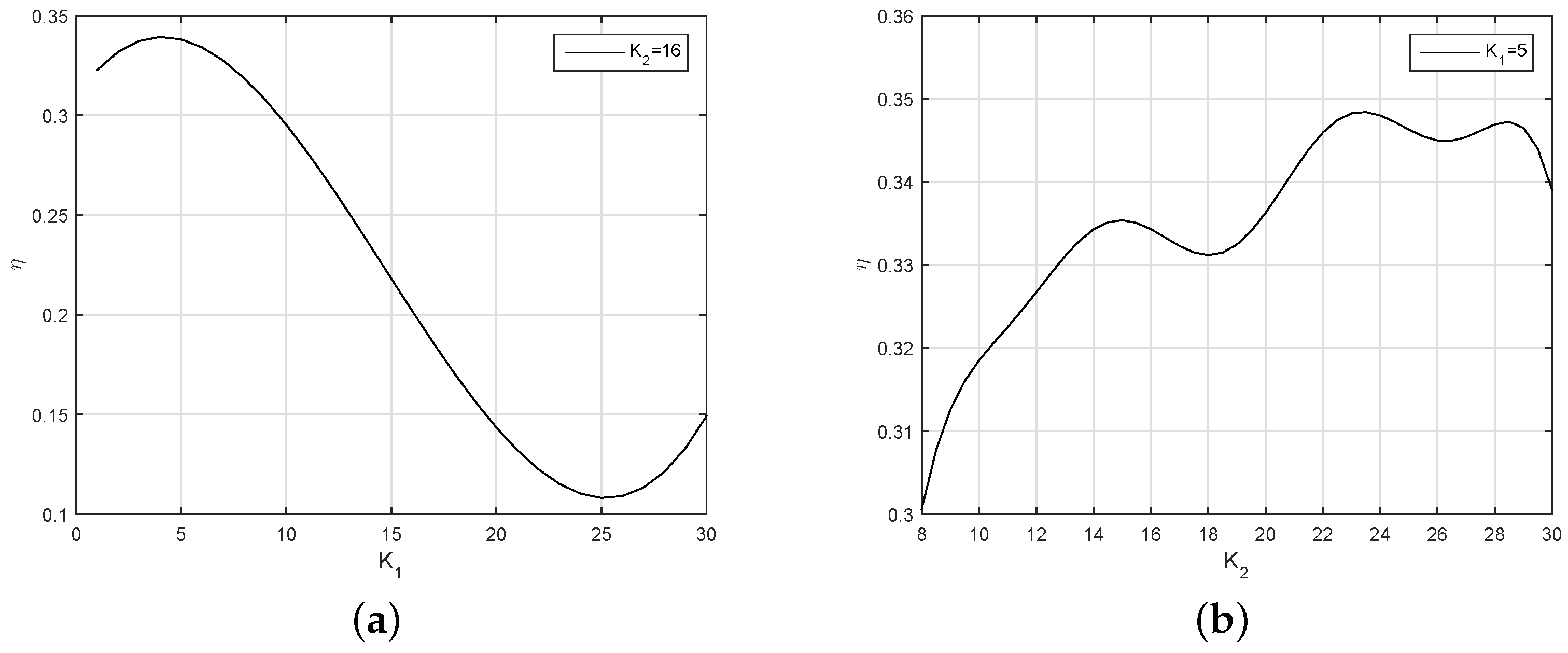
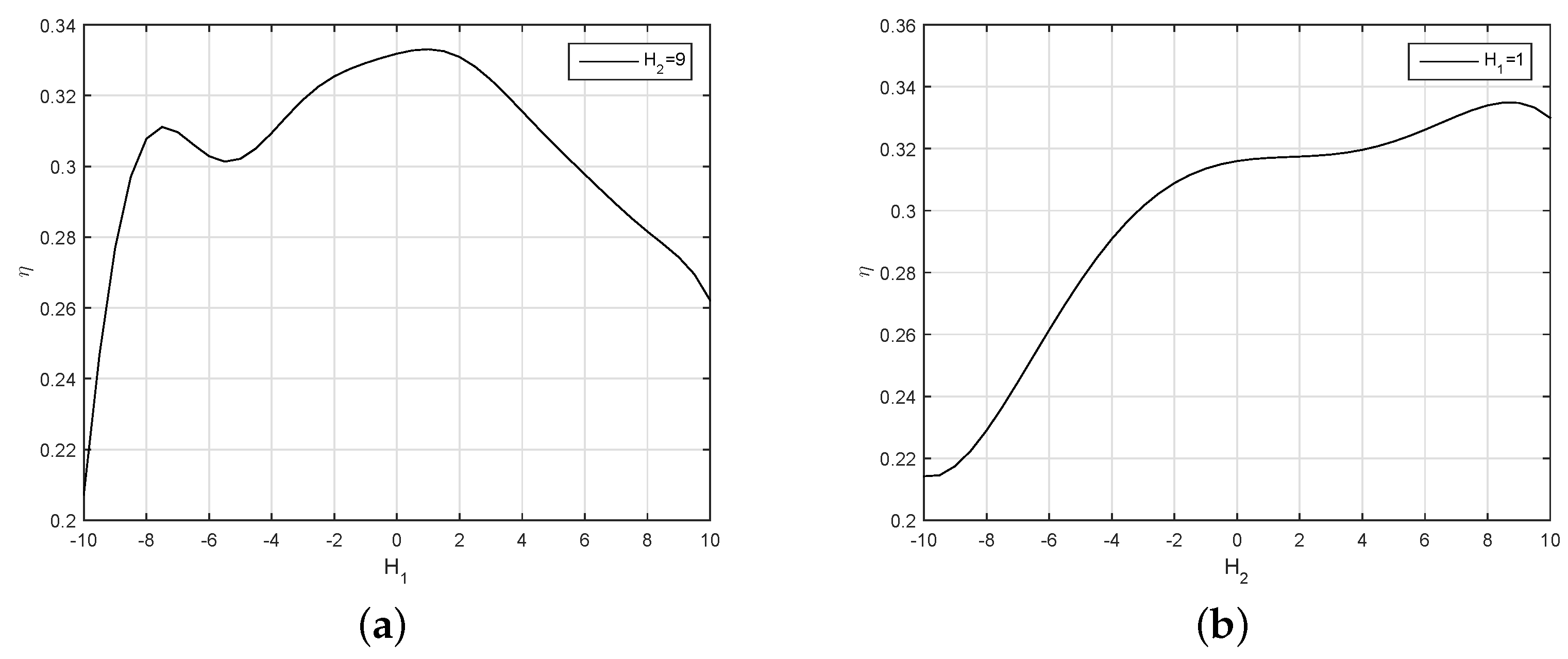
In Figure 16, when $K_2=16$, after reaching a maximum value at $K_1=5$, the efficiency of the robotic fish decreases to a minimum at $K_1=25$. Therefore, 5 is a good choice for $K_1$.

The results also show the changing of the efficiency along with the variation of $K_2$. The value of $\eta$ fluctuates with the change of $K_2$. We found that if the $K_2$ is too large during the simulation experiments, the curve will show a large overshoot, so we finally chose $K_2=16$.

Figure 17 depicts how the intensity of the feedback of the virtual spindle affects efficiency. The efficiency increases with the increase of $H_1$. $H_1$ is set to 1 for the intensity of the virtual spindle in the first joint. The relation between the efficiency and $H_2$ is an upward convex curve, which gets its maximum at $H_2=9$.

The virtual spindle model in VMM is the part to percept the force of the flow field onto the robotic fish and to add the adaptive response into the torques. The values of $H_1$ and $H_2$ have an obvious effect on the efficiency.

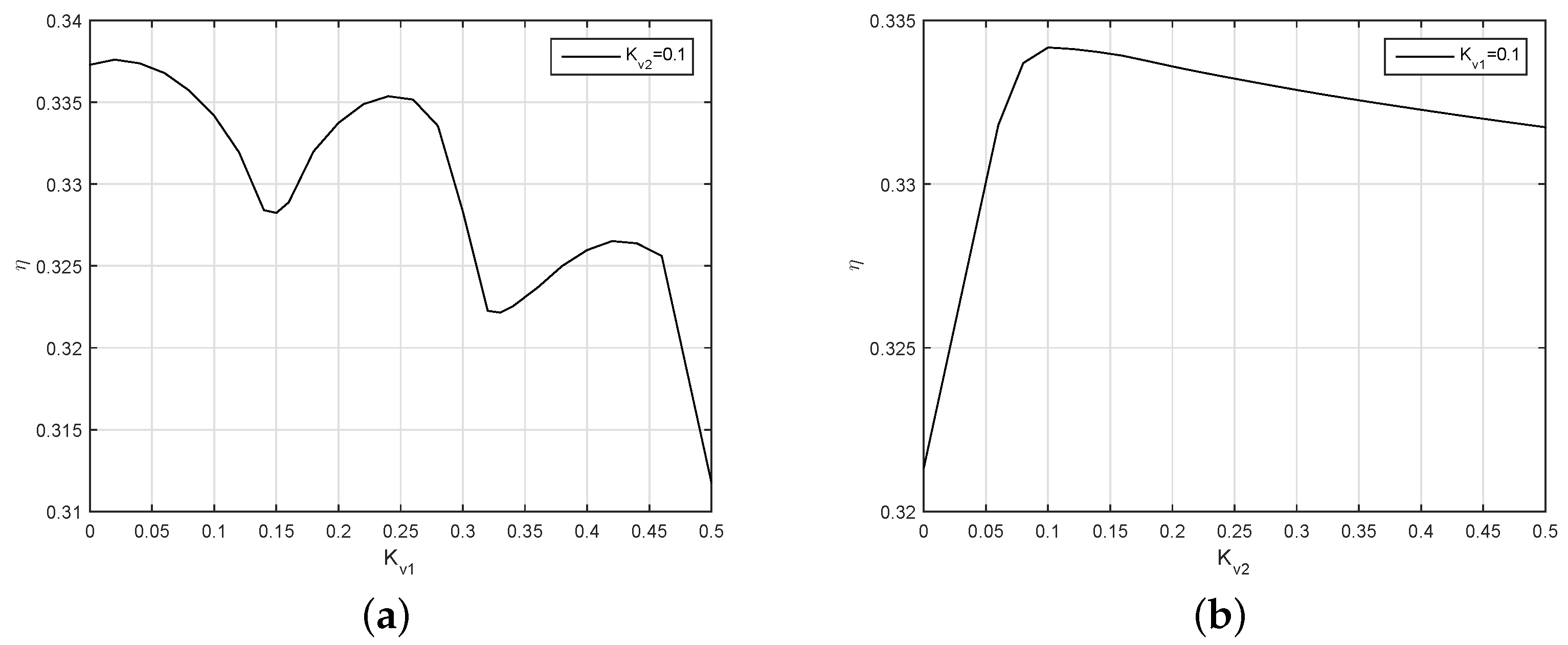
In Figure 18, the efficiency curve of the robotic fish fluctuates and decreases with the increase of $K_{v1}$. When $K_{v1}$ is less than $0.07$, though the efficiency is high, the robotic fish cannot follow the given speed. The gain is so small that the closed-loop control cannot eliminate the following deviation of the speed. To balance the swimming efficiency and the following of the closed-loop control, we chose $K_{v1}=0.1$. The efficiency to $K_{v2}$ is an upward projecting curve; it rises quickly before $K_{v2}=0.1$ and declines slowly after this point. At $K_{v2}=0.1$, the efficiency reaches its maximum value. Simultaneously, the swimming speed of the robotic fish is also in good condition.

5. Conclusions

In this paper, a novel closed-loop algorithm describing how to control the swimming efficiency of a robotic fish was proposed. We established the dynamic model and the hydrodynamic model of a two-joint robot fish. We formulated the problem of raising the propulsive efficiency as an algorithm designed in the joint space. Moreover, we characterized the mechanism of how the fish moves under the control and drive of the nerve and the muscles. Consequently, we abstracted a virtual musculoskeletal methodology from the nerve and muscle system and applied it in the joint space of the robotic fish. We evaluated the performance of the robotic fish controlled by two kinds of methods in the steady flow and Karman vortex. The results showed that the closed-loop control via virtual musculoskeletal methodology is more energy-efficient than the proportion control algorithm in both kinds of flow. The insight is that the virtual musculoskeletal methodology brings compliance to the muscles in the joints. Therefore, the robotic fish can adapt to the hydrodynamic effects of the water to reduce energy consumption when swimming.

In our future work, we will build up a more general swimming model of the robotic fish by considering complex flow turbulence to adapt to the real environment. Additionally, we will take the task planning into the closed-loop control for the applications. Finally, we will build up a real platform and conduct experiments on it to evaluate the performance of the proposed algorithm.