Remotely Controlled Robot Swarms: A Structural Analysis and Model for Structural Optimization

Abstract

In this paper, the authors analyse the structure of robot swarms. Drive, communication, and artificial intelligence technologies have reached a level where the inspiration of the animal world has become very useful for the development of systems of which people have dreamed for centuries. A short introduction describes the need for and expectations of autonomous robots and vehicles. A classification of swarm structures is based on animals such as bees or ants. Two main types of swarms are recognized: structural (master–slaves) and non-structural. The operator controls both of them remotely. The swarm structure has a great influence on the structure of single robots. A computer model with an object programming definition was worked out, and a simulation of the presented swarm structure is provided. The results are described in the paper.

1. Introduction

There is no doubt that robots will be a part of our future life, perhaps sooner than was assumed some years ago [1]. Robots are becoming more popular in factories due to the high costs of human labour forces [2,3]. Robots have become dominant in rescue services and have been introduced to armies as reconnaissance or fighting devices [4]. It is desirable to have intelligent slave robots that behave similarly to living creatures, except for their obedience to a master, even if this requires suicide. People have dreamed of machinery similar to live creatures, in appearance and behaviour, for many years. Thanks to progress in artificial intelligence and mechatronics technology, those dreams are becoming reality. Our expectations of robots are shaped more by science fiction and movies than by real needs. New types of humanoid or bionic robots have been developed over the last 40 years [5]. Robots can take on the appearance of live creatures, such as fish, kangaroos, dogs, etc. Together with their mechatronic control system, robots’ mechanical construction enables them to perform very complicated movements, such as running, jumping over obstacles, and even some acrobatics. Such robots are the top of the line. However, most people use robots for simpler duties, such as transport, cleaning, etc. For such work, one of the crucial problems is embedding into the robot body the intelligence needed for navigation and movement trajectory planning.

A swarm is a group of identical creatures that look, move, and behave in a similar way. However, the swarm as a whole has a visible or invisible structure and moves and acts in accordance with certain rules. For instance, a swarm can consist of intelligent creatures or robots that maintain a set distance from each other, which creates the group intelligence required for the creatures to move and act together. The basic element of a robot swarm is a robot [6,7].

Swarms have played an important role in the history of the development of species. We can see that many species have survived thanks to teamwork or living in a swarm. Weak creatures can work together as a swarm to defeat a much stronger enemy.

The main scientific problem we address here is how to effectively control a robot swarm, especially during simultaneous movement to a destination and given the individual actions of all robots. The important scientific question is how to create swarm intelligence, even for primitive creatures.

If we understand swarm rules, we will be able to build low-cost robots (or unmanned aerial vehicles (UAVs), or ground unmanned vehicles (GUVs), popularly called drones) for the realization of large-area tasks, such as searching for people under building ruins avalanches, looking for and neutralizing contamination, etc. We can imagine many tasks that need to be accomplished quickly over a large area, which many simple robots could do more quickly than a few more advanced ones. The control of a robot swarm is a huge problem, because each robot moves individually, with different coordinates [6,8].

Robots acting in a swarm will play an important role in defence systems in the protection against enemies [9]. It is expected that a swarm of cheap robots would be more effective and fault-tolerant than expensive individual robots.

As the swarm occupies a large area, it is possible that it will meet some obstacles on its way. A swarm can evade an obstacle while maintaining its structure as one rigid body—without space between the robots—so long as all robots avoid it on the same side. This can be time- and energy-consuming. When we observe an animal swarm, we notice their ability to change the swarm’s structure in order to avoid obstacles, even though the individual animal may seem quite primitive [10]. Some animals living in a swarm die when they are outside of it. We can conclude that swarm intelligence is required to split and reconfigure itself. The research problem in the current study is the question of what is required in order to create an intelligent swarm of robots.

Currently, mobile robots are intelligent enough to provide self-navigation, which means travelling in a programmed path with small route corrections caused by obstacle detection. A higher level of intelligence involves finding the way based on the robot’s current position and destination. Others navigate based on smell, vibrations, or air movements. For this study, a remote control signal generated by an operator simulated other steering signals.

The intermediate solution is a remote control system supported by an operator who observes the robot and changes the movement direction. The robot has to be equipped with a remote control system added to the drive system and obstacle detection to avoid crashes. In the air, navigation is much easier than on the ground, where obstacles can be met [11].

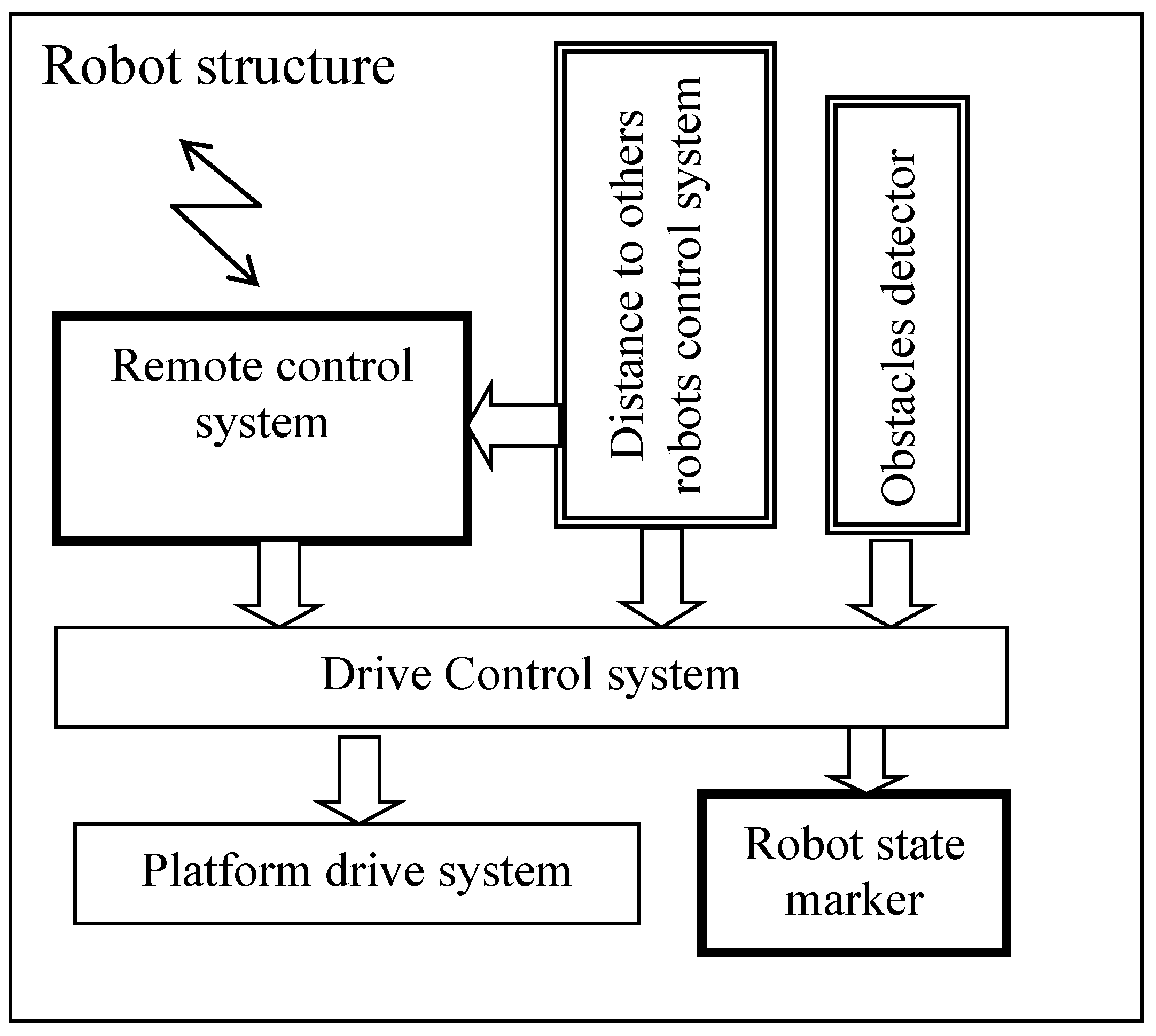
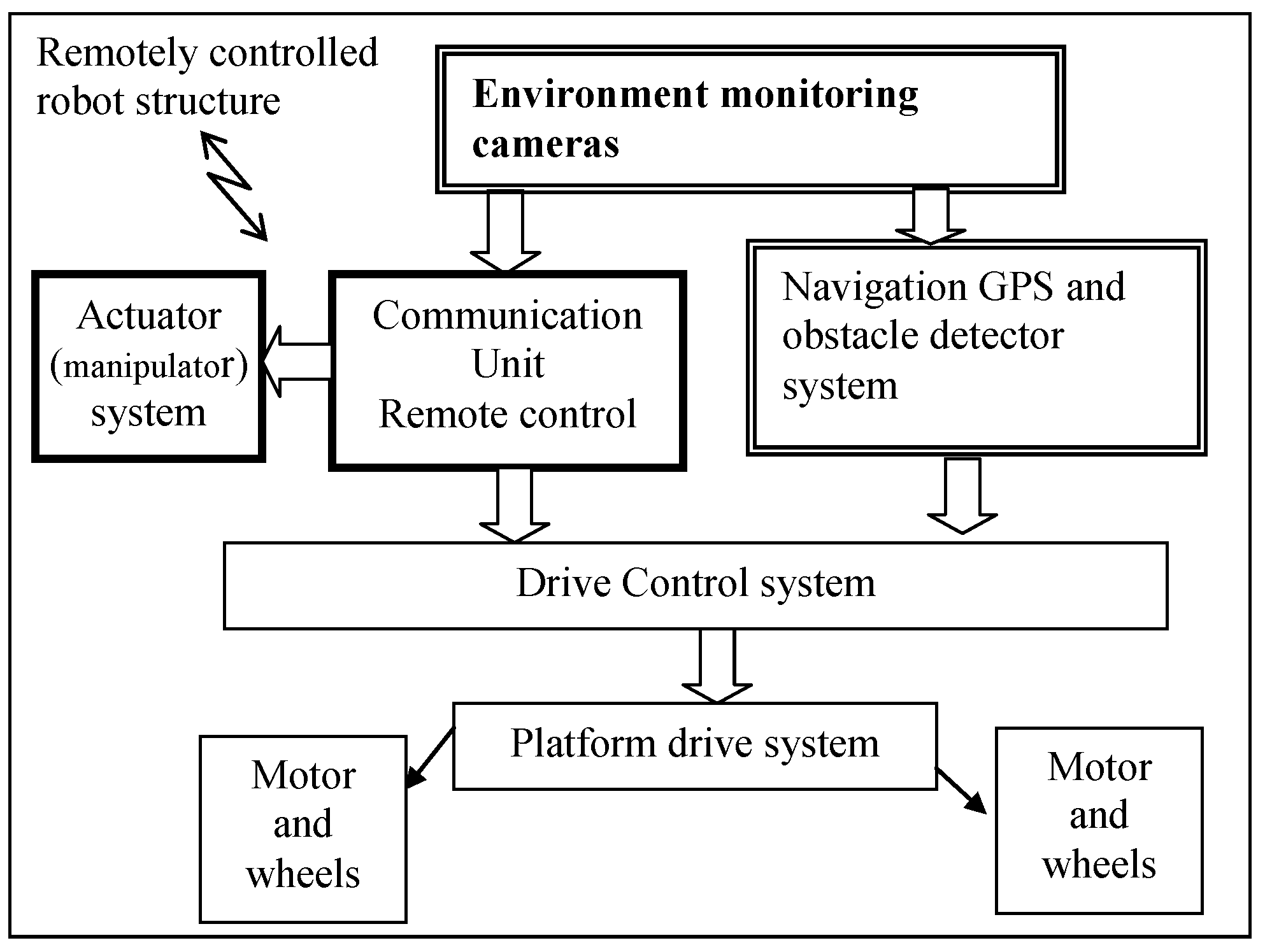
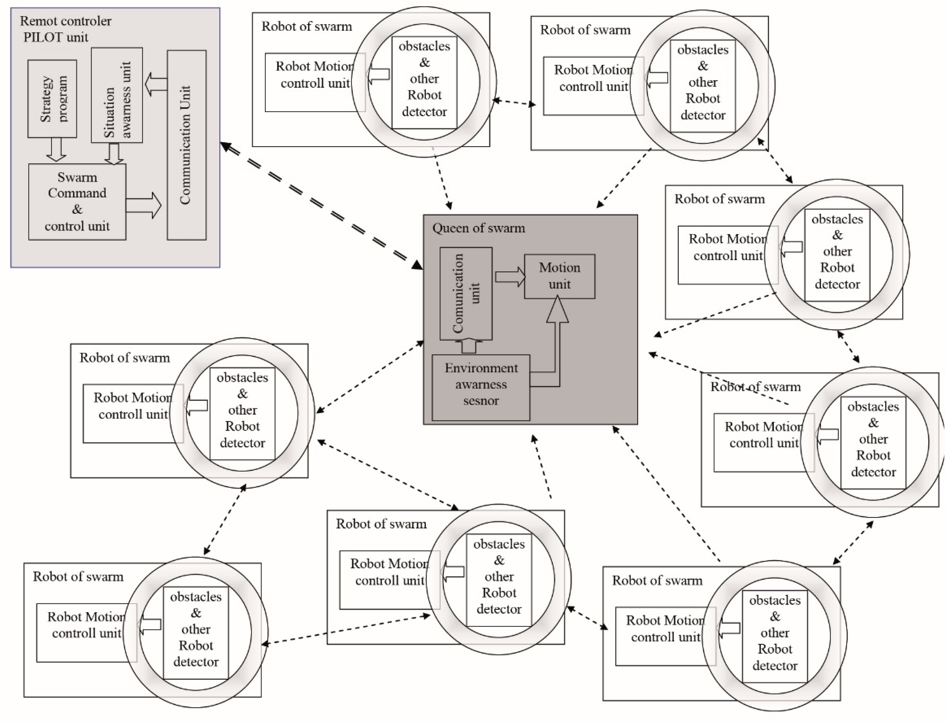
The operator has to be awarene of the current situation, which can be achieved by using a camera mounted on the robot or an external observatory [12]. The basic robot system consists of:

• A ground-driven platform
• A navigation system with obstacle detectors
• An actuator—a detector used in the searching system
• A control system
• A situational awareness system (with commonly used cameras)

The model of the basic structure is presented in Figure 1.

Currently, many kinds of driven platforms are available. The navigation system is much more complicated, although many types of obstacle detectors can be used. In some applications, such as path finding in a labyrinth, separate obstacle detectors can be omitted because they can be replaced by a driving algorithm. When a robot meets a wall, the resistance to movement and the motor’s current increase rapidly, and the control system changes the movement direction in ta planned or random direction [13].

When a robot is controlled by an operator, s/he can observe its movement and lead it into a free space close to the assumed path.

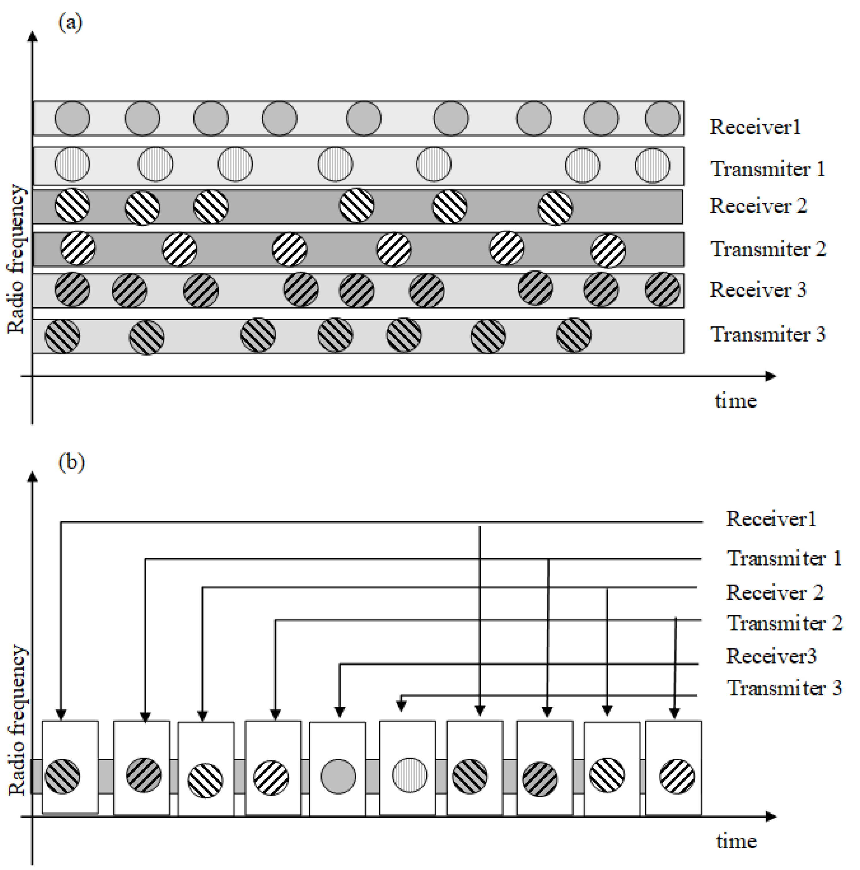
Current state of remote control systems. Usually, we use radio remote control devices. A radio frequency-coded signal is received and interpreted by radio-controlled devices, which pass the steering signal to the driving system. This is simple when a radio frequency (RF) control system is used only for one robot that is controlled with one frequency band.

If we use a few robots working in the same band, they might disturb each other’s signals, so we need as many separate frequency bands as we have robots. This is known as the frequency division multiple access (FDMA) technique. Another method of data exchange between a few transmitters and receivers is time division multiple access (TDMA). In this method, each transmitter–receiver pair works in the same frequency band, but they each have a separate and dedicated time period for the data exchange. Both techniques can be found in drones that are available for purchase on the Internet or in supermarkets. Examples and differences between the FDMA and TDMA systems are presented in Figure 2 [14].

When a few robots have to be controlled separately at the same time, many operators are needed [15]. As the number of robots increases, so does the number of operators needed. A problem appears when we try to control a swarm of robots. It is very difficult to control all robots separately. When robots are in an action area, they work individually, according to programmed algorithms, after receiving the command to start the programmed mission. Moving all robots from place to place can be much more complicated if there is an obstacle to avoid. It would be useful if an operator could control all the robots as a whole. The adequate structure for such control requirements would be a swarm, which can be controlled as one body, and which transforms its shape to avoid obstacles. The individual robots would choose their path to avoid obstacles but try to keep themselves in a swarm structure [8].

The main scientific and technical problem in this study was how to find the simplest structure of a robot that can cooperate with other robots in a swarm. The scientific questions were: what is the simplest structure of a swarm member, and how is the intelligence of the swarm created? Is the swarm more or less intelligent than the most or least intelligent member of the swarm?

The hypotheses of this study were that:

• It is possible to control all the robots in a swarm as one (flexible and penetrable) body.
• The cloud of robots can feature swarm self-organization skills similar to animals’ swarm intelligence.
• The intelligence of a swarm is higher than that of any individual member of it.

To prove these hypotheses, analyses of the chosen swarm structure were performed (Figure 3). Computer models of swarms with a small number of members were created and investigated with real model tests. Next, more complicated structures were analysed and modelled. In this study, the authors focused on movement strategy, not on decisions about movement direction. In the natural world, the signals for movement could be smell, acoustic signal, light, etc. For robots, it was supposed that a remote control signal would be enough.

2. Materials and Methods

The methods were based on analyses of existing systems in the human and animal world, including hierarchical and non-hierarchical structures. These systems can be converted into robot structures [16]. However, we met with some difficulties in following natural systems, so some simplifications and substitute solutions were found.

Swarm structure and movement strategy analyses could start from the bottom, with insects, or from the top, with humans, e.g., soldiers in formation. The former has no visible structure and its members work together according to unknown rules. The latter has a clearly defined structure and rules of movement. Between them we have semi-structured swarms, such as bees, etc. Swarms with a reconfigured structure have also been identified [16], which we also took into account.

During the literature review, we found more questions than answers about insect behaviour and how it can be transferred to the robot world; instead, therefore, we started with the most advanced structure. Initially, the hierarchical swarm model was built based on soldier formation movement in a matrix. Although it consisted of the most intelligent creatures, it was the easiest to analyse because the authors are experienced in military service. Therefore, it was easy to build a logical model and an algorithm for swarm behaviour. For these analyses, some typical scenarios were prepared. These scenarios described the movement conditions and required paths. These movements were planned to be performed in a straight line and in curves, in various formations, such as in single file or in a matrix. The algorithm for an individual robot’s movement depended on its role in the swarm. Its task was to maintain its position in the swarm. In various scenarios, the formation was changed. During algorithm building, the information needed for robot and drive skills was defined. This information was delivered with control signals or by sensors.

For such structural and logical models, relevant computer models were built. These models consisted of an environment model, a model for each robot (depending on its role in the swarm), and a command system. The non-homogeneous environment introduced some randomness into the process. Furthermore, the static distribution of robot parameters was introduced. In some scenarios, the failures of some robots were modelled to check the robustness of the swarm. Simulations were repeated a few times (for a changed environment or a new robot setting in the swarm), recording the path of each robot. After each simulation, the results were analysed and discussed. If everything was proceeding in the assumed way, the structure and logicical algorithm of the robot were simplified. If not, the structure was improved. However, the method was directed towards the simplification of the structure in order to make it more similar to that of insects—a non-hierarchical, homogeneous swarm structure.

For the purpose of verification, a swarm of five robots was used. The robots were built on a platform consisting of a remotely controlled electric vehicle with a modified driving control system and an added microcomputer module with sensors. These modules were from Arduino and featured a ultrasonic distance sensors; the others had a specially designed optoelectronic module with a camera and lighting markers.

For a structural swarm, only one robot—the leader—received the control signal, and moved according to it. For a non-structural, homogeneous swarm, all the robots (using the same RF band) received and followed this signal.

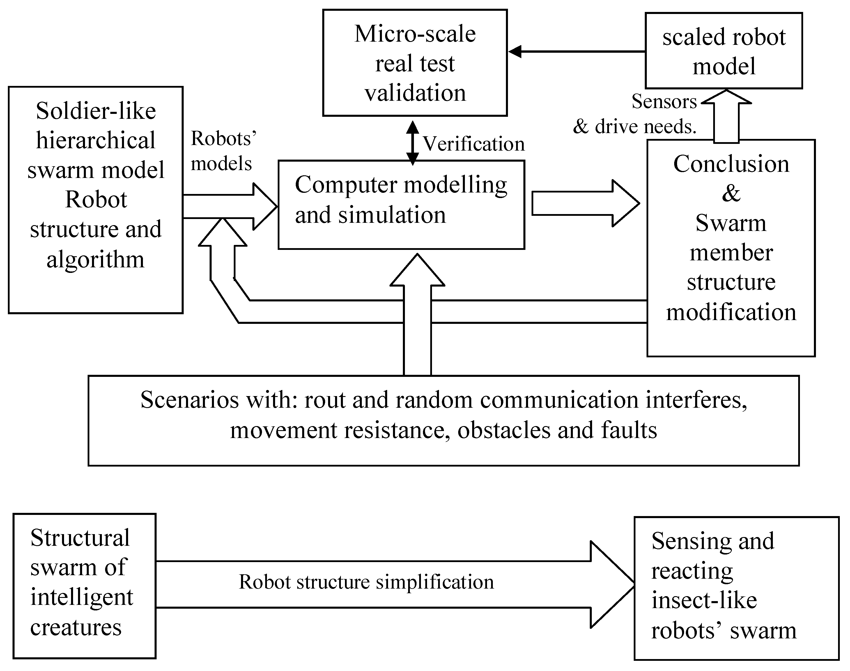
The main goal of this work was to determine the optimal structure of a robot, with the sensors and algorithms required in order to create the most effective swarm during motion on a required path.

The starting point was the model of a soldier-like structural swarm. This model was verified with a computer model and real tests with simple scenarios. In the next steps, the model of the individual robot was simplified and homogenised. Each model was tested by a simulation. Some elements of the scenarios and simulation results were validated by real tests. The process consisted of many iterations.

2.1. Scenarios and Analyses

A group of soldiers is a hierarchical structure featuring a superior and subordinates. The commander leads the team. The team moves in an array formation (rows and columns) [17]. The members try to stay at a particular distance from their neighbours in front and to the side, and to stay in a line. However, those in the first row only have one person ahead of them—the leader—who should be in the centre, at the front. A robot’s position in the array is fixed. During turning, the robots have to adjust their speed in order to keep in line. Finding the algorithm for such an action is not difficult, but we needed quite a complicated sensor system with actual state evaluation. For the next simulation, if one of robot fail, the formation matrix needed to be reconfigured. In other words, the robot needed to be ready to change its position and algorithm of action. The potential for error applies to all robots, including the leader. If any robot can play any role, then all of them have to be equally advanced. Paradoxically, the leader can be prepared for only one role. For a hierarchical swarm, we assumed that its structure would be reconfigurable during movement, that obstacles would be avoided by the leader, and that the others would follow suit.

2.2. Simulation Program

The investigation was performed through computer simulations, which were partly validated by experiments. The simulation program was prepared using Delphi object software (see Appendix A). Each robot was modelled as an object. The structure of the object depended on the swarm structure and on the role of the robot in the swarm. The field in which the robots moved was modelled as a 2D array of records: the movement resistance value, determined by the array coordinates on hexagons on the ground; and the state of occupancy of the hexagon by a robot or field.

The field of simulated action was divided into hexagons in order to speed up the simulation process, because the shape of a piece of field was similar to a circuit and made it easier to detect the distance between the robots.

The values could be constant or change over time.

The results of the simulations were displayed as a sequence of robot positions on the field. The robots were traced using a path, which was compared with their assumed path. The robots were represented by circles of different colours, marking their roles in the swarm.

The robot’s position was calculated as the value of the integrator versus the time of its speed vector components.

Generally, it is assumed that robots in a swarm keep their distance from one another within a defined range. When robots move, their speed is decreased when their distance to another robot in the movement direction is too small, or increased when the distance grows.

The simulation was based on a few scenarios that involved running through the test field on a determined path. The operator controlled the swarm’s movement with keyboard arrows, as in a video game. One of the study problems was developing a swarm that was tolerant of failures, e.g., a loss of radio connectivity, a breakdown, or the loss of a few members.

2.3. Relative Position Sensors

For the simulation, a robot model was created. It consisted of a state optical signaller, its distance from robots and obstacles, equipment, and a driving system.

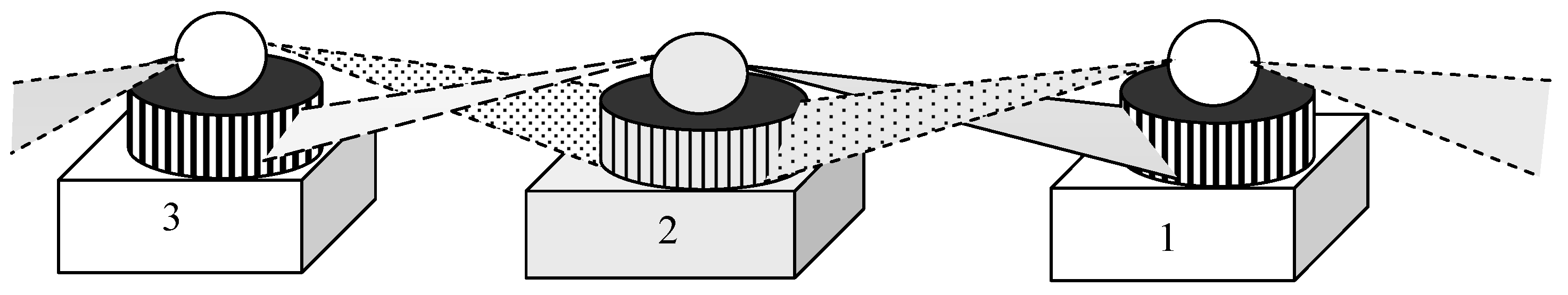
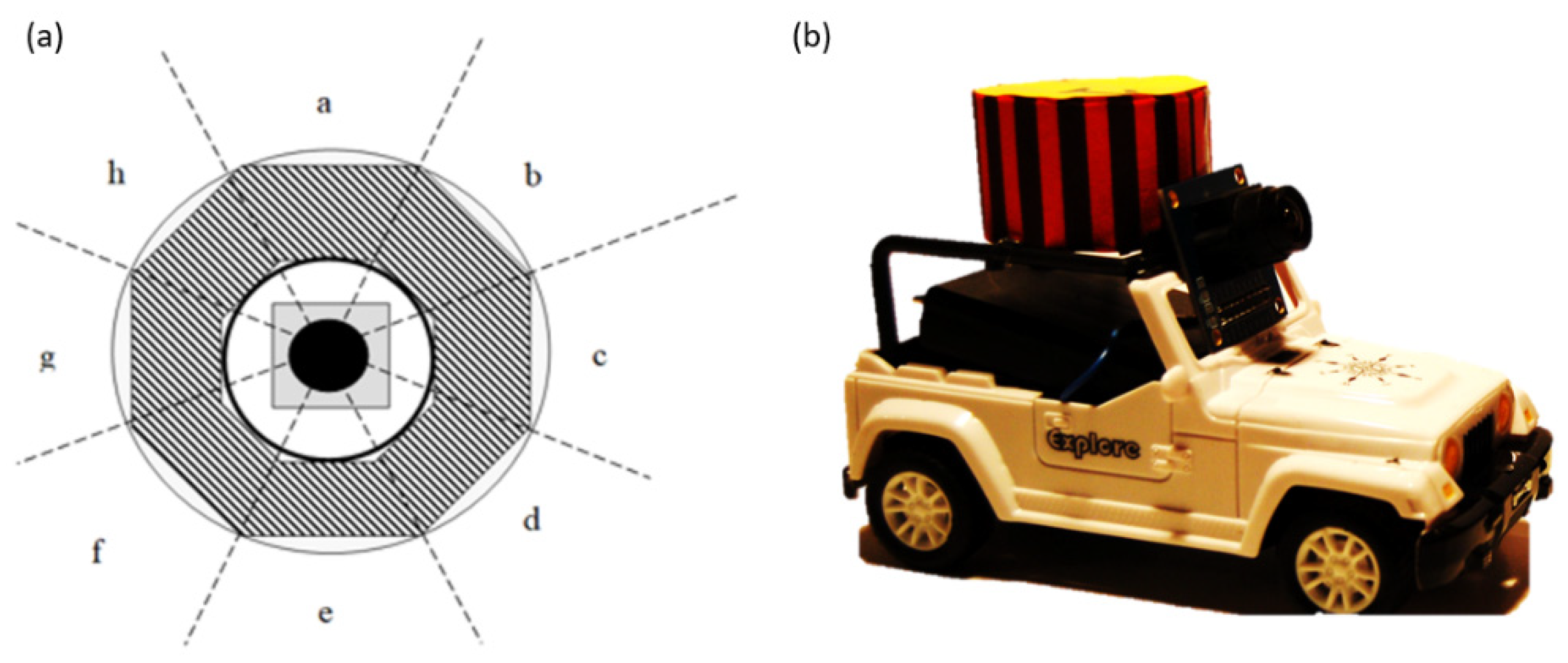
The signaller was an optical marker in the shape of a lighting cylinder, as shown in Figure 4. The signaller featured a defined dimension so the distance to it could be evaluated based on the angle of sight (the length of the mark seen in the picture) of a camera. If a robot was out of order, the light switched off and it was treated as an obstacle. Using different colours or flashing light frequencies, the role or dedicated position of a robot in a swarm could be coded and recognized.

The robots’ distance from obstacles (and other robots) was measured with ultrasonic sensors located around the robot at 45°, as shown in Figure 5. For this, a computer model was used, so the ultrasonic sensors did not interfere with each other. In the real built model, ultrasonic frequencies and optical (camera) analysis were used.

2.4. Driving System and Distance Control Model

The driving system was responsible for the speed and direction of the robots’ movement. The required robot speed and direction were remotely controlled, and modified based on the robots’ distances from other robots and obstacles, according to the implemented algorithms. Moreover, the driving system was a model with a changing maximum speed limit. The limit depended on the energy used in the previous period of movement. The required speed depended on the robots’ distance from other robots in the follower model, or on these distances and the commanded speed in the unstructured swarm.

The swarm was modelled with N two-dimensional columns and a two-row matrix, where N is the number of robots in the swarm, and two dimensions, X and Y, were used for positioning:

$$\left[\begin{array}{c}{X}_1\\ Y_1\end{array}\begin{array}{c}{X}_2\\ Y_2\end{array}\begin{array}{c}\cdots \\ \cdots \end{array}\begin{array}{c}{X}_N\\ Y_N\end{array}\right]$$

(1)

The position of a robot is a vector [X,Y], calculated according to Equations (2) and (3) for each column of the above matrix:

$$X_n=X_{0n}+{\displaystyle \sum }{V}_{xn}·\tau =X_{0n}+{\displaystyle \sum }{V}_n·\tau ·cos{\alpha }_n$$

(2)

$$Y_n=Y_{0n}+{\displaystyle \sum }{V}_{yn}·\tau =Y_{0n}+{\displaystyle \sum }{V}_n·\tau ·sin{\alpha }_n$$

(3)

where τ—the integration time interval.

X_0n, Y_0n—the initial position of n robot in the absolute coordinates system

V_xn, V_yn—the speed vector components in the absolute coordinates system

V_n—the robots’ movement speed

α_n—the direction of movement

The required speed of movement was calculated according to the following rules.

In a structural swarm model:

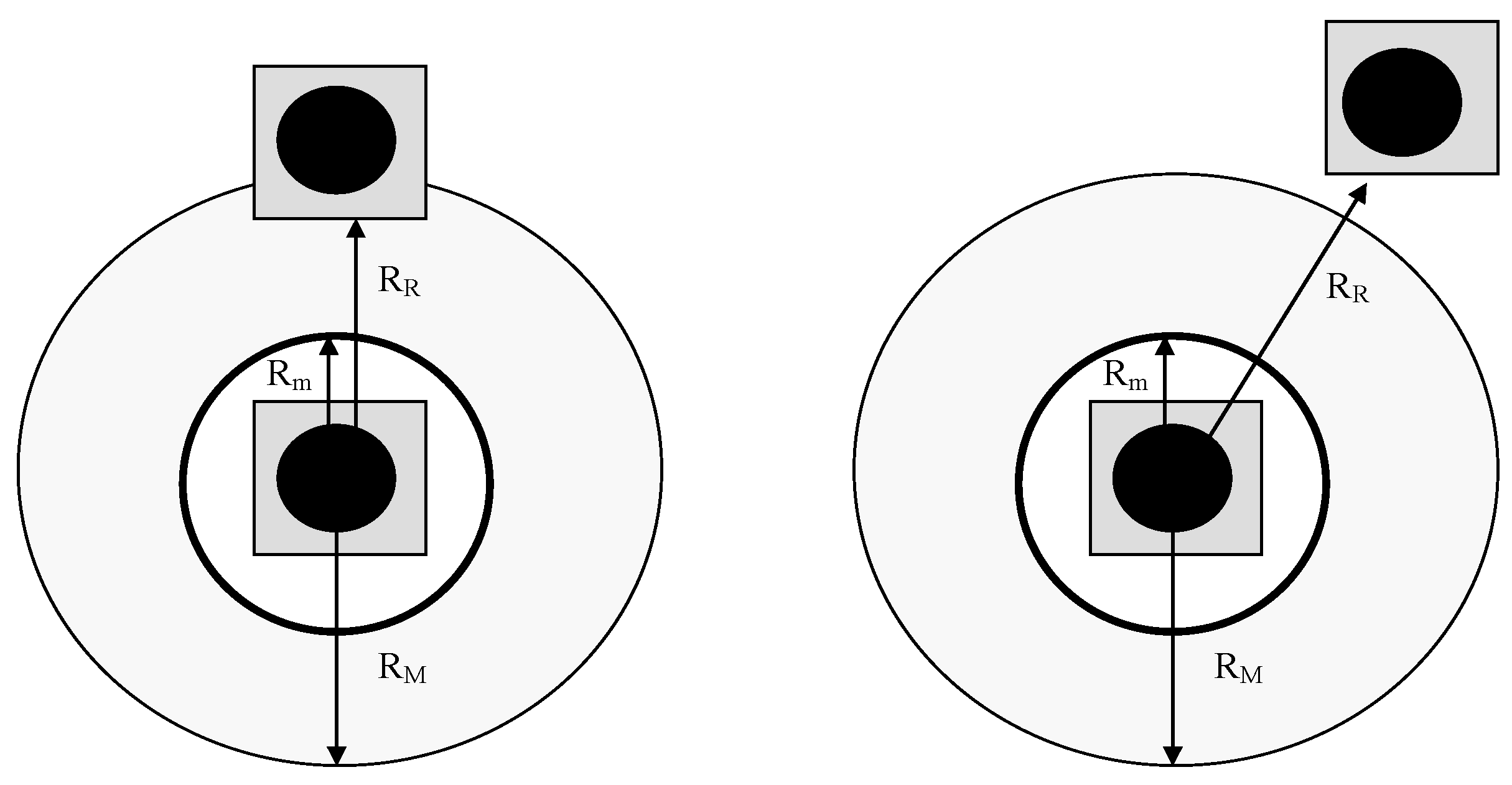
In the first modelling approach, the required speed V_zF is proportional to the difference between the real distance R_R to the predecessor and the minimal assumed value Rm, as shown in Figure 6:

This is the limited (saturated) P regulator model:

$$V{z}_F=k_{VZ}\left(R_R-R_m\right)$$

(4)

$$Vz=\{\begin{array}{l}V{z}_F,\hspace{1em}|\hspace{1em}V{z}_F<VL\\ VL,\hspace{1em}\hspace{1em}\hspace{1em}V{z}_F\ge VL\end{array}$$

(5)

where k_VZ is the magnification of the proportional speed regulator. If R_R is lower than R_m, the required speed is zero. However, the real V_r speed of movement depends on movement resistance M, so it can be modelled as

$$V_r=Vz-K_{M}M$$

(6)

The M value is generated by a random value generator (rand(t)), giving a value in the range 0–1, and the MA is the maximum resistance.

$$M=MA· rand\left(t\right)$$

(7)

The real speed cannot be higher than the speed limit VL, which depends on the energy source wearing out:

$$VL=VL0-KL{\displaystyle \sum }M\tau$$

(8)

This wearing out depends on the movement resistance on the way and the wearing-out coefficient KL.

In the second approach, the distance from the followers is taken into account, which makes the VL0 lower.

$$V{L}_R=k{L}_{VZ}\left(R_M-R_r\right)$$

(9)

When the robots are not moving in line, the angle α (turning) is calculated based on the difference between the central position of the predecessor and the robots’ distance from it.

When an unstructured swarm was considered, the speed in two dimensions was calculated in a similar way.

The upper and lower speed limits in both directions were calculated for the distance between the robots, keeping them within the assumed range. If the remotely ordered speed was in a limited range, then it was executed.

For an unstructured robot swarm, the distance between the robots was given higher priority than the required speed (value and direction).

The other regulator used was a model with hysteresis, or a death zone. If the distances between the robots were within the zone between Rm and RM, the required speed could be calculated as follows:

$$V{z}_n=\{\begin{array}{l}V{z}_{n-1}-k_{vz}{\left(R_r-R_m\right)}_{},\hspace{1em}|\hspace{1em}{R}_r<R_m\\ V{z}_{n-1}+k_{vz}\left(R_M-R_r\right),\hspace{1em}\hspace{1em}{R}_r\ge R_M\end{array}$$

(10)

In this case, the speed limit was also applicable:

$$V{z}_n=\{\begin{array}{l}V{z}_n,\hspace{1em}|\hspace{1em}V{z}_n<VL\\ VL,\hspace{1em}\hspace{1em}V{z}_n\ge VL\end{array}$$

(11)

3. Results

The analyses of the swarm structure was based on human team actions and insect swarm actions.

3.1. The Analysis of Human and Insect Swarm Patterns as a Reference for Robots’ Swarm Structures

A human team of soldiers and insect swarms were chosen for the analyses, as examples of the most and least advanced group structures.

A group of soldiers is a hierarchical structure featuring a superior and subordinates. The commander knows the team’s task and plans the role of each member of the team. The team moves in an array formation (rows and columns) [17]. In this model, the front (first) row is followed by the second, and so on; each row tryies to walk in the previous row’s footsteps. The distance between members is kept at an almost constant value. The members in the next row follow the previous one in their columns. The problem is how to keep the alignment of the rows, so the leader needs to be an example to the front row. The array is set, and the positions of its members are not changeable. During turning, the speeds of soldiers in a row are different and controlled by themselves in reference to their neighbours. A robot in a line has to pay attention to the robot ahead of it in the column, but in the first row the robots’ consideration is their distance from the leader and from the other robots in the row. This is not easy, even for human soldiers who are specially trained for it. For such scenarios of movement, we have various functions in the array: the leader, the first row member, and the followers.

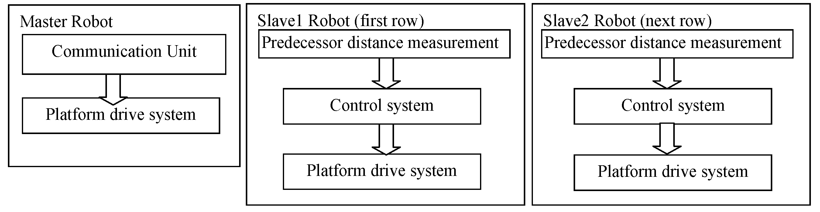
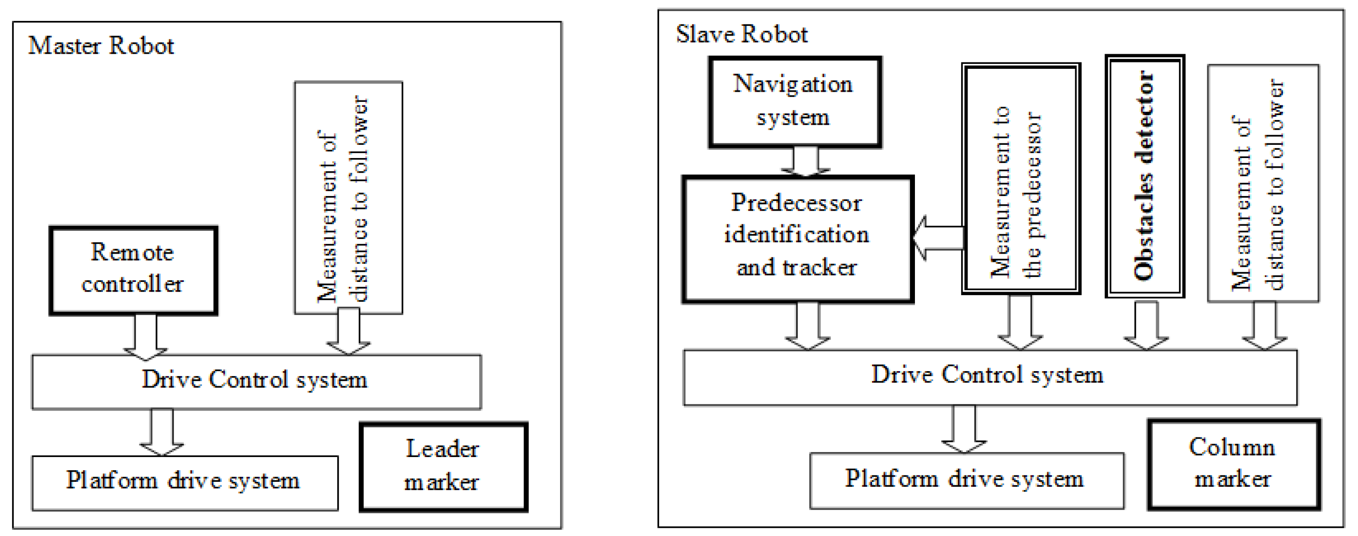
Therefore, we designed three roles for the robots (Figure 7):

• The commander, which can be remotely controlled (Master).
• The member of the first row who keeps an eye on the position of the commander and follows in line (Slave 1).
• The follower who is behind the first row and maintains a set distance from the robot ahead (Slave 2).

For robot teams riding through a field, keeping in a straight line is not important in many cases. The simplification of only needing to maintain precise distances between the robots within a column can be effected.

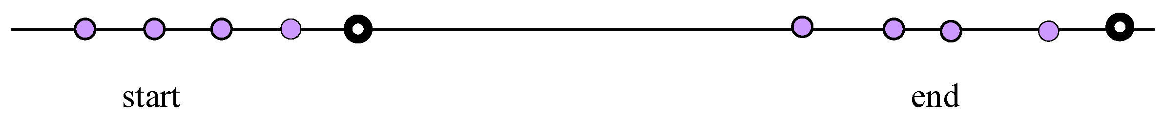
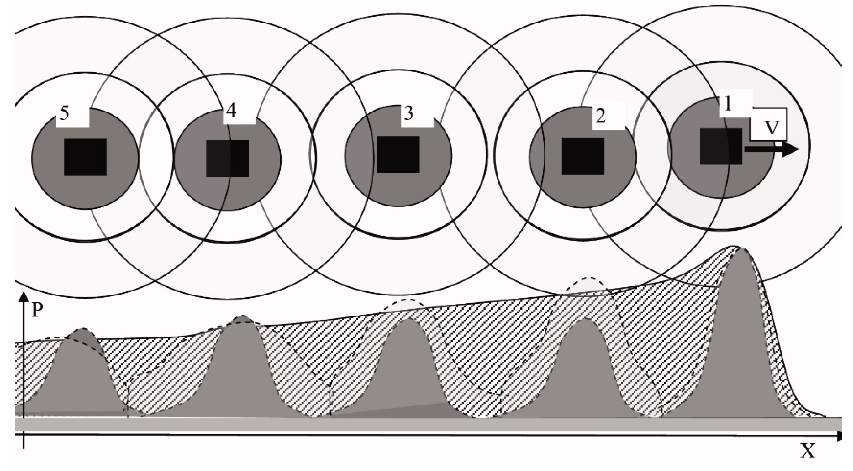
A simulation of robot column movement was performed (Figure 8). This simulation involved similar problems to those involved in vehicle platooning. When the leader moved in a straight line, because of various types of resistance, its speed changed. The follower tried to maintain the distance between them by slowing down or speeding up. Due to inertia, this took time, so the distance changed. In the process of distance control, the variability of the motion resistance also applied to the successors. Thus, the actual speed of a given robot was an effect of the instability of its predecessor and its own speed.

The farther the robot is from the leader, the more random the speed is, as a result of the many components involved. This is shown in Figure 8. Moreover, when we included the robots’ speed, we observed that the distance between them grew. As a result, we could only define leader’s position, while the other positions were random. If the distance between robots increases too much, the line may break. Therefore, in order to maintain the line, we needed to control the distance between the leader and the followers, giving higher priority to the distance to the robot behind. Consequently, all the robots moved at a speed no higher than that of the slowest robot. To mitigate this problem, the followers should have a reserve of power to overcome resistance without decreasing their speed and for quick compensation for the growing distance.

Variable speeds solved the problem of straight movement. When the leader turned, the followers had to control their position within a certain range of angles. When the leader turned, the follower followed according to the shortest possible path, rather than by simply repeating the leader’s path, as shown in Figure 9.

In an array, the follower has to control the distance to the robots at its sides in order to avoid interference. During many simulations with sinusoidal paths, the robots mixed up their columns. To help each robot follow the right predecessor, a distinction between the columns was introduced. An additional field was introduced and marked: the column number. In order to build a system based on a human array, the robots in each column should move according to the same path. The robots must not only maintain their distance from each other, but also follow their predecessors, so they need to observe and record the path and repeat it by respecting distance and keeping in line.

A human column can change its shape on command. This option is needed for robots as well. Robots should have built-in algorithms for transportation, and a defined position for all structures. If a swarm loses a member, the next robot in the column should take its place, moving to the front.

3.1.1. Summary of Structure Analyses

The robots were equipped beyond the assumed structure (presented in Figure 10) with:

• A distance-keeping system in the column (the distance of each robot from its predecessor and follower was in a declared range).
• The distance from the side robot controller.
• A predecessor track tracer.
• A column number marker.
• A remote control system for the leader.

The structures of the Slave 1 and Slave 2 robots were the same; the difference was in the software.

3.1.2. Results of Simulations

A few trajectory scenarios were tested. Those that had the greatest effect on the robots structure are listed below:

Action 1: The required path was straight in front of the leader. A random obstacle was placed on the road. For the first simulation, the swarm was set to one column; for subsequent simulations there were two, three, and four columns, respectively.

Results: The path in the simulation was similar to what was expected, but the array was spread out and the line was disturbed (see Figure 11).

Effects: A controller for the distance between the robots was introduced. To maintain the dynamics of the swarm, the robots needed a power reserve. As the lineup of the rows was not important, this result was acceptable.

Action 2: In the second simulation, an obstacle appeared on one side, but the leader moved in a straight line.

Results: The swarm avoided the obstacle as one.

Effects: A problem appeared in the first row, which was programmed to have the leader at its centre. This was resolved by adding a function for maintaining the distance from followers and the centrality of the leader’s position.

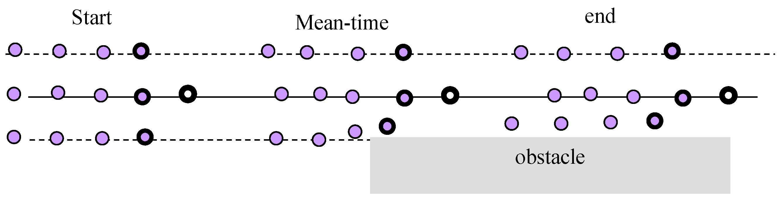
Action 3: The array structures passed between two walls, which forced them to compress.

Results: Fortunately, the movement of the robots from the side to the centre took time, so the central columns moved forward to the side, and some free space appeared for the robots in the side columns. The reconfiguration of the swarm took place by introducing the robots from the side columns between the robots of the central columns, as presented in Figure 12. After the robots passed the obstacles, the distance between the columns grew.

Effect: The algorithm forced the robots to stay close to the central columns when obstacles were detected.

The swarm will move in order if the algorithm controlling the distance between the predecessor and follower is flexible and based on information about the swarm reconfiguration.

Action 4: The leader turned and one column of robots followed it. The test was performed for one and three columns.

Results: If the robot did not have a predecessor tracking system, it followed its precursor via the shortest route, changing the trajectory of the swarm, as presented in Figure 13. Additionally, if the robots were not equipped with a tracking system to maintain distance, the followers took the shortest path. If an obstacle entered the line of contact, the robot needed to avoid the obstacle by moving in a different direction and, after passing the obstacle, searching for its predecessor.

Effect: The predecessor’s tracking system needs, track memory, and a global navigation system.

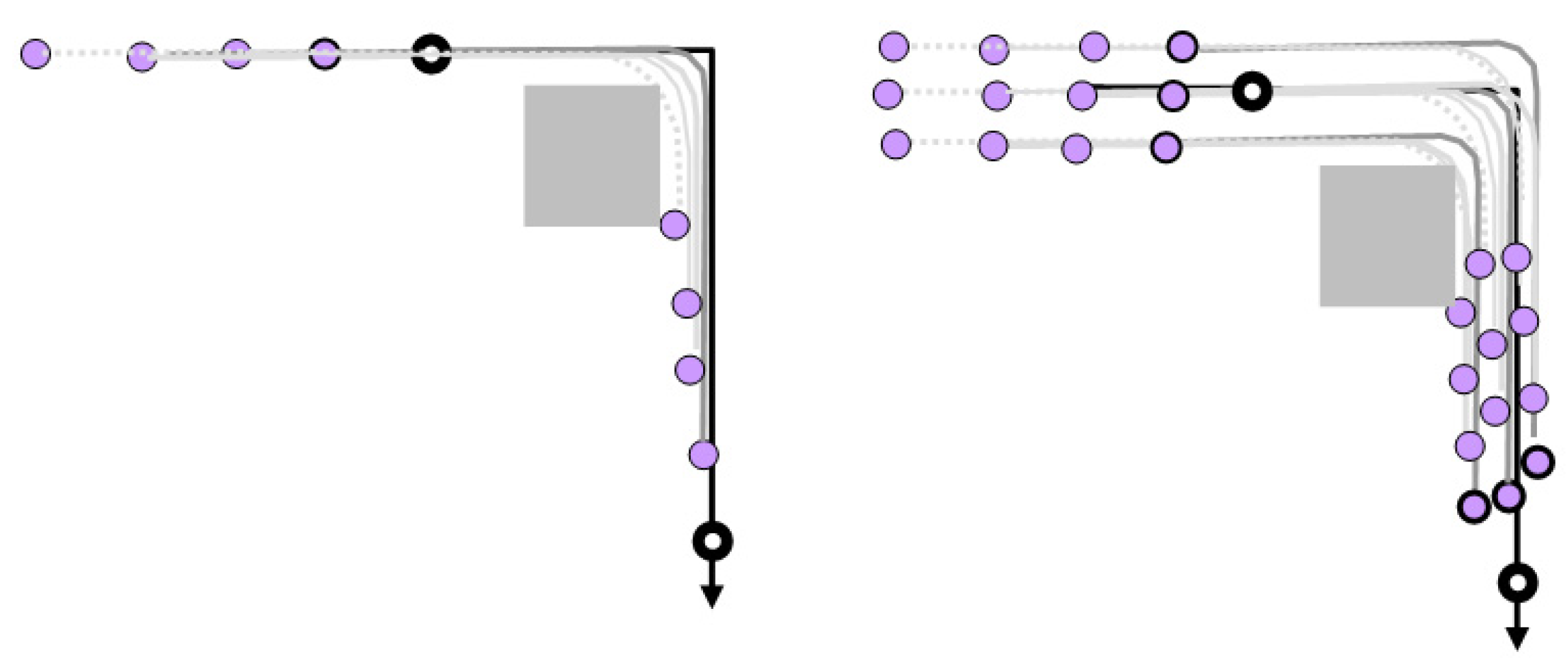
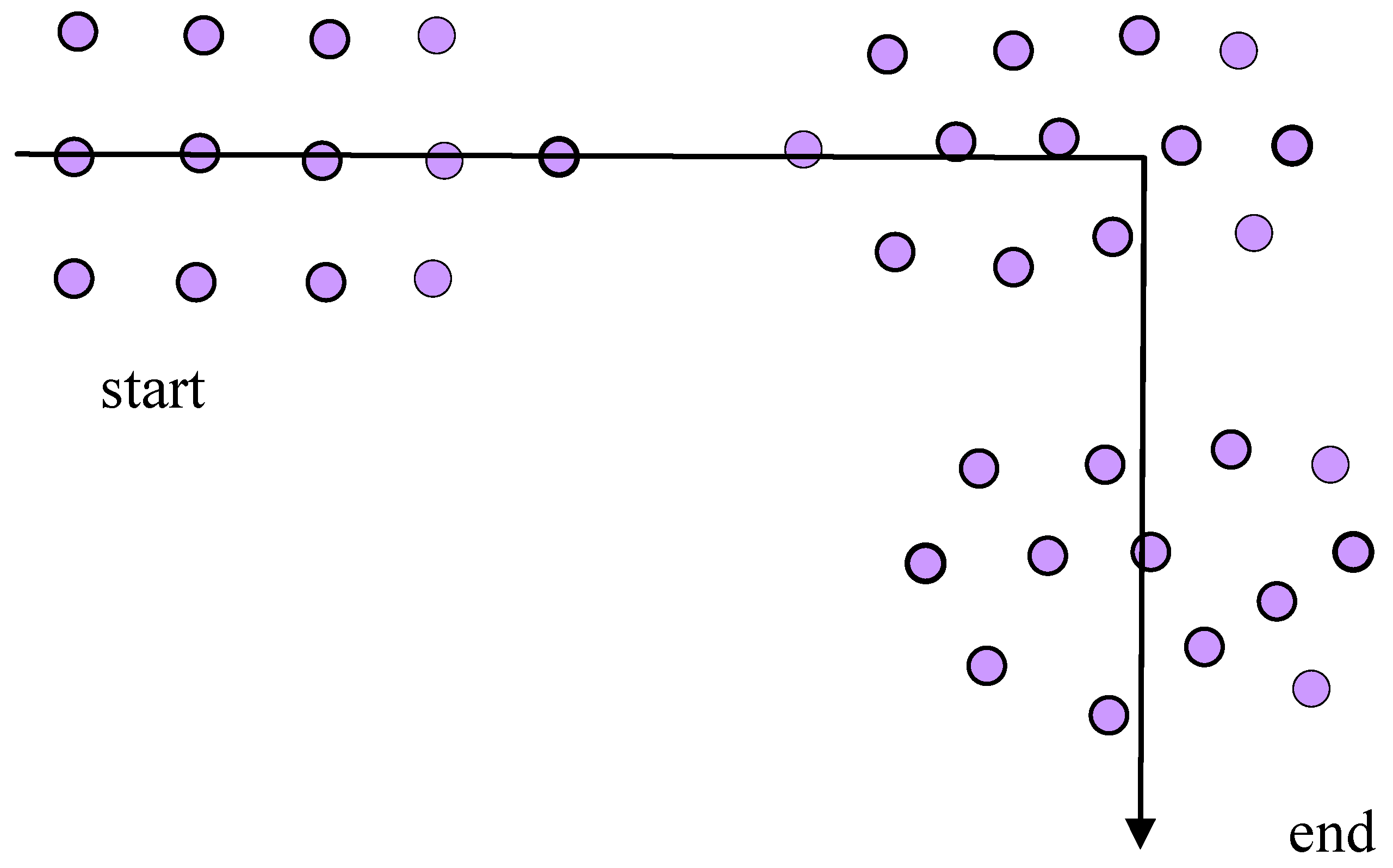
Action 5: The leader was controlled by the operator to pass between obstacles on a rectangular path. Followers/slaves were to follow it and avoid the obstacle.

Results: The operator estimated the turning point in order for the whole swarm to pass the obstacle. The followers tried to follow the robots in front of their column. Due to the non-ideal tracking system algorithms, the robots tried to keep their distance from their predecessor and followers, so they tried to proceed between them. The result was a change in the array’s shape. The area occupied by the robots changed and the robots did not follow the paths of their predecessors. The operator needed to estimate how to control the leader in order to enable the slave robots to follow it and avoid the obstacle. The results are presented in Figure 14, where the sequences of the swarm positions are marked with numbers.

Effects: The operator needed to control the swarm by commanding the leader and observing the whole swarm. The identification of the leader, the first row, and the column members was needed to maintain the array. To allow the followers to avoid the obstacles, additional obstacle detectors were needed. As a result, each robot should be identified and should have an ID marker.

One of the advantages of using a swarm is the expected reliability, because of the number of robots involved.

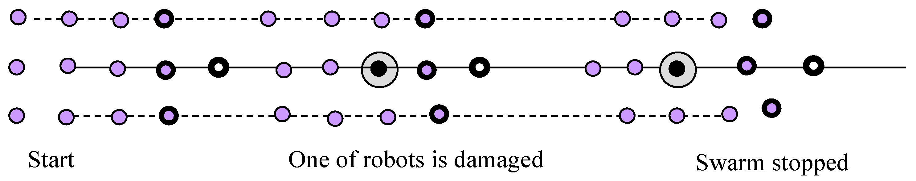
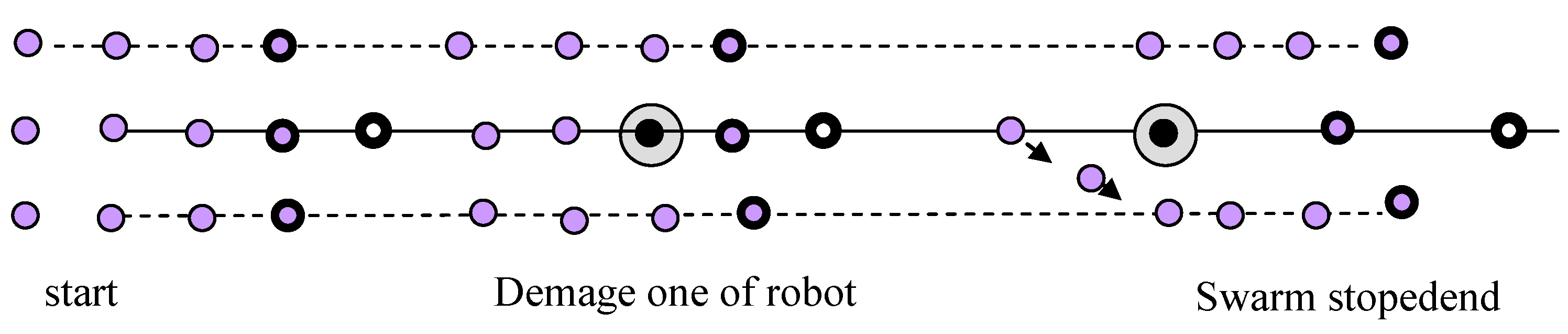
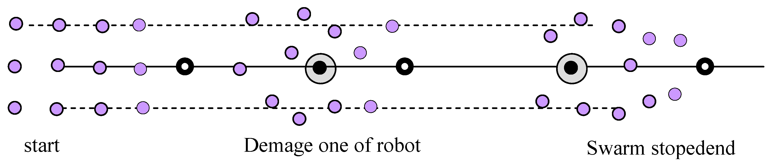
Action 6: The swarm moved straight, but one robot in the swarm failed. The tests were repeated for the leader, first row member, and followers.

Results: The first tests showed that, with control over the distance between the robots, the failure of one robot in the swarm caused the whole swarm to stop. Some changes in the algorithm were introduced in light of the swarm’s behaviour. If a robot’s distance from its predecessor was higher than its distance from its follower, then the stopped robot was “abandoned” by its followers, as shown in Figure 15. Further improvements were made in order for the robots to detect the errors of their the predecessors and join the other column by changing the followed column’s identification. The results are presented in Figure 16.

Effects: Due to their hierarchical structure, the roles of the robots must be defined. If a robot failed, others took up its role. All robots needed to be ready to play all roles in the swarm. Their functions were switched on/off by the remote control system. It was not difficult to send a command changing the role of a chosen robot. It was performed by a protocol structure with successor identification. The biggest problem for the operator was deciding which robot should be the successor, because it was not easy to identify individual robots in the swarm. When we identified robots by column or row number, it was not complicated. After applying changes to the algorithm, individual robots were able to detect errors by a swarm column member and change the column for their followers.

3.2. Nonhierarchical, Random, or Organized Swarm

Due to the results of previous analyses of hierarchical swarm structure, which show that all robots should have the same, quite developed structure, the analysis of basic swarms such as flocks of birds was considered. In flocks of birds or swarms of ants, all members change the direction of movement at the same time [18].

For avoiding problems of the limitation of frequencies, band, and time or operator physical burden, the concept of controlling all robots in a swarm with the same signal simultaneously was tested. According to it, each robot follows the same command respecting the others or the obstacles.

If one common signal is used, there should not be a problem with signal interference or it taking too long to command the swarm.

The pre-adopted robot structure developed for the array was used for analyses. The expected result is the simplification of the robot structure and its acting algorithms.

The main assumptions for the rules of robot action in the swarm are as follows:

• All robots receive control commands and follow them;
• All robots avoid other robots by keeping a defined distance from them;
• Robots detect obstacles individually and avoid them by following the other robots.

As robots affect each other, we can expect that a robot that has not received the command would be “forced” by the others to move the way they do. The structure presented in Figure 17 was used for analyses and simulations.

Action 1: The swarm is moving ahead. The swarm is initially set in an array such as for a structural swarm. Due to the random resistance hampering robots’ movement, the structure changes to a nonregular one.

Results: The swarm keeps roughly to the assumed path. All robots started and stopped at the same time. The result for a swarm set in an array is presented in Figure 18.

Effect: No change is required.

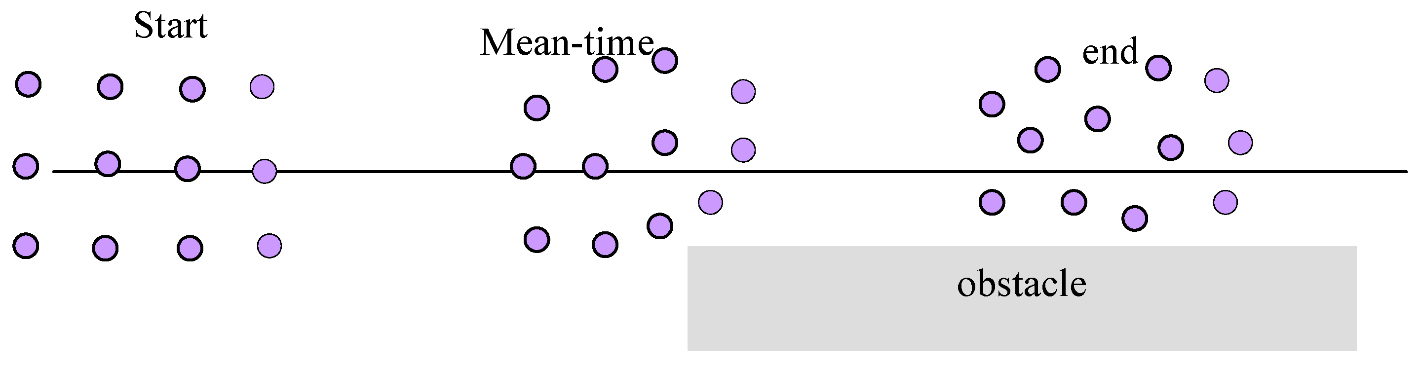
Action 2: The swarm is moving close to the obstacle but the operator does not change the swarm’s trajectory.

Results: The swarm moved around the obstacle as one, stepping away from it.

Effect: No action is required. See Figure 19.

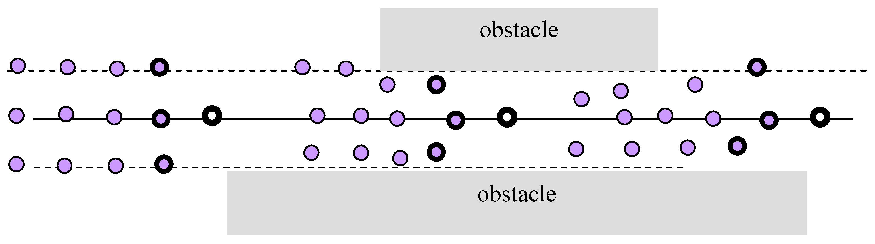
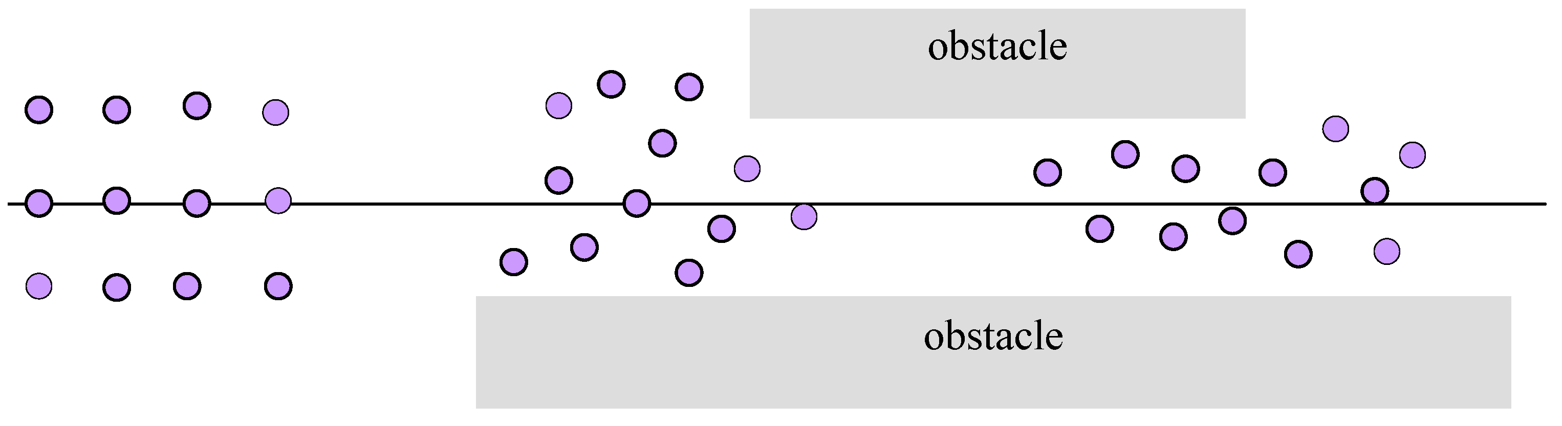
Action 3: The swarm enters between two walls.

Results: The swarm is changing its dimensions: compressing in width and lengthening automatically to keep the appropriate distance between members. After passing through the “corridor,” the structure will be more regular. The result is presented in Figure 20. This is in accordance with our expectations.

Effect. No change is needed.

Action 4: The swarm is turning as a whole, controlled with one signal.

Results: All robots change movement direction at almost the same time. The difference in speed and reaction delay cause the structure to change in a random way. However, the swarm is changing its movement direction as a whole. The simulated result is presented in Figure 21. The result is in accordance with our expectations.

Effect: No improvement is needed.

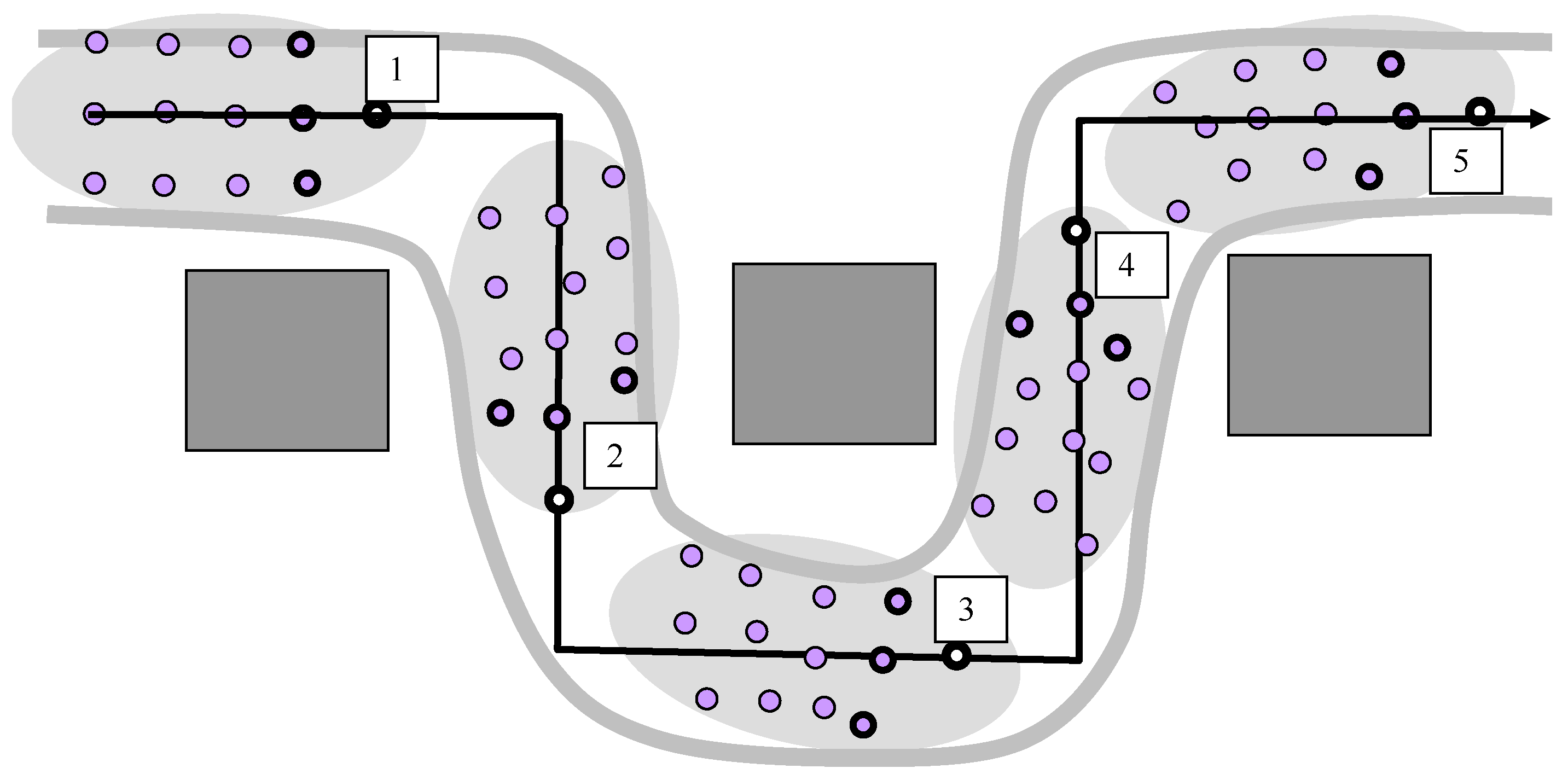
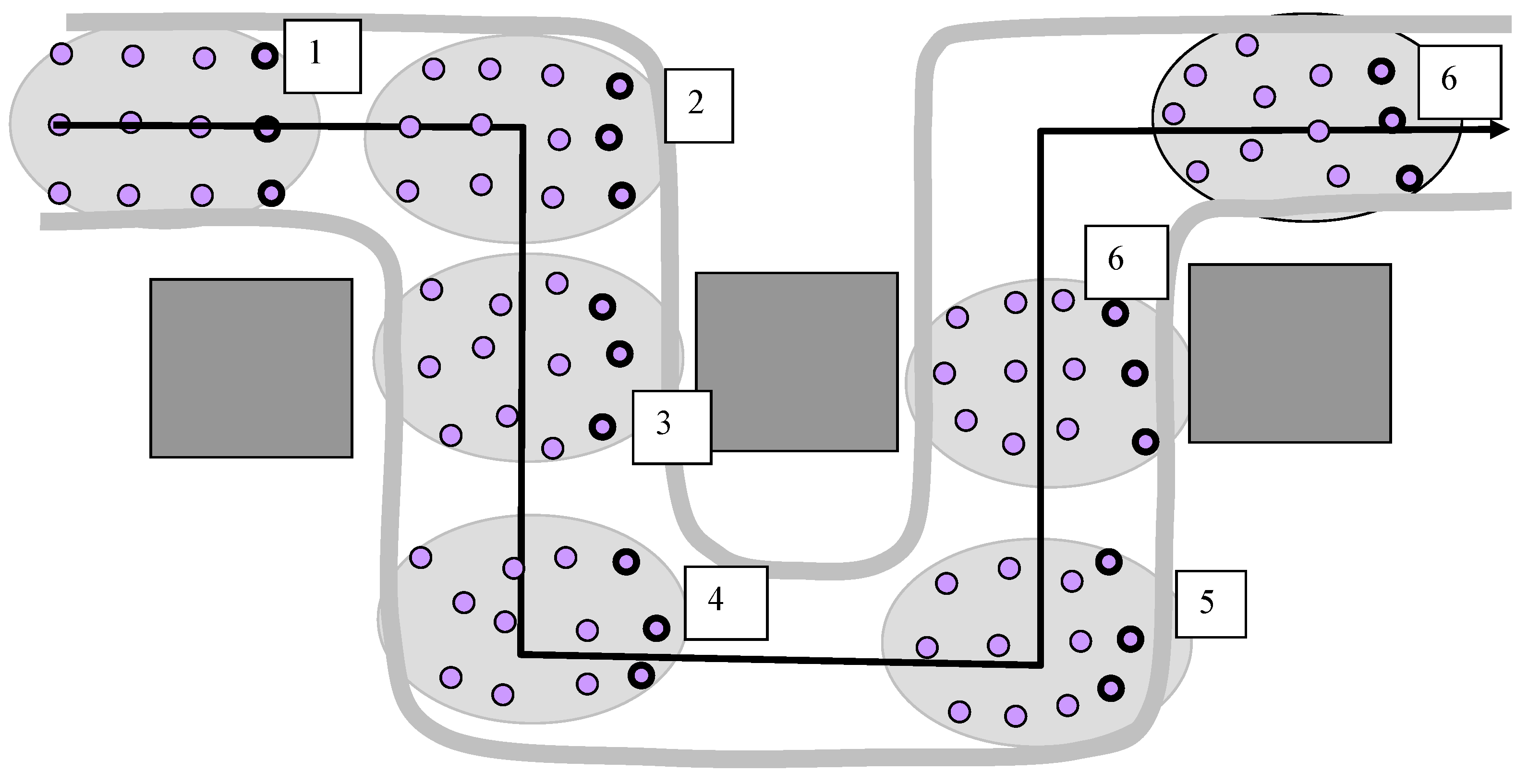
Action 5: The swarm is controlled by an operator to pass between obstacles on a rectangular path. Followers/slaves should follow it and avoid the obstacles.

Results: The operator estimates the place of turning to pass the obstacle as a whole swarm. Robots are trying to keep their distance to neighbours by moving at different and variable speeds. As a result, the swarm changes shape. The area occupied by the robots is changing in some limited range. The operator has to estimate how to control the whole swarm at once. The result is presented in Figure 22, with the sequences of swarm position marked with numbers.

Effects: The operator has to control the swarm by commanding the leader and observing the whole swarm. The identification of the leader, first row, and column members is needed to maintain the array. To avoid the obstacles without breaking the chain of the column, additional obstacle detectors are needed. So, each robot should be identified and have an ID marker.

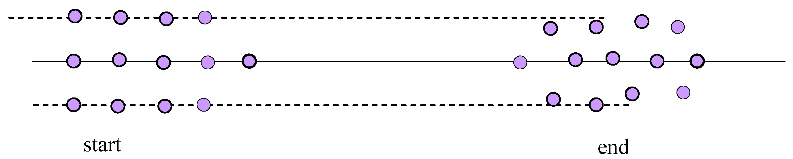
Action 6: The swarm is moving straight, but one robot in the swarm is broken down.

Results: When one robot fails and is not marked as active, other robots treat it as the obstacle, and direct other robots to go around the broken one. The result of the simulation is presented in Figure 23. When the communication system of one robot is broken, the algorithms keeping distance to the others force it to move as a whole swarm.

Effects: A marker of robot state is needed for the identification of the failed robot. If there was a failure of communication, the robots would simply follow the others, keeping their distance from them.

4. Discussion

Initially, the robot swarm based on a soldier array seemed to be easily controlled by controlling the leader. The intelligence of the leader would control the whole swarm. Initially, the structure with a leader was assumed to be the most complicated, but the need for following the leader and avoiding obstacles by followers and the importance of ensuring the swarm fault tolerance meant that the slave robots became more complicated. The leader, which is controlled by the operator, can be the least advanced robot in the swarm.

The analyses and simulation show that a hierarchical structure following the soldier array is complicated and rather expensive to realize with an acceptable level of reliability.

Controlling a swarm by controlling its leader demands from the operator a prediction of all swarm members’ behaviour sequences. The obstacles in the field are avoided by the operator, but individual obstacle detectors are required as well. Keeping the array in a hierarchical structure requires individual robot identification and a definition of their roles and positions in the array. This role should be changeable.

For this reason, the opposite structure of a swarm—nonhierarchical, randomly organized, and applying the simplest rules—was investigated.

The randomly organized swarm met our assumptions and appeared to be more resistant to failure and easier to control than the structural one.

As the random swarm appeared to be resistant to communication breakdowns, it can be assumed that only one robot in the swarm is remotely controlled or programmed. When it is at the centre of a swarm, the whole swarm moves similar to it. We can notice a similar situation in a swarm of bees, where the queen is at the centre but decides the whole swarm’s structure, as presented in Figure 24. When we have more than one robot that is moving in a different direction, the swarm will be broken into a few swarms.

The intelligence and power of a swarm is based on the group-keeping algorithms, which are of the highest priority compared to other criteria.

The majority of swarm members decide about the general direction of movement. Each member tries to keep at a distance from others and avoid obstacles.

In the future, work on the problem of robot domination in a random organized swarm is planned. Knowledge of this will help us to avoid complications during command interpretation error by some robots in a swarm and to gain knowledge on animals’ swarm dividing and joining mechanisms, which could be imitated in robotics.

Two kinds of robot swarm organizations have been analysed. They were modelled with the same robot structure, but for the structural model, ordered speeds were calculated based on distances between robots. In the structural swarm, the distance between robots decided the speed limits, but the speed was ordered by RC.

As the source of swarm intelligence, the high priority of distance-keeping has been pointed out. All results are the effect of it. An unstructured swarm of robots with simultaneous RC seems to be easier to be controlled than a structured one.

The structure and control algorithm of individual robots working in an unstructured swarm seem to be simpler and cheaper to achieve. Those robots do not need to identify their positions in the swarm but only keep their distance from others.

The operator controlling the unstructured swarm as a whole does not need to make predictions of the behaviour and tracking of followers and leads the robots from place to place faster.

A nonhierarchical swarm built with robots controlling its speed and distance to others, an obstacle detector, and an omitting algorithm will create an intelligent swarm that will move faster toward the aim, penetrate the obstacle with minimum energy losses, and be most resistant to individual robot failure.