Investigation of Applicability of Impact Factors to Estimate Solar Irradiance: Comparative Analysis Using Machine Learning Algorithms

Abstract

This study explores investigation of applicability of impact factors to estimate solar irradiance by four machine learning algorithms using climatic elements as comparative analysis: linear regression, support vector machines (SVM), a multi-layer neural network (MLNN), and a long short-term memory (LSTM) neural network. The methods show how actual climate factors impact on solar irradiation, and the possibility of estimating one year local solar irradiance using machine learning methodologies with four different algorithms. This study conducted readily accessible local weather data including temperature, wind velocity and direction, air pressure, the amount of total cloud cover, the amount of middle and low-layer cloud cover, and humidity. The results show that the artificial neural network (ANN) models provided more close information on solar irradiance than the conventional techniques (linear regression and SVM). Between the two ANN models, the LSTM model achieved better performance, improving accuracy by 31.7% compared to the MLNN model. Impact factor analysis also revealed that temperature and the amount of total cloud cover are the dominant factors affecting solar irradiance, and the amount of middle and low-layer cloud cover is also an important factor. The results from this work demonstrate that ANN models, especially ones based on LSTM, can provide accurate information of local solar irradiance using weather data without installing and maintaining on-site solar irradiance sensors.

1. Introduction

Information on solar irradiance and activity is one of the major challenges facing the efficient use of solar power, because solar irradiance has a significant impact on the Earth’s energy system [1]. The use of renewable energy sources has been increasing, such that renewable energy accounted for 18.2% of total global energy consumption in 2016 [2]. Besides the 7.8% of final consumption from traditional biomass, 10.4% of total energy consumption comes from modern renewables consisting of wind, solar, biofuels, ocean power, and others. Moreover, total renewable power capacity reached 2195 GW in 2017 [2]. From the viewpoint of investment, solar energy generation accounted for more than 55% of all newly installed renewable power capacity in 2017, with wind accounting for 29% [2]. Naturally, solar energy generation and building energy consumption have been increasing, especially in China [3,4]. Specifically, building energy consumption has increased with the increase in urbanization throughout the world, and building energy consumption in China is expected to increase drastically by 35% [3]. Hence, effective solar energy generation has become a very important renewable energy source, and the energy provided by increased solar panel installations in buildings can meet this increasing demand for energy, together with traditional fossil energy sources [5,6]. The amount of solar irradiance which passes through walls, the roof, and window materials strongly impacts the thermal energy consumption of buildings. Moreover, electricity energy generated from solar panels is quite reliant on local solar irradiance [7].

The main hypothesis of this study is that this study can estimate long-term solar irradiance using data-driven ANNs methodology based on environmental elements, e.g., temperature, humidity ratio, wind direction, velocity, atmospheric pressure, and amount of cloud cover rate from a meteorological station. Using data processing neural network (NN) structure has an advantage to obtain nonlinear results, which can be obtained through training previous data. Even though the result cannot guarantee the solution of chaotic change of circumstance, the output performance has been proved with relevant performance. Additionally, impact factors are analyzed by four different machine-learning algorithm results, and it has the effect of increasing the accuracy. The impact factor determines how much each input node element value can affect the target result values based on an adjusted value after training with input elements and real target values. In order to forecast future solar irradiance level, the impact factors affected by climatic elements such as local environments or air pollutions can improve, to accurately predict solar irradiance and power generation using photovoltaic (PV) systems [8,9,10,11], and aid the prediction of thermal loads in buildings and can design systems to optimize smart grid networks in urban areas. Moreover, accurate modeling reduces the uncertainty in control algorithms used for battery storage and optimization of electricity usage [8]. However, direct measurement of solar irradiance from irradiance devices has been limited to deduce energy balance of smart grid energy networks and to design the scheduling of power generation. Finally, an accurate model of deduced solar irradiance can also illicit economic benefits in the energy networks and industrial sectors.

There is a rich array of literature describing many methods of predicting solar irradiance with artificial neural networks (ANNs) [12,13,14,15,16,17,18,19,20]. Kamadinata et al. [12] predicted solar irradiance based on sky image data. Cao, J. and Cao, S. developed a method of prediction of solar irradiance using a neural network with sample data by wavelet analysis [21]. Voyant et al., Ahmand et al., and Monjoly et al., presented prediction models based on numerical and hybrid autoregressive moving average (ARMA)/ANN models [13,22]. Watanabe and Nohara studied solar irradiance prediction using one-granule cloud property data [14,23]. Cheng and Yu used predictive modeling based on cloud classification [24]. Sharma et al., showed short term solar irradiance predictions using a mixed wavelet neural network [25]. Dong et al., proposed a model combining satellite image analysis with a hybrid ESSS/ANN model [26]. Further, Mellit et al., evaluated the performance of an adaptive model for forecasting solar irradiance in comparison with a feed-forward neural network model [27]. Some reports have also demonstrated the short- and long-term prediction of solar irradiance with statistical models [28,29,30,31]. Joshi et al., evaluated the accuracy of solar irradiance forecasting using the Australian Bureau of Meteorology’s ACCESS models [32]. Ruiz-Arias and Gueymard used a reference physical radiative transfer model [33]. Murata et al., evaluated solar irradiance modeling uncertainty with the estimation of multiple confidence intervals [34]. Miller et al., presented a short-term forecasting method with satellite model coupling [35]. Ong et al., showed a prediction method using ray-tracing techniques [36]. Aggarwal and Saini presented a solar energy prediction method using linear and non-linear regularization models [37]. Qing and Niu also presented a solar irradiance prediction method using weather forecasts [8]. This study explored deduction strategies for solar irradiance and sensitivity analysis based on actual local climatic parameters using four prediction algorithms: linear regression, support vector machines (SVM), a multi-layer neural network (MLNN), and a long short-term memory (LSTM) network. The comparison is illustrated through impact factor and addressed. We evaluated the performance of these four models using weather data collected over eight years (70,080 hourly data points) as a training set, and one year of data (8760 hourly data points) as a test set. The obtained deduction results were compared with real solar irradiance values. Therefore, this study hypothetically estimates that if weather condition is predictable, solar irradiance is also deduced using ANNs methodologies. To investigate how each environmental element influences the solar irradiance in a city depending on seasonal changes, we also analyzed the performance sensitivity using the four prediction models. From impact factor analysis, we could determine which climate factors strongly influence the solar irradiance, and which factors can be neglected when considering solar irradiance prediction. This study shows the relationship between climate factors and solar irradiance in the four models examined. In this paper, we aim to predict solar irradiance with environmental parameters. Solar irradiance is mainly affected by the angle of incidence and is also influenced by cloud coverage and seasonal changes such as temperature and humidity ratio. This means that machine learning (ML) using an artificial neural network (ANN) structure makes it possible to estimate solar irradiance using satellite data [38,39]. Some previous reports have already discussed the prediction of building energy using environmental elements as inputs [40,41]. Further, it has been reported that the most influential factors for determining electricity usage are temperature and working day information [4]. However, getting information on solar irradiance is limited because the available information is not decisive. This study collected weather data from Seoul, which is the capital and a mega city in South Korea, from the Korea Metrological Administration (KMA) [42] for research purposes. The location of observatory station in Seoul is Songwol-dong, Jongno-gu, Seoul. We used long-term historical hourly weather data for a period of nine years (2008–2016) and the main elements of the weather conditions are temperature, humidity ratio, air pressure, global horizontal irradiance (GHI), cloud data, and wind speed and direction. ANNs training with long term eight-year historical data and solar irradiance data will estimate one-year solar irradiance and the results will be analyzed. Additionally, this study evaluates accuracy of the deducted solar irradiance compared with measured solar irradiance by variable linear and nonlinear data-driven approaches. In the results, this study could define which of the weather elements can significantly impact on the solar irradiance and which elements could be neglected to obtain the information of solar irradiance. Therefore, using the considered weather elements, ANNs can be used to show how each weather parameter or climate changes impact on amount of solar irradiance in the future. Weather is chaotic and in principle not reliably predictable, however there are several works whose solar irradiance prediction based on weather forecasts [8,14]. This study would also point out that due to difficulty in weather forecasting, we consider as many climate elements as possible in the current work. Even when the forecasting is not reliable, the estimation of solar irradiance based on historical climate data could be useful in assessing and planning the solar production, often before the beginning of new construction or installation of solar panels on existing houses and buildings.

This study proposes an estimation strategy to investigate impact factors estimating local solar irradiance based on local weather parameters. We also present a comparison of different methods to deduce solar irradiance including linear regression, SVM, MLNN, and LSTM. This study explores which of the local weather parameters could significantly impact the solar irradiance depending on seasonal changes and local environments if input data are from weather forecasting. The analysis through numerical estimation comprises the following aspects:

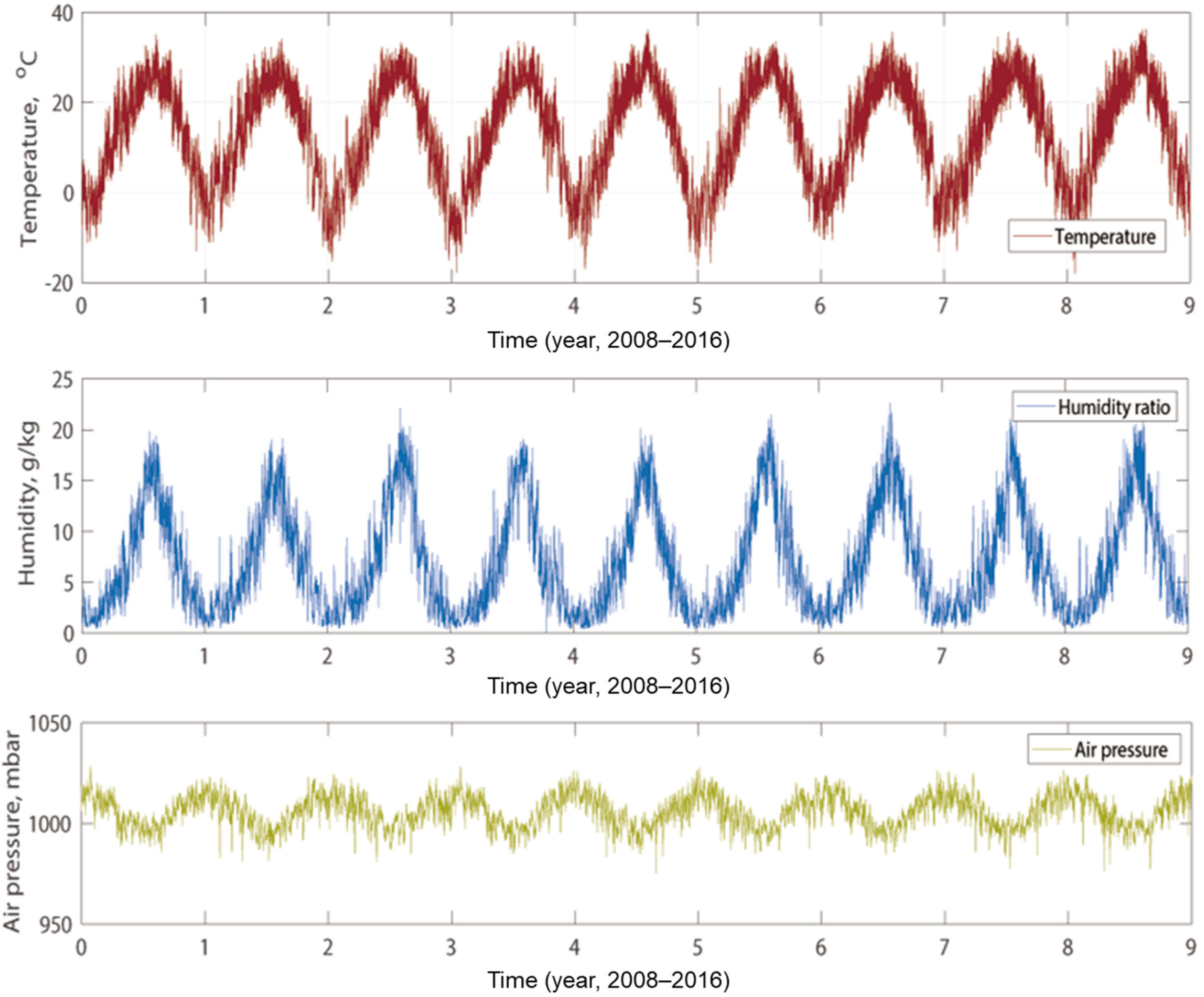
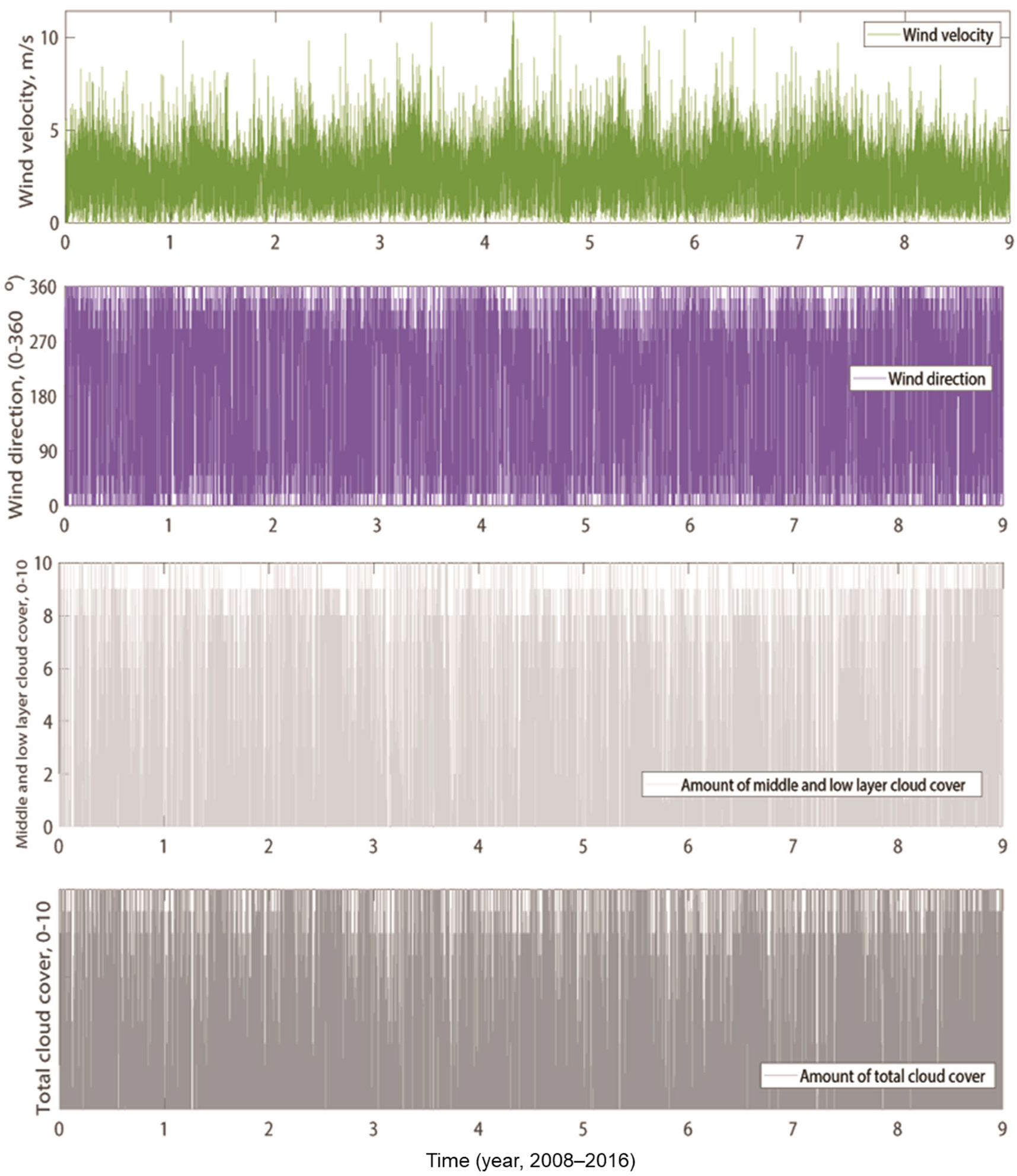
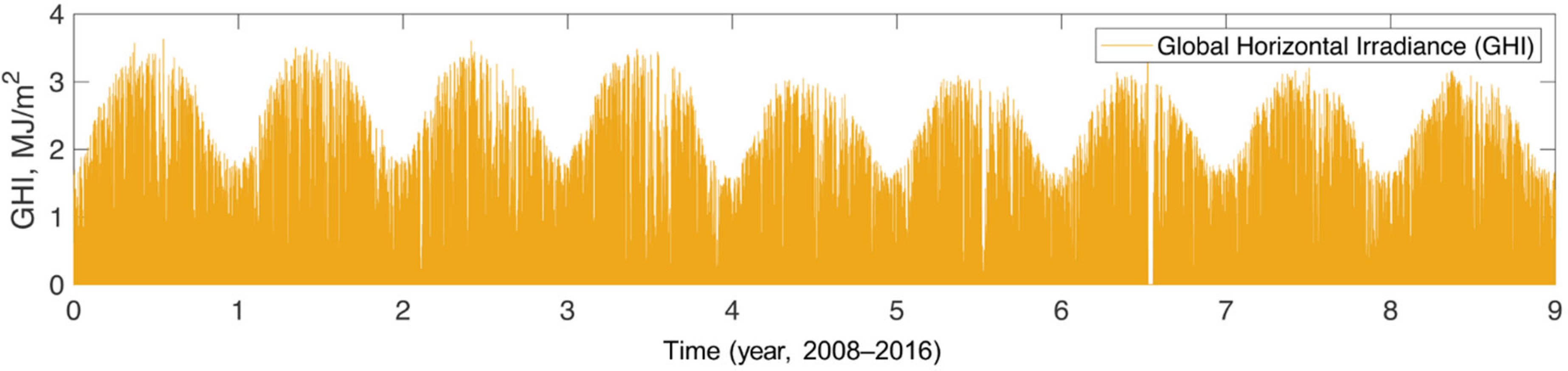
• Collecting hourly nine year local weather data and solar irradiance values
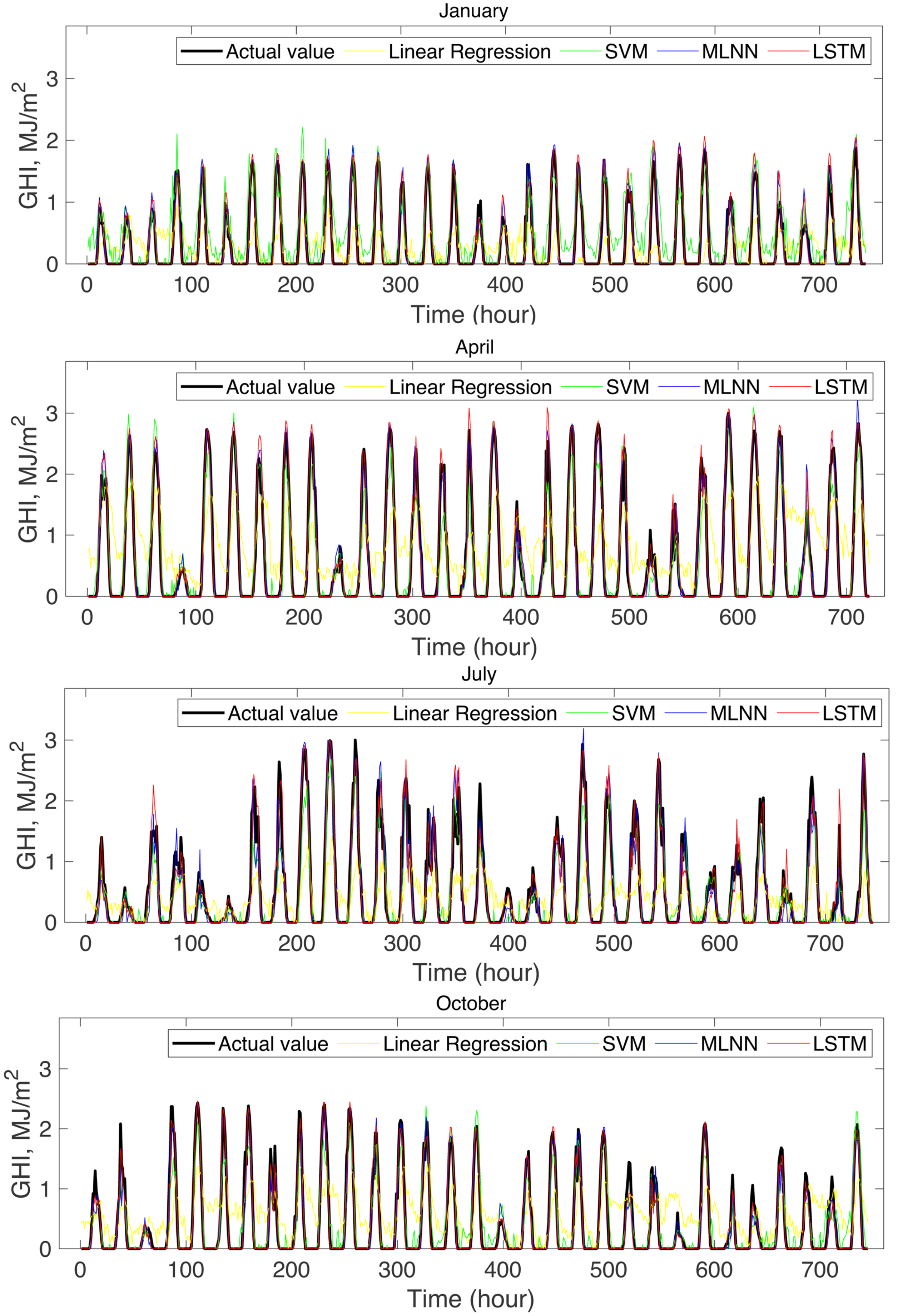
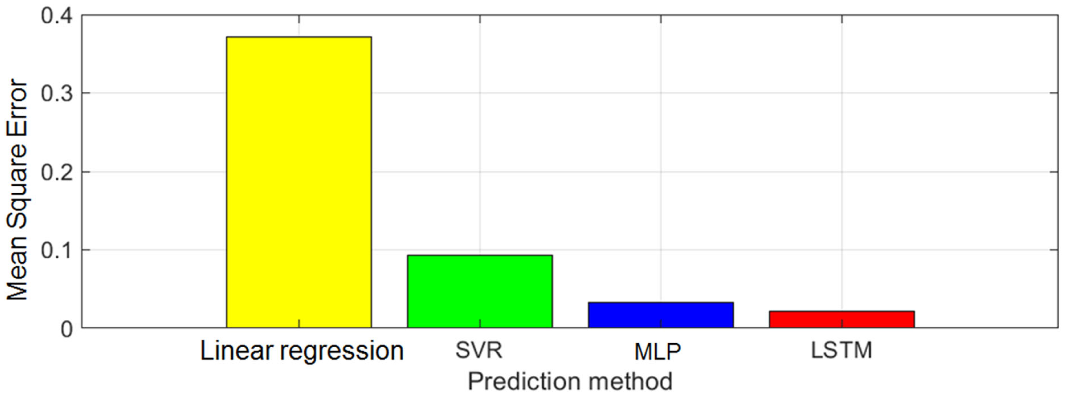
• Estimation of one year solar irradiance using the data with the four different methods: linear regression, SVM, MLNN and LSTM
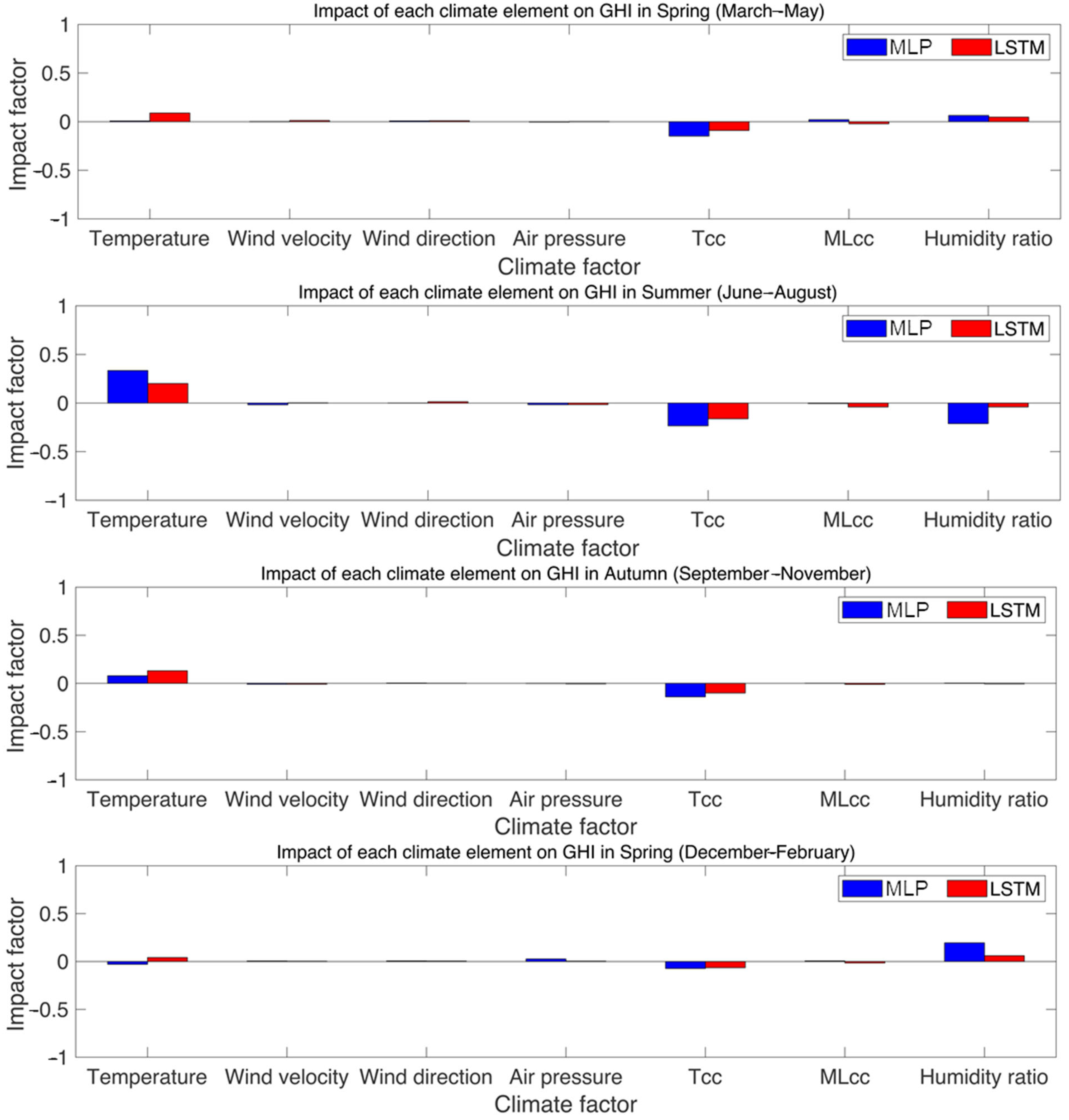
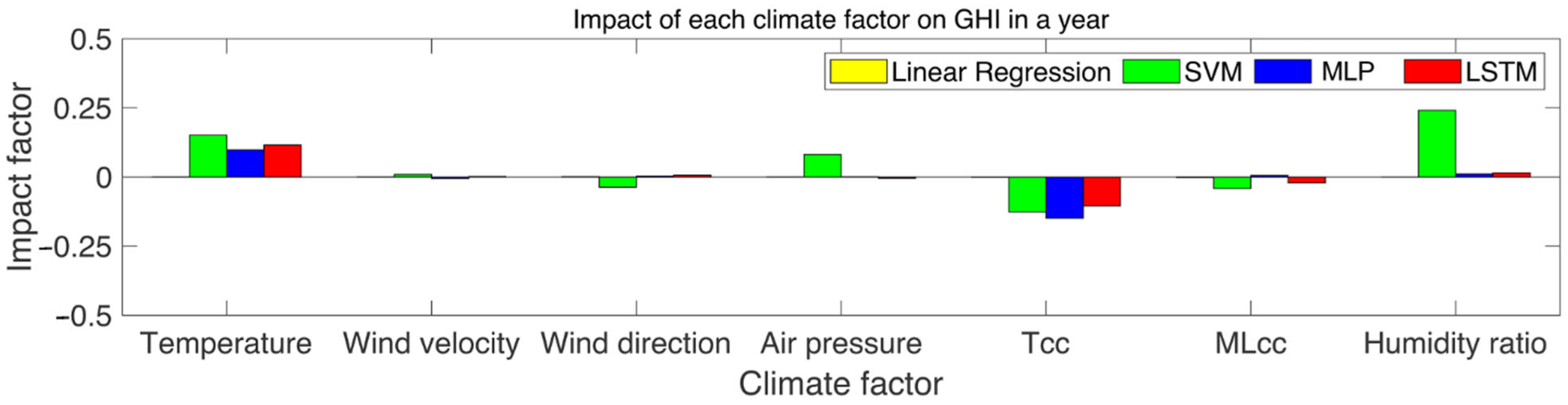
• Analysis of impact factors of each weather parameter
• Comparison of the results and validation of the four estimation methods

2. Methodology

2.1. Linear Regression

Linear regression analysis attempts to model the relationship among variable elements by fitting a linear equation. This approach is based on combinations that can be summarized by a few equations [43]. Linear regression seeks to find a vector such that the function $f$ is a matrix multiplication between $x$ and $\beta$ as follows:

$$f={\beta }_0+x_1 {\beta }_1+x_2 {\beta }_2+x_n {\beta }_n+\mathsf{\epsilon }$$

(1)

where, ${\beta }_0$ is the constant, ${\beta }_1, {\beta }_2\dots , {\beta }_n$ are called the regression coefficients, $x$ denotes the transpose and predictor, $x=\left(x_1,x_2,x_3\dots ,x_n\right)$, and n is the number of variables. The sum of the squares of all the distances between each $x_i$ and ${\beta }_i$ is calculated and the goal is to minimize this sum. $\mathsf{\epsilon }$ is the error therm. This gives a hyper-plane, and the outputs of $f$ are mapped onto this plane.

2.2. Support Vector Machines

While linear regression performs well with a dataset that has a linear relationship between its inputs and outputs [44], we need more advanced methods to address datasets with non-linear relationships. SVM is an effective tool for non-linear regression problems, and it is suitable for predicting solar irradiance and energy consumption [45]. It is a machine learning algorithm [46] and typically used to solve regression problems [47]. SVM is mainly based on statistical learning theory, where the goal is to reduce structural risk by ensuring an upper bound of generation error [46].

SVM uses a kernel $K$ to map the original space onto a higher dimensional space to find a better hyperplane with a certain margin. The margin is defined as the distance between the hyperplane and the closest ${\mathrm{x}}_i$ vectors. SVM not only finds the hyperplane, but also seeks to maximize the margin. Let $\mathsf{\Phi }$ be a map from the original space to the higher dimensional space. Then, a kernel is the dot product of pairs of $\mathsf{\Phi }\left({\mathrm{x}}_i\right)$ and $\mathsf{\Phi }\left({\mathrm{x}}_j\right)$, that is, $K\left({\mathrm{x}}_i, {\mathrm{x}}_j\right)=\mathsf{\Phi }\left({\mathrm{x}}_i\right)·\mathsf{\Phi }\left({\mathrm{x}}_j\right)$. Given the kernel $K$, $f$ is defined by

$$f\left(\mathrm{x}\right)={\displaystyle \sum }_{j=1}^n{\alpha }_{j}k\left({\mathrm{x}}_j, \mathrm{x}\right)+b$$

(2)

for some variables ${\alpha }_i$ and $b$. The goal of SVM is to minimize

$$\lambda {\left|\right|{\displaystyle \sum }_{i=1}^n{\alpha }_i\mathsf{\Phi }\left({\mathrm{x}}_i\right)\left|\right|}^2+\frac{1}{n}{\displaystyle \sum }_{i=1}^{n}L\left(y_i, f\left({\mathrm{x}}_i\right)\right)$$

(3)

where $\lambda$ influences the margin size and $L$ is a loss function between an output of ${\mathrm{x}}_i$ and $y_i$. In this paper, we use a popular kernel which is the radial basis function (RBF) kernel [48], that is,

$$K\left({\mathrm{x}}_i,{\mathrm{x}}_j\right)=\exp \left(-\gamma {\left|\right|{\mathrm{x}}_i-{\mathrm{x}}_j||}^2\right)$$

(4)

for $\gamma >0$. The RBF kernel results in 1 when ${\mathrm{x}}_i={\mathrm{x}}_j$ and approaches zero as ${\mathrm{x}}_j$ moves farther away from ${\mathrm{x}}_i$.

2.3. Artificial Neural Networks (ANNs)

As the amount of accessible data has increased and computers have become faster, more advanced machine learning techniques have emerged. One of the most popular machine learning techniques is deep learning [49], which is the set of methods that use a neural network with multiple layers from the input to the output so that the neural network is able to learn both high- and low-level features. Diverse neural network architectures are used in accordance with learning goals. Feedforward neural networks (MLNNs) are useful for both classification and regression tasks [50,51]. Convolutional neural networks (CNNs) are powerful tools for image classification [52] while recurrent neural networks (RNNs) are well-suited to working with time series data [53]. Other than these architectures, various other types of architectures have also been studied [54,55,56].

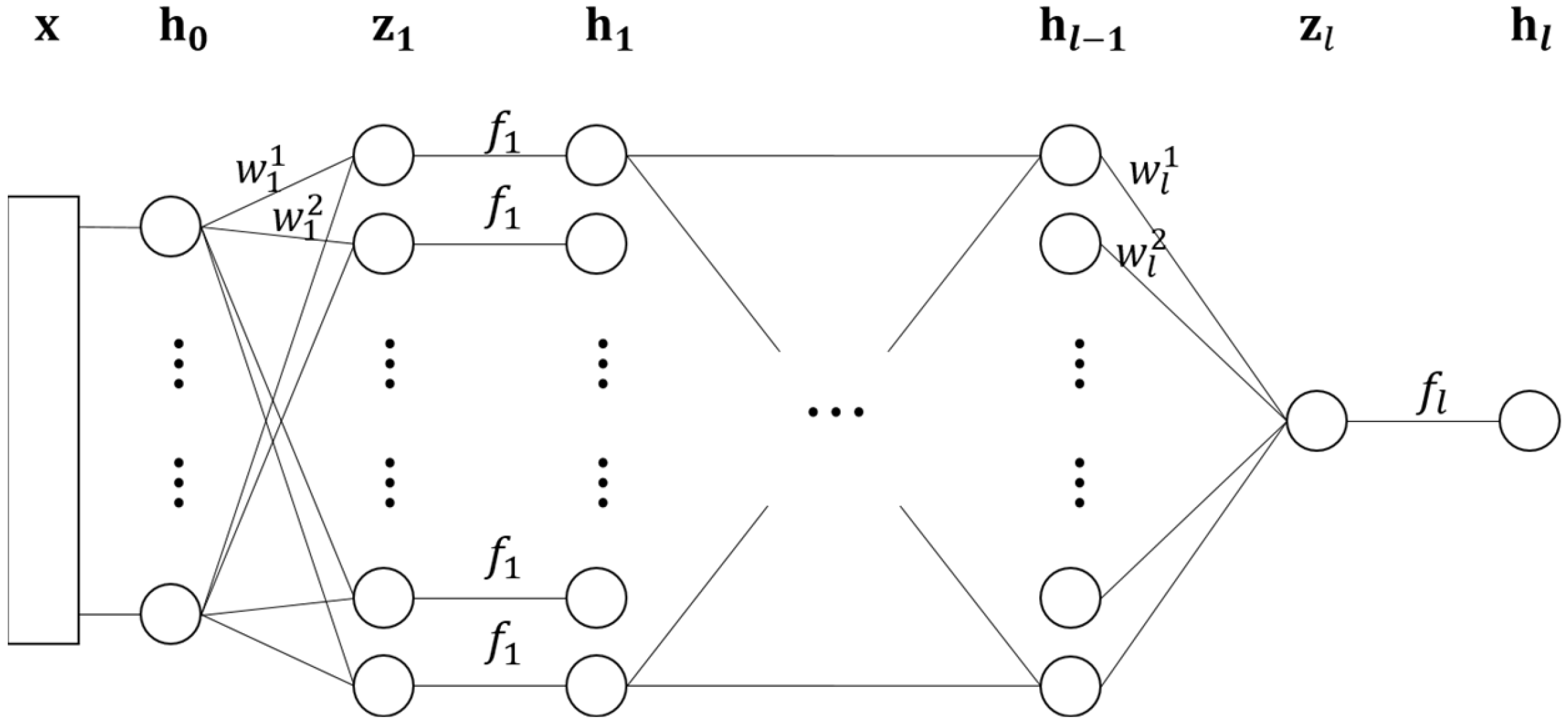
2.3.1. Multi-Layer Neural Network (MLNN)

MLNNs, which are also called feedforward neural networks, have been successfully applied to many research areas for optimization problems because of their improved generalization performance [57,58].

A node in an MLNN is a unit that takes values from the previous layer and calculates a sum of weighted values to produce an output. A layer consists of a number of nodes, and an MLNN has at least three layers: the input layer, one or more hidden layers, and the output layer. During training, an input vector ${\mathrm{x}}_i$ passes through the hidden layers to the output layer. The layer structure is shown in Figure 1.

$${\mathrm{h}}_k=f_k\left({\mathrm{z}}_k\right),$$

(5)

$${\mathrm{z}}_k={\mathrm{w}}_k·{\mathrm{h}}_{k-1},$$

(6)

$${\mathrm{h}}_0={\mathrm{x}}_i,$$

(7)

where $k=1,\cdots ,l$, and ${\mathrm{w}}_k$ and $f_k$ are the weight vector and the activation function in the k-th hidden layer, respectively, such that ${\mathrm{h}}_l$ is the output of the output layer. Then, the loss between the outputs of the MLPs and $y_i$ is calculated and the MLNN proceeds through the backpropagation phase in which it calculates $\frac{\partial L}{\partial w_k^i}$ and $\frac{\partial L}{\partial h_k^i}$, partial derivatives of loss with respect to each weight $w_k^i$ and input $h_k^i$, respectively.

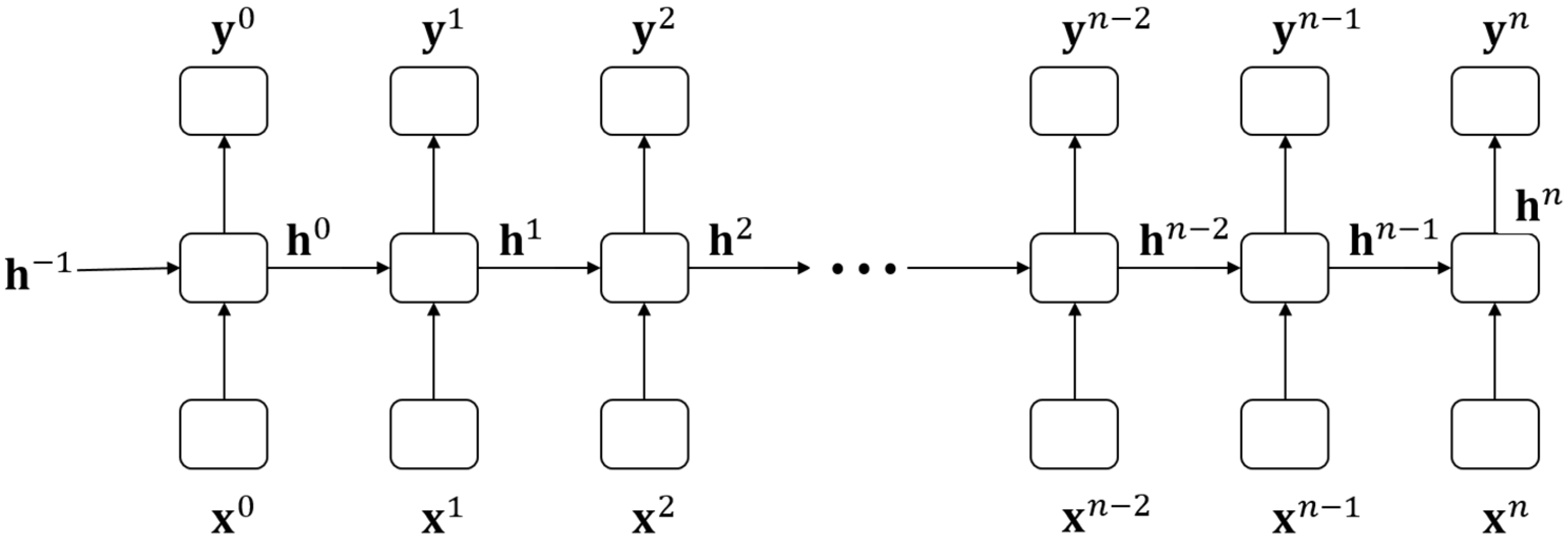
2.3.2. Recurrent Neural Network

Another type of neural network is the recurrent neural network (RNN), which is designed for time series data [53]. These networks have loops so that they consider time dependencies between elements in time-series data. Unlike an MLNN, which takes all elements at once, elements in the time-series data are fed to an RNN sequentially. At each step, an inserted element is concatenated with the output of the previous step, and a new output is computed. This structure is illustrated in Figure 2. Given a time-series data set $\left({\mathrm{x}}^0,{\mathrm{x}}^1, \cdots , {\mathrm{x}}^n\right)$, the equations governing an RNN can be written as follows:

$${\mathrm{y}}^t=g\left({\mathrm{h}}^t\right),$$

(8)

$${\mathrm{h}}^t=f\left({\mathrm{x}}^t,{\mathrm{h}}^{t-1}\right),$$

(9)

where x, y, and h refer to the input, the output, and the hidden state at time step t, respectively.

While RNNs seem to be capable of capturing all dependencies, training an RNN can be unstable due to the problems of exploding gradients or vanishing gradients [49,59]. These problems can be solved using a modification of RNNs, which is called the long short-term memory (LSTM) network [49,59]. An LSTM network is a type of advanced recurrent neural network prediction model, which has achieved remarkable results in many research areas [8,60]. It has a good structure for learning temporal patterns, which makes it useful for various tasks related to time-series analysis [61]. LSTMs have an advantage over conventional modeling using RNNs as they can much more efficiently learn long-term data through their memory cells and gates [62,63]. An LSTM consists of a cell and three kinds of gates. The cell connects the first element to every element in the middle and to the final output. Three gates—forget gate, input gate, and output gate—contribute to updating the cell. The forget gate determines which information the cell forgets. The input gate determines which information the cell updates. Finally, the output gate results in an output at each step based on the input and the cell in the current step.

2.4. Meteorogical Data Collection

The data used in this work was collected from hourly weather data pertaining to Seoul (capital of South Korea), collected over nine years (from 2008 to 2016) by the Korea Metrological Administration. The main elements of the weather conditions are temperature, humidity ratio, global horizontal irradiance (GHI), which is the total amount of shortwave radiation received by a surface horizontal to the ground including direct normal irradiance and diffused horizontal irradiance, cloud data (the amount of total cloud cover, the amount of middle and low-layer cloud cover), air pressure, and wind velocity and direction. Plots of each weather parameter for nine years are shown in Figure 3 and Figure 4.

Figure 3, Figure 4 and Figure 5 present historical climatic factors for nine years: temperature (°C), humidity ratio (g/kg), air pressure (mbar), wind velocity (m/s), wind direction (0–360°), amount of total cloud cover (0–10), amount of middle and low-layer cover (0–10), and global horizontal irradiance (GHI, MJ/m²). Over nine years, 78,840 hourly measurements were collected. As shown in Figure 3, temperature, humidity, and air pressure values had shown periodic patterns regularly with time series analysis every year, and these have similar patterns with solar irradiance variations in Figure 5. However, wind speed, direction, middle layer cloud cover rate and total cloud cover rate have shown a non-periodic pattern. In the training process, ANNs combine periodic and non-periodic pattern parameters. With good structure for learning temporal patterns, it makes it useful for various tasks related to time-series analysis. Therefore, this estimated that ANNs could have more advantages compared with conventional linear or non-linear modeling as they can much more efficiently learn long-term time series data [60,61,62,63].

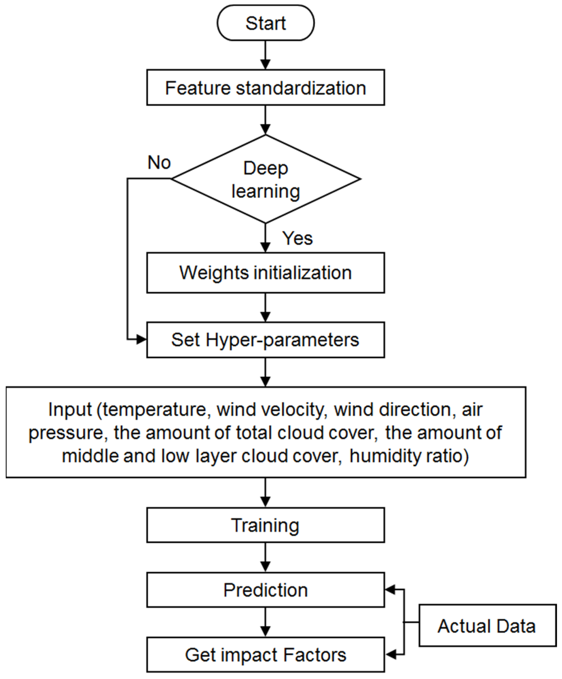
2.5. Training and Estimation

Features are normalized to have zero mean and unit variance and then each hour of data is set as an input $\mathrm{x}$ such that $\mathrm{x}=\left(x_1,x_2\cdots , x_7\right)$ and solar irradiance is set as the output $y$. For an RNN designed for time-series data, the times-series data are constructed as follows:

$$\mathrm{xs}=\left(x_1{}^T, {\mathrm{x}}_2{}^T,\cdots , {\mathrm{x}}_s{}^T\right).$$

(10)

where $s$ is the number of consecutive hours for an input and T is time step index.

We used the weather data for eight years (from 2008 to 2015) as a training set and predicted the solar irradiance value in 2016 as a test set.

To evaluate the accuracy of the simulation results, this study used calibration standards: the mean square error (MSE), widely accepted by ASHRAE Guideline 14-2002 [64]. The corresponding equation is as follows:

$${[\frac{1}{n}{{\displaystyle \sum }}_{i=1}^n{\left(y_i-{\overline{\mathrm{y}}}_i\right)}^2]}^{1/2}$$

(11)

where n is the number of data points, $y_{i }$ is the actual value, and ${\overline{\mathrm{y}}}_i$ is the predicted value.

The network training process is shown in Figure 6.

Generally, in machine learning, SVM, MLNN, and LSTM models require a hyper-parameter whose value is set before the training process can begin. For SVM, we chose a gamma value of 0.1 before learning process. For MLNN, the network used in this study was composed of an input layer, 64 nodes for hidden layer 1, 32 nodes for hidden layer 2, and an output layer. The learning rate was 0.005 and training was conducted for 200 epochs. For the LSTM, we used the same number of layers as the MLNN, and the same learning rate of 0.0005.

To determine the correlations among the weather parameters that impact solar irradiance, we used impact factors, where the magnitude of each value represents the impact and positive or negative values illustrate the direction of the impact. The impact factor evaluation method calculates the impact of each input node element based on an adjusted value after training with input elements and real solar irradiance values. The process used to calculate the impact factor is as follows. After training and testing with all-weather parameters, the test node values are varied between −10% and +10% with an interval of 1% of their original values, to form new testing samples. In order to determine the number of hidden layer nodes, the formula suggested following Equation (12) [40,65]:

$$p<\sqrt{n+m}+a$$

(12)

where p is in the range of numbers, n is the input number, m is the output node number, and a is a positive integer that is less than 10 [40,65].

Subsequently, the new adjusted testing nodes are simulated and compared with the values obtained without adjusting the nodes. Then, each algorithm is used to fit 21 points to a linear functional, and then the gradient of the linear functional is obtained. The gradient is used as the impact of the feature because the gradient describes a linear relation between two variables. The impact values of the features for each machine learning algorithm are illustrated by Equation (13).

$$\underset{\mathsf{\Gamma }}{\min }{\displaystyle \sum }_{i=1}^k{\left(q_i-f\left(p_i,\mathsf{\Gamma }\right)\right)}^2$$

(13)

where min denotes minimizing, q_i and p_i are input values which include 21 data points, and $\mathsf{\Gamma }$ is a set of coefficients.

3. Illustrative Simulation and Analysis

In this study, we used four methods—i.e., linear regression, SVM, MLNN, and LSTM—to deduct local solar irradiance (GHI, MJ/m²). The models were trained using 70,090 hourly data points collected over eight years, consisting of temperature (°C), humidity ratio (g/kg), air pressure (mbar), wind velocity (m/s), wind direction (0–360°), amount of total cloud cover (0–10), amount of middle and low-layer cover (0–10) and were tested using 8760 hourly data points collected over one year. This study explores the accuracy of each model algorithm, and also evaluates how each weather parameter significantly impacts the local solar irradiance. We can estimate long-term solar irradiance without actual radiance sensors based on local weather data and variations. This study used four estimation methods, with weather parameters as the input data and solar irradiance as the output. Based on eight years of training data and one year of testing data, the solar irradiance values were estimated and evaluated by comparison with real values. The performances of the four models were also evaluated based on accuracy and error rate. The results of one-year (January–December) hourly prediction outputs compared with real values are shown in Figure 7. In general, compared to the linear regression and SVM methods, the two ANN models, MLNN and LSTM, exhibited significantly better performance and higher accuracy in deducing solar irradiance. The LSTM model especially showed higher accuracy than the other models. Figure 7 shows that the output of the two ANN models agreed well with the real data; however, the GHI values estimated by linear regression and SVM are even higher than zero during the nighttime. These two algorithms had overshot the estimation values at nighttime. Therefore, these two methods are not suitable for estimating solar irradiance because of their high error rates. Compared with other algorithms, LSTM had relatively overestimated the predicted values in daytime, however, it had good accuracy and the overestimating impact is small.

The mean relative error and mean square error (MSE) results for each model are shown in Figure 8. The MSE results for the linear regression and SVM models were 0.3718 and 0.0932, respectively, and these models showed low accuracy and high error rates compared to those of the two ANN methods. The MLNN and LSTM models achieved MSE values of 0.0324 and 0.0221, respectively. The estimation MSE using LSTM showed a 31.7% increase in accuracy compared to MLNN. Thus, the two ANN models showed higher performance with good accuracy and stability when estimating local solar irradiance. Based on the results, the LSTM showed the best estimation performance out of the four models even though it had regularly overestimated in daytime. The ANN models showed significantly better estimation performance because having multiple layers between the input and output nodes allowed them to learn to activation functions and network configuration parameters to determine the best value and to minimize the error rate.

Figure 9 presents how much each weather parameter impacts on the local solar irradiance, as determined using four prediction algorithms. Temperature and amount of total cloud cover (Tcc) significantly dominate the local solar irradiance because temperature variations represent seasonal changes, and the total cloud cover can directly affect how much solar irradiance can reach the ground surface. However, the linear regression method did not clearly show the impact factor of each parameter. The results obtained using MLNN and LSTM models indicated that four main parameters mainly affect the actual solar irradiance: temperature, amount of total cloud cover, amount of middle and low-layer cloud cover (MLcc), and the humidity ratio. Moreover, other parameters, including air pressure, wind velocity, and wind direction, could be neglected when considering the main environmental influences for estimating solar irradiance.

Figure 10 and

Table 1. Impact factors of input climate elements determined by MLNN and LSTM models in four seasons.

Impact Factor	Temperature	Wind Speed	Wind Direction	Air Pressure	Tcc	MLcc	Humidity Raito
MLNN
Spring	0.0065	0.0010	0.007	−0.003	−0.14	0.02	0.064
Summer	0.33	−0.017	0.00008	−0.0167	−0.234	−0.004	−0.2116
Fall	0.078	−0.0084	0.0035	−0.0006	−0.1367	0.0011	0.00222
Winter	−0.029	0.0045	0.0054	0.026	−0.073	0.0059	0.1948
LSTM
Spring	0.08877	0.012	0.0092	0.00128	−0.090	−0.0213	0.0467
Summer	0.201	0.0023	0.0136	−0.0158	−0.1622	−0.0399	−0.0403
Fall	0.1303	−0.0084	0.00082	−0.00432	−0.097	−0.00957	−0.0040
Winter	0.04	0.0023	0.0040	0.0035	−0.064	−0.0149	0.0602

present how much each climate factor impacts upon the local solar irradiance depending on the season, as determined using two ANN algorithms (MLNN and LSTM). Amount of total cloud cover (Tcc) mainly dominated local solar irradiance. Usually amount of Tcc includes amount of middle and low-layer cloud cover (MLcc) as well, therefore, MLcc is not an independent element and the element information, amount of Tcc could be enough to deduct local solar irradiance. For example, if there is same amount of Tcc but only changed amount of MLcc, the impact is relatively small, because amount of Tcc mainly dominates the local solar irradiance.

Both temperature and amount of Tcc significantly dominate local solar irradiance in the summer season. Temperature and total cloud cover have relatively less impact on the GHI in other seasons. Changes in the humidity ratio impact the solar irradiance, because it also represents seasonal changes. However, during the summer season, the humidity ratio influences the solar irradiance inversely. It is estimated that a high humidity ratio in the summer season is highly related to the amount of total cloud cover and precipitation, because Seoul is located in a hot and humid climate; hence, it experiences heavy rains in the summer season. Other climate factors (such as wind velocity and direction, and air pressure) can be neglected when estimating solar irradiance, because their impact factors are relatively small compared to the major impact sources (temperature, total cloud cover, middle and low-layer cover, and humidity ratio). The major context of this research is the application of ANNs to solar irradiance estimation based on weather parameters which could prove several advantages, e.g., ability to work with insufficient data/ knowledge and higher performance in a broad range of applications over classical techniques like linear regression and principal component analysis (PSA).

The results presented suggest that local solar irradiance in urban or rural areas could be estimable by artificial neural networks based only on weather reports without the need for actual solar irradiance sensors. However, this study is limited, and more factors should be explored via further research. Solar irradiance can also be affected by variable factors such as geomagnetic storm activity with sunspot numbers increased, ozone, aerosols, and pollutants. Future studies should consider additional environmental factors to increase the accuracy of prediction results. Additionally, more regular training with recently updated weather data can efficiently response from future climatic changes unprecedently. Future studies should consider additional environmental factors to increase the accuracy of prediction results with unprecedent climatic data.

4. Discussions

In this research, the methods with linear regression, SVM, MLNN, and LSTM have been applied to deduct local solar irradiance. Weather information prediction is not easy and hard to get precise information. Even such a difficulty happened, it needs irradiance information to energy scheduling. Hence, the artificial intelligence approach is considered by training precious data such as temperature (°C), humidity ratio (g/kg), air pressure (mbar), wind velocity (m/s), and wind direction (0–360°) over eight years. Additionally, cloud cover, middle and low-layer cover were also tested with over one year of data. As a result we estimated long-term solar irradiance, which can be obtained without actual radiance sensors. From the results, MLNN and LSTM show better performance and higher accuracy. As mentioned before, LSTM model and LSTM were not always illustrated to be superior to other methods from an accuracy and impact point of view. From the MSE results, two ANN models showed good performance due to reliable information by NN training. From the impact point of view, this was how much each weather parameter impacted upon the local solar irradiance. Temperature and cloud cover (Tcc) significantly dominated. Then, the results with MLNN and LSTM models showed four main parameters affecting the actual solar irradiance. Additionally, it was shown in Figure 10 and Table 1 that the total cloud cover (Tcc) affects solar irradiance mostly. As a result, temperature and amount of Tcc significantly dominate local solar irradiance in the summer season. However, it is a reverse situation during the summer season because the humidity affects in reverse the solar irradiance. Specifically, the high humidity ratio in the summer is highly related to the total cloud cover and precipitation in Seoul, Korea, because of the climate. To be simplicity; data availability and small impact, wind velocity and direction, and air pressure could be neglected.

The obtained results suggest the estimation of local solar irradiance by artificial neural networks based on weather reports. It helps to plan energy generation scheduling, but it still needs to improve from the limited information. Specially, more variable factors such as geomagnetic storm activity, ozone, aerosols, and pollutants affect solar irradiance; hence, future studies should consider additional environmental factors to increase the accuracy of prediction results.

5. Conclusions

In this study, we explored investigation of applicability of impact factors to estimate solar irradiance using climatic elements including temperature, humidity ratio, the amount of total cloud cover, the amount of middle and low-layer cloud cover, wind velocity and direction, and air pressure. The strategies were based on four machine learning algorithms: linear regression, SVM, MLNN, and LSTM. We evaluated the performance of the four models using eight years of weather data as a training set, and one year of data as a test set. The estimation results were then compared with real solar irradiance values. The results showed that the ANN models provided more accurate estimations of solar irradiance than conventional techniques (such as linear regression and SVM). Among the two ANN models, LSTM provided better performance, improving estimation accuracy by 31.7% compared to MLNN. To investigate the effect of each climate factor on the solar irradiance in a city, we also carried out impact factor analysis with the four estimation models. The results of the impact factor analysis revealed that temperature and the amount of total cloud cover are the dominant factors affecting the solar irradiance, and the amount of middle and low-layer cloud cover is also an important factor. The results from this work demonstrate that ANN models, especially those based on LSTM that consider time correlations in the data, can accurately estimate local solar irradiance using weather data without installing and maintaining on-site solar irradiance sensors. Hence, they can provide a cost-effective method of accurately estimating solar power generation, thermal heat gains, and thermal energy consumption rates in buildings and urban and rural areas. In future works, a study could define the differences of weather conditions between a meteorological station and a local place using ANNs methodologies, and then we could know how local surrounding environments such as high-rise buildings and mountains near a building located impact on solar irradiance. Additionally, we could denote how much air pollutants, such as PM 2.5, PM 10, could impact on solar irradiance using ANN methodologies.

References

1. Kirov, B.; Asenovski, S.; Georgieva, K.; Obridko, V.N.; Maris-Muntean, G. Forecasting the sunspot maximum through an analysis of geomagnetic activity. J. Atmos. Sol.-Terr. Phy. 2018, 176, 42–50. [Google Scholar] [CrossRef]
2. Ren21. Renewables 2018 Global Status Report. Available online: http://www.ren21.net/gsr-2018/ (accessed on 1 September 2021).
3. China, N.E.A.I. National Energy Administration in China; 2015 the state Council of RPC, Beijing, China. Available online: http://english.www.gov.cn/ (accessed on 1 September 2021).
4. Kim, K.M.; Cha, J.; Lee, E.; Pham, H.V.; Lee, S.; Theera-Umpon, N. Simplified Neural Network Model Design with Sensitivity Analysis and Electricity Consumption Prediction in a Commercial Building. Energies 2019, 12, 1201. [Google Scholar] [CrossRef] [Green Version]
5. Pacheco-Torres, R.; Heo, Y.; Choudhary, R. Efficient energy modelling of heterogeneous building portfolios. Sustain. Cities Soc. 2016, 27, 49–64. [Google Scholar] [CrossRef]
6. Chemisana, D.; López-Villada, J.; Coronas, A.; Rosell, J.I.; Lodi, C. Building integration of concentrating systems for solar cooling applications. Appl. Eng. 2013, 50, 1472–1479. [Google Scholar] [CrossRef]
7. Lee, H.S. Thermal Design: Heat Sinks, Thermoelectrics, Heat Pipes, Compact Heat Exchangers, ands Solar Cells; Wiley: Hoboken, NJ, USA, 2010. [Google Scholar]
8. Qing, X.; Niu, Y. Hourly day-ahead solar irradiance prediction using weather forecasts by LSTM. Energy 2018, 148, 461–468. [Google Scholar] [CrossRef]
9. Nixon, J.D.; Dey, P.K.; Davies, P.A. Design of a novel solar thermal collector using a multi-criteria decision-making methodology. J. Clean Prod. 2013, 59, 150–159. [Google Scholar] [CrossRef] [Green Version]
10. Torres, J.F.; Troncoso, A.; Koprinska, I.; Wang, Z.; Martínez-Álvarez, F. Big data solar power forecasting based on deep learning and multiple data sources. Expert Syst. 2019, 36, e12394. [Google Scholar] [CrossRef]
11. Wei, C.-C. Evaluation of Photovoltaic Power Generation by Using Deep Learning in Solar Panels Installed in Buildings. Energies 2019, 12, 3564. [Google Scholar] [CrossRef] [Green Version]
12. Kamadinata, J.O.; Ken, T.L.; Suwa, T. Sky image-based solar irradiance prediction methodologies using artificial neural networks. Renew. Energy 2019, 134, 837–845. [Google Scholar] [CrossRef]
13. Ahmad, A.; Anderson, T.N.; Lie, T.T. Hourly global solar irradiation forecasting for New Zealand. Sol. Energy 2015, 122, 1398–1408. [Google Scholar] [CrossRef] [Green Version]
14. Watanabe, T.; Nohara, D. Prediction of time series for several hours of surface solar irradiance using one-granule cloud property data from satellite observations. Sol. Energy 2019, 186, 113–125. [Google Scholar] [CrossRef]
15. Çelik, Ö.; Teke, A.; Yıldırım, H.B. The optimized artificial neural network model with Levenberg–Marquardt algorithm for global solar radiation estimation in Eastern Mediterranean Region of Turkey. J. Clean Prod. 2016, 116, 1–12. [Google Scholar] [CrossRef]
16. Wang, L.; Shi, J. A Comprehensive Application of Machine Learning Techniques for Short-Term Solar Radiation Prediction. Appl. Sci. 2021, 11, 5808. [Google Scholar] [CrossRef]
17. Herrera, V.M.V.; Soon, W.; Legates, D.R. Does Machine Learning reconstruct missing sunspots and forecast a new solar minimum? Adv. Space Res. 2021, 68, 1485–1501. [Google Scholar] [CrossRef]
18. Ruiz-Arias, J.A.; Gueymard, C.A.; Santos-Alamillos, F.J.; Quesada-Ruiz, S.; Pozo-Vázquez, D. Bias induced by the AOD representation time scale in long-term solar radiation calculations. Part 2: Impact on long-term solar irradiance predictions. Sol. Energy 2016, 135, 625–632. [Google Scholar] [CrossRef]
19. Ruiz-Arias, J.A.; Gueymard, C.A.; Santos-Alamillos, F.J.; Pozo-Vázquez, D. Worldwide impact of aerosol’s time scale on the predicted long-term concentrating solar power potential. Sci. Rep. 2016, 6, 30546. [Google Scholar] [CrossRef] [Green Version]
20. Malik, H.; Garg, S. Long-Term Solar Irradiance Forecast Using Artificial Neural Network: Application for Performance Prediction of Indian Cities. In Applications of Artificial Intelligence Techniques in Engineering; Springer: Singapore, 2019; pp. 285–293. [Google Scholar]
21. Cao, J.C.; Cao, S.H. Study of forecasting solar irradiance using neural networks with preprocessing sample data by wavelet analysis. Energy 2006, 31, 3435–3445. [Google Scholar] [CrossRef]
22. Voyant, C.; Muselli, M.; Paoli, C.; Nivet, M.-L. Numerical weather prediction (NWP) and hybrid ARMA/ANN model to predict global radiation. Energy 2012, 39, 341–355. [Google Scholar] [CrossRef] [Green Version]
23. MP Garniwa, P.; AA Ramadhan, R.; Lee, H.-J. Application of Semi-Empirical Models Based on Satellite Images for Estimating Solar Irradiance in Korea. Appl. Sci. 2021, 11, 3445. [Google Scholar] [CrossRef]
24. Cheng, H.-Y.; Yu, C.-C. Multi-model solar irradiance prediction based on automatic cloud classification. Energy 2015, 91, 579–587. [Google Scholar] [CrossRef]
25. Sharma, V.; Yang, D.; Walsh, W.; Reindl, T. Short term solar irradiance forecasting using a mixed wavelet neural network. Renew. Energy 2016, 90, 481–492. [Google Scholar] [CrossRef]
26. Dong, Z.; Yang, D.; Reindl, T.; Walsh, W.M. Satellite image analysis and a hybrid ESSS/ANN model to forecast solar irradiance in the tropics. Energy Convers. Manag. 2014, 79, 66–73. [Google Scholar] [CrossRef]
27. Mellit, A.; Eleuch, H.; Benghanem, M.; Elaoun, C.; Pavan, A.M. An adaptive model for predicting of global, direct and diffuse hourly solar irradiance. Energy Convers. Manag. 2010, 51, 771–782. [Google Scholar] [CrossRef]
28. Paulescu, M.; Paulescu, E. Short-term forecasting of solar irradiance. Renew. Energy 2019, 143, 985–994. [Google Scholar] [CrossRef]
29. Sun, F.; Gramacy, R.B.; Haaland, B.; Lu, S.; Hwang, Y. Synthesizing simulation and field data of solar irradiance. Stat. Anal. Data Min. ASA Data Sci. J. 2019, 12, 311–324. [Google Scholar] [CrossRef] [Green Version]
30. Hou, M.; Zhang, T.; Weng, F.; Ali, M.; Al-Ansari, N.; Yaseen, M.Z. Global Solar Radiation Prediction Using Hybrid Online Sequential Extreme Learning Machine Model. Energies 2018, 11, 3415. [Google Scholar] [CrossRef] [Green Version]
31. Chang, J.F.; Dong, N.; Ip, W.H.; Yung, K.L. An ensemble learning model based on Bayesian model combination for solar energy prediction. J. Renew. Sustain. Energy 2019, 11, 043702. [Google Scholar] [CrossRef]
32. Joshi, B.; Kay, M.; Copper, J.K.; Sproul, A.B. Evaluation of solar irradiance forecasting skills of the Australian Bureau of Meteorology’s ACCESS models. Sol. Energy 2019, 188, 386–402. [Google Scholar] [CrossRef]
33. Ruiz-Arias, J.A.; Gueymard, C.A. A multi-model benchmarking of direct and global clear-sky solar irradiance predictions at arid sites using a reference physical radiative transfer model. Sol. Energy 2018, 171, 447–465. [Google Scholar] [CrossRef]
34. Murata, A.; Ohtake, H.; Oozeki, T. Modeling of uncertainty of solar irradiance forecasts on numerical weather predictions with the estimation of multiple confidence intervals. Renew. energy 2018, 117, 193–201. [Google Scholar] [CrossRef]
35. Miller, S.D.; Rogers, M.A.; Haynes, J.M.; Sengupta, M.; Heidinger, A.K. Short-term solar irradiance forecasting via satellite/model coupling. Sol. Energy 2018, 168, 102–117. [Google Scholar] [CrossRef]
36. Ong, R.H.; King, A.J.C.; Caley, M.J.; Mullins, B.J. Prediction of solar irradiance using ray-tracing techniques for coral macro- and micro-habitats. Mar. Environ. Res. 2018, 141, 75–87. [Google Scholar] [CrossRef]
37. Aggarwal, S.K.; Saini, L.M. Solar energy prediction using linear and non-linear regularization models: A study on AMS (American Meteorological Society) 2013–14 Solar Energy Prediction Contest. Energy 2014, 78, 247–256. [Google Scholar] [CrossRef]
38. Svozil, D.; Kvasnicka, V.; Pospichal, J. Introduction to multi-layer feed-forward neural networks. Chemom. Intell. Lab. Syst. 1997, 39, 43–62. [Google Scholar] [CrossRef]
39. Tetlow, R.M.; van Dronkelaar, C.; Beaman, C.P.; Elmualim, A.A.; Couling, K. Identifying behavioural predictors of small power electricity consumption in office buildings. Build Environ. 2015, 92, 75–85. [Google Scholar] [CrossRef]
40. Ye, Z.; Kim, M.K. Predicting electricity consumption in a building using an optimized back-propagation and Levenberg–Marquardt back-propagation neural network: Case study of a shopping mall in China. Sustain. Cities Soc. 2018, 42, 176–183. [Google Scholar] [CrossRef]
41. Zhu, Y.; Kim, M.K.; Wen, H. Simulation and Analysis of Perturbation and Observation-Based Self-Adaptable Step Size Maximum Power Point Tracking Strategy with Low Power Loss for Photovoltaics. Energies 2018, 12, 92. [Google Scholar] [CrossRef] [Green Version]
42. Administration, K.M. Weather data, Korea Metrological Administration. Available online: www.kma.go.kr (accessed on 1 September 2019).
43. Pino-Mejías, R.; Pérez-Fargallo, A.; Rubio-Bellido, C.; Pulido-Arcas, J.A. Artificial neural networks and linear regression prediction models for social housing allocation: Fuel Poverty Potential Risk Index. Energy 2018, 164, 627–641. [Google Scholar] [CrossRef]
44. Yan, X.; Su, X.G. Linear Regression Analysis: Theory and Computing; World Sceintific: Singarpore, Singarpore, 2009. [Google Scholar] [CrossRef]
45. Zhong, H.; Wang, J.; Jia, H.; Mu, Y.; Lv, S. Vector field-based support vector regression for building energy consumption prediction. Appl. Energy 2019, 242, 403–414. [Google Scholar] [CrossRef]
46. Meenal, R.; Selvakumar, A.I. Assessment of SVM, empirical and ANN based solar radiation prediction models with most influencing input parameters. Renew. Energy 2018, 121, 324–343. [Google Scholar] [CrossRef]
47. Duan, H.; Huang, Y.; Mehra, R.K.; Song, P.; Ma, F. Study on influencing factors of prediction accuracy of support vector machine (SVM) model for NOx emission of a hydrogen enriched compressed natural gas engine. Fuel 2018, 234, 954–964. [Google Scholar] [CrossRef]
48. Buhmann, M.D. Radial Basis Functions [Electronic Resource]: Theory and Implementations; Cambridge University Press: Cambridge, UK, 2003. [Google Scholar]
49. LeCun, Y.; Bengio, Y.; Hinton, G. Deep learning. Nature 2015, 521, 436–444. [Google Scholar] [CrossRef] [PubMed]
50. Hornik, K.; Stinchcombe, M.; White, H. Multilayer Feedforward Networks Are Universal Approximators. Neural. Netw. 1989, 2, 359–366. [Google Scholar] [CrossRef]
51. White, H. Connectionist Nonparametric Regression—Multilayer Feedforward Networks Can Learn Arbitrary Mappings. Neural. Netw. 1990, 3, 535–549. [Google Scholar] [CrossRef]
52. Krizhevsky, A.; Sutskever, I.; Hinton, G.E. ImageNet Classification with Deep Convolutional Neural Networks. Commun. ACM 2017, 60, 84–90. [Google Scholar] [CrossRef]
53. Graves, A.; Mohamed, A.R.; Hinton, G. Speech Recognition with Deep Recurrent Neural Networks. In Proceedings of the 2013 IEEE International Conference on Acoustics, Speech and Signal Processing, Vancouver, BC, Canada, 26–31 May 2013. [Google Scholar]
54. Kingma, D.P.; Welling, M. Auto-Encoding Variational Bayes. arXiv 2013, arXiv:1312.6114. [Google Scholar]
55. Xian, Y.; Schiele, B.; Akata, Z. Zero-Shot Learning—The Good, the Bad and the Ugly. In Proceedings of the IEEE Conference on Computer Vision and Pattern Recognition, Honolulu, HI, USA, 22–25 July 2017. [Google Scholar]
56. Radford, A.; Metz, L.; Chintala, S. Unsupervised Representation Learning with Deep Convolutional Generative Adversarial Networks. arXiv 2015, arXiv:1511.06434. [Google Scholar]
57. Ban, J.-C.; Chang, C.-H. The learning problem of multi-layer neural networks. Neural. Netw. 2013, 46, 116–123. [Google Scholar] [CrossRef] [PubMed]
58. Kamimura, R. SOM-based information maximization to improve and interpret multi-layered neural networks: From information reduction to information augmentation approach to create new information. Expert. Syst. Appl. 2019, 125, 397–411. [Google Scholar] [CrossRef]
59. Greff, K.; Srivastava, R.K.; Koutník, J.; Steunebrink, B.R.; Schmidhuber, J. LSTM: A Search Space Odyssey. arXiv 2015, arXiv:1503.04069. [Google Scholar] [CrossRef] [Green Version]
60. Yang, B.; Sun, S.; Li, J.; Lin, X.; Tian, Y. Traffic flow prediction using LSTM with feature enhancement. Neurocomputing 2019, 332, 320–327. [Google Scholar] [CrossRef]
61. Baek, Y.; Kim, H.Y. ModAugNet: A new forecasting framework for stock market index value with an overfitting prevention LSTM module and a prediction LSTM module. Expert. Syst. Appl. 2018, 113, 457–480. [Google Scholar] [CrossRef]
62. Göçken, M.; Özçalıcı, M.; Boru, A.; Dosdoğru, A.T. Integrating metaheuristics and Artificial Neural Networks for improved stock price prediction. Expert. Syst. Appl. 2016, 44, 320–331. [Google Scholar] [CrossRef]
63. Yuan, X.; Chen, C.; Jiang, M.; Yuan, Y. Prediction interval of wind power using parameter optimized Beta distribution based LSTM model. Appl. Soft Comput. 2019, 82, 105550. [Google Scholar] [CrossRef]
64. ASHRAE. ASHRAE Guideline 14–2002: Measurement of Energy and Demand Savings; ASHRAE: Atlanta, GA, USA, 2002. [Google Scholar]
65. Amber, K.P.; Aslam, M.W.; Hussain, S.K. Electricity consumption forecasting models for administration buildings of the UK higher education sector. Energy Build 2015, 90, 127–136. [Google Scholar] [CrossRef]
Figure 1. Multi-layer neural network structure.
Applsci 11 08533 g001
Figure 2. Recurrent neural network structure.
Applsci 11 08533 g002
Figure 3. Historical data for 9 years (2008–2016): temperature, humidity ratio, and air pressure.
Applsci 11 08533 g003
Figure 4. Historical data for 9 years (2008–2016): wind velocity, wind direction, amount of middle, low-layer cloud cover (MLcc) and amount of total cloud cover (Tcc).
Applsci 11 08533 g004
Figure 5. Historical data for 9 years (2008–2016): Global Horizontal Irradiance (GHI).
Applsci 11 08533 g005
Figure 6. Training process for artificial neural network.
Applsci 11 08533 g006
Figure 7. Estimation output of four models compared with real values (January–April–July–October).
Applsci 11 08533 g007
Figure 8. Comparison of four modeling error.
Applsci 11 08533 g008
Figure 9. Impact factor of input climate elements determined by four methods.
Applsci 11 08533 g009
Figure 10. Impact factors of input climate elements determined by ANN models in four seasons.
Applsci 11 08533 g010