Abstract
In this work, an artificial neural network (ANN) model was efficiently developed to predict the pyrolysis of mixed plastics, including pure polystyrene (PS), polypropylene (PP), low-density polyethylene (LDPE), and high-density polyethylene (HDPE), at a heating rate of 60 K/min using thermogravimetric analysis (TGA) data. The data of seventeen experimental tests of polymer mixtures with different compositions were used. A feed-forward back-propagation model, with 15 and 10 neurons in two hidden layers and TANSIG-TANSIG transfer functions, was constructed to predict the weight left percent during the pyrolysis of the mixed polymer samples. The model input variables include the composition of each polymer (PS, PP, LDPE, and HDPE), and temperature. The results showed an excellent agreement between the experimental and the predicted weight left percent values, where the correlation coefficient (R) is greater than 0.9999. In addition, to validate the proposed model, a highly efficient performance was found when the proposed model was simulated using new input data. Furthermore, a sensitivity analysis was performed using Pearson correlation to find the uncertainties associated with the relationship between the output and the input parameters. Temperature was found to be the most sensitive input parameter.
1. Introduction
The global generation rate of municipal solid waste (MSW) has reached 2.01 Bt/year and it is expected to reach 2.59 Bt/year by 2030 [1]. In Saudi Arabia, 5.2% of the MSW is plastic waste [2]; 15.3 Mt/year of MSW was generated in 2014 and the rate is expected to reach 30 Mt/year by 2033 [3]. Due to the current challenges of plastic recycling, most of the plastic waste is either incinerated or disposed of in landfills, and thus produced harmful products and emissions causing critical environmental issues [4]. The pyrolysis of plastic waste has been considered as a promising alternative treatment option where oil and gas products, with high caloric values, can be used as fuel for some engines.
Constantinescu et al. [5] investigated the products (oil and/or gas) of the pyrolysis of low-density polyethylene (LDPE), high-density polyethylene (HDPE), polypropylene (PP), and polystyrene (PS). The effect of catalysts on the pyrolysis products was studied using lignite and zeolite catalysts. It was reported that the caloric values of the produced oil ranged between 40.17 and 45.35 MJ/kg, and thus it was recommended as an alternative fuel for diesel engines. In addition, the produced oil had a lower sulfur content that was found to be below the acceptable limit. Furthermore, the produced gas was rich in hydrocarbons and has caloric values ranging between 73.42 and 121.18 MJ/kg.
In addition, Constantinescu et al. [6] explored the types of oil and gas produced from the pyrolysis of PP, polyethylene (HDPE and LDPE), and PS. Two mesoporous silica materials (MCM-41 and SBA-15) were used. A positive effect of the catalyst on the caloric values of the produced oil and gas was reported. Also, it was claimed that the produced oil and gas are much cheaper than those available on the market.
In Saudi Arabia, plastic wastes mainly comprise LDPE, HDPE, PS, polyvinyl chloride (PVC), and PP [7].
Due to its powerful performance to predict efficiently different experimental data, artificial neural network (ANN) modeling has attracted the attention of many researchers to be used for a variety of engineering applications. For example, ANN models can be used to predict the thermogravimetric analysis (TGA) data of the materials’ thermal decomposition (pyrolysis).
In 2004, Conesa et al. [8] developed, for the first time, an ANN model to predict the kinetic parameters of the pyrolysis of some materials using TGA-experimental data at different heating rates. Bezerra et al. [9] predicted the TGA data of the pyrolysis of carbon-reinforced fiber composites and carbon fibers using ANN. Two input parameters (temperature and heating rate) and an output layer (mass retained) were used. The optimum ANN topology was reported as 2-21-21-1. Burgaz et al. [10] used ANN to predict the thermal stability and crystallinity of the mixture of polyethylene oxide and clay using experimental data obtained by differential scanning calorimetry (DSC), dynamic mechanical analysis (DMA), and TGA. For TGA experiments, an ANN model, with a feed-forward back-propagation, Levenberg–Marquardt (LM) algorithm, and TANSIG–LOGSIG–purelin transfer function, for the first and second hidden layers, was structured. Temperature and clay weight percent were the input parameters to predict weight loss percent. Excellent performance, with a regression coefficient of 0.99994, was reported.
Yıldız et al. [11] developed an ANN model to predict the weight loss percent during the thermal decomposition of some blends with different compositions using non-isothermal TGA data covering a wide temperature range (298–1273 K). Three input parameters, namely temperature, blend ratio, and heating rate, were used as the input variables. Good performance of the proposed model was reported.
Çepelioĝullar et al. [12] investigated the weight loss of a refuse-derived fuel during its pyrolysis process by developing an ANN model using TGA data. Two input parameters (heating rate, and temperature) were used. Transfer functions and the number of neurons in each hidden layer were optimized to obtain the best structure of the proposed model. The best-reported topology includes seven to eight neurons with TANSIG-LOGSIG-purelin transfer functions.
Charde et al. [13] developed an ANN model to predict some of the kinetic parameters of the thermal decomposition of the mixture of polycarbonate and CaCO3 using TGA experimental data. Three input parameters (temperature, conversion, and time) were used. Two statistical parameters, namely mean squared error and regression coefficient, were used to identify the best architecture of the proposed ANN model. Chen et al. [14] investigated the thermodynamic and kinetic characteristics of the combustion of some blends at different CO2/O2 ratios. In addition, an ANN model, with three input parameters (heating rate, temperature, and CO2/O2 ratio), was developed to predict the mass loss percent using TGA data. In 2018, Naqvi et al. [15] developed an ANN model using TGA data to predict the thermal decomposition of a sewage sludge that has a high ash contact. Good performance of the proposed ANN model was reported.
Bong et al. [16] studied the effect of microalgae ash catalysts on the pyrolysis of a mixture of a peanut shell and pure microalgae at different heating rates (10–100 K/min). Like the rest of the previous researchers, an ANN model, with heating rate and temperature as input variables, was developed to predict the weight loss percent of the mixture during its thermal decomposition using TGA data.
Dubdub and Al-Yaari [17,18] and Al-Yaari and Dubdub [19] performed comprehensive investigations aiming to obtain the kinetic parameters of the pyrolysis of LDPE, catalytic pyrolysis of HDPE, and the co-pyrolysis of different polymer mixtures including PS, PP, LDPE, and HDPE. In addition, ANN modeling was attempted to predict the weight loss percent using TGA experimental data [17,18]. Excellent agreement between the experimental and predicted results was reported.
Sathiya Prabhakaran et al. [20] investigated the combustion of pet coke under an oxygen atmosphere at three different heating rates (10, 50, and 75 K/min) from 308 to 1173 K. An ANN model with LM algorithm was developed to predict the mass loss percent as a function of temperature and heating rate. A single-layer perception model (SLP) 2-6-1 and a multi-layer perception model between 2-14-6-1 and 2-14-7-6-1, with 11 different models, were tested. Three statistical parameters, namely coefficient of variation (R2), sum of deviation square (SS), and mean residual (MR), were used to evaluate the proposed models. The best architecture model was reported as NN7-MLP2, 2-14-7-6-1.
Liew et al. [21] investigated the catalytic co-pyrolysis of corn cob and high-density polyethylene (HDPE) at a wide range of heating rates (10–200 K/min) and temperatures (323–1173 K). One of the main objectives of that work was to develop an ANN model to predict the co-pyrolysis behavior and determine the thermogravimetric curves as a function of temperature, heating rate, and mixing ratio.
Although extensive work has been performed to develop ANN models to predict the thermal decomposition data of pure polymers/materials, there is insufficient work targeting mixed plastic wastes. Therefore, this work aims to develop an efficient ANN model to predict the pyrolysis data of mixtures of four different polymers (PS, PP, LDPE, and HDPE) using experimental data published earlier [17]. In addition, sensitivity analysis using Pearson correlation was performed.
2. Materials and Methods
2.1. Experiments
The four different polymer samples (PS, PP, LDPE, and HDPE) were characterized using proximate and ultimate analyses. Details of both analyses are reported elsewhere [17] and analysis data are presented in Table 1. The experimental matrix of all TGA tests, with different mixture compositions, at a 60 K/min heating rate is presented in Table 2.

Table 1.
Proximate and ultimate analysis of different waste plastics.
Table 2.
Experimental matrix.
2.2. Topology of ANNs
Process modeling requires the complete identification of the significant process variables whose values must be obtained experimentally. However, the model development and the experimental estimation of the variables are challenging in many conditions and become very difficult as the process complexity (non-linearity) increases. Thus, ANN modeling has attracted researchers’ attention as a powerful promising alternative option, but it needs computational effort [22]. However, after the identification of the process influenced parameters, experimental data must be representative, sufficient, and covering the variation margin of each parameter [23].
Typically, an ANN topology includes input, hidden, and output layers of neurons, and each layer must have a weight, a bias, and an output vector [24]. In addition, each layer has a transfer function connecting input and output layers.
Usually, the experimental (raw) data are divided into three subsets: a training set to establish the network learning and adjust the parameter weight as per the error function; a validation set to check the performance of the network; and, finally, a test set to test the generalization of the network [24].
To find the best structure of an ANN, it is required to optimize the number of hidden layers, the number of neurons in each layer, and the transfer function. The number of neurons in each hidden layer is a crucial parameter having a significant influence on the performance of the developed ANN model. Therefore, underfitting (too few neurons) and overfitting (too many neurons) should be avoided, and the optimum number of neurons must be obtained [25,26]. For this purpose, the prediction performance of different ANN architectures was checked.
Some statistical parameters, including correlation coefficient (R), root mean square error (RMSE), mean absolute error (MAE), and mean bias error (MBE) were used to evaluate the proposed ANN model. Their equations are presented below [27,28].
where Yexp is the experimental value of the weight left percent, Yest is the ANN-estimated value of the weight left percent;; and is the average value of weight left percent.
In addition, sensitivity analysis was performed using Pearson correlation (Equation (5)) to investigate the uncertainties associated with relationships between input and output parameters.
where X and Y are input and output parameters, respectively, and and are their mean values, respectively.
3. Results and Discussion
3.1. Raw Data
Using the thermogravimetric analyzer (TGA7), produced by PerkinElmer (Waltham, MA, USA), the TGA data were obtained, and the kinetic analysis of the experimental results is described elsewhere [17]. In this work, the obtained TGA data were used to develop the targeted ANN model.
3.2. Performance of the Developed ANN Model
The highly efficient ANN model was developed to predict the thermal behavior of mixed polymers. Specifically, the weight left percent of the tested mixtures, as a function of temperature, heating rate, and mixture composition, was targeted to be predicted by the proposed ANN model.
By the “nntool function” in MATLAB 2021a, developed by MathWorks Inc., Natick, Massachusetts, USA, the experimental datasets used for the training stage were divided randomly into three sets: 70% for training, 15% for validation, and 15% for testing.
In this investigation, an ANN model with a feed-forward and back-propagation scheme was developed using 534 datasets. Then, the developed model was validated using an extra 34 datasets during the simulation stage. The datasets’ distribution between training and simulation stages is presented in Table 3.
Table 3.
Datasets distribution between the training and simulation stages for all tests.
The best-developed model has two hidden layers with 15 and 10 neurons, respectively (i.e., 5-15-10-1). In addition, the TANSIG-TANSIG transfer functions and the linear transfer function (Pureline) for the output layer were recommended to be used. Moreover, among different algorithms that were checked, the Levenberg–Marquardt (LM) algorithm was recommended for this network [29]. The network topology of the proposed model is presented in Figure 1.
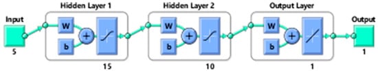
Figure 1.
Topology of the best ANN network (5-15-10-1).
Figure 2 presents the performance of the proposed ANN model (5-15-10-1) for all stages. The results indicate an excellent agreement between the experimental (X-axis) and the predicted (Y-axis) values of the output parameter as indicated by the R-value.
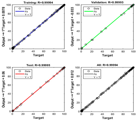
Figure 2.
Regression of training, validation, and test plots.
The prediction performance of the 5-15-10-1 model was evaluated by the values of R, MAE, RMSE, and MBE. Although a high R-value is preferable, the values of other statistical measurements (MAE, RMSE, and MBE) should be low for a high-efficient ANN model. As presented in Table 4, a high R-value (R ≥ 0.9999), and low values of MAE, RMSE, and MBE were obtained. These values imply the high-efficient performance of the developed model to predict the output parameter.
Table 4.
Statistical parameters of the (5-15-10-1) ANN model.
Table 5 shows the parameters of the developed ANN model, and the “goal” was the mean square error (MSE), which was set to zero. Figure 3 shows the performance plot through the training, validation, and test errors when predicting the experimental values. The testing was stopped when validation error increased consecutively for six epochs. In this case, an optimum value of MSE (MSE = 0.13715) was obtained. This value is very small and additionally proves the good prediction performance of the developed model [30,31,32].
Table 5.
Parameters of the developed ANN model.
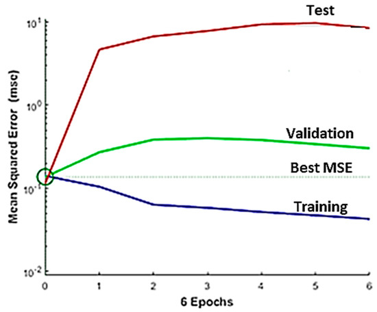
Figure 3.
Optimum mean squared error.
Furthermore, Figure 4 shows the error histogram for the training dataset, which is drawn across the zero error. The error lies only in a narrow range (−1.609 to 1.784), which also indicates the good performance of the proposed ANN model.
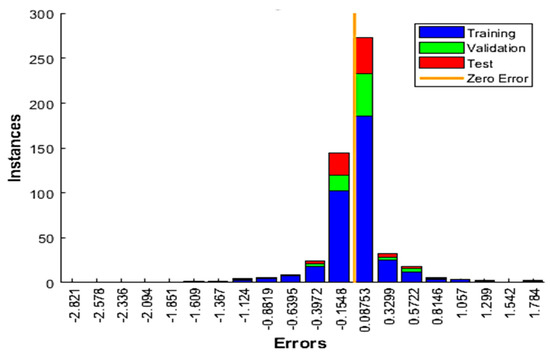
Figure 4.
Error histogram of training data for the (5-15-10-1) network.
To validate the proposed model, it was then checked with 34 new datasets. Table 6 presents the targeted values of the weight left percent of the plastic mixtures during the simulation stage using the new datasets.
Table 6.
ANN-targeted weight left values using the new input datasets for the simulation step.
Figure 5, where the predicted and experimental values are in a full agreement, proves also the high-efficient performance of the ANN model using the new simulated datasets. In addition, as presented in Table 7, the R-value was very high (>0.996) and very low values of MAE, RMSE, and MBE were obtained. Thus, it can be easily concluded that the developed ANN model efficiently predicted the TGA experimental data. An error histogram was created for the simulation data and is shown in Figure 6. As shown in the figure, the error lies also in a small range (−4.334 to 7.605).
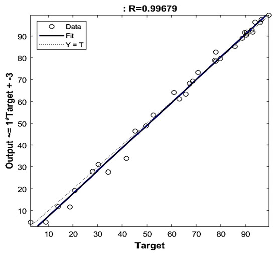
Figure 5.
Regression of the simulated datasets for the (5-15-10-1) ANN model.
Table 7.
Statistical parameters of the (5-15-10-1) model for the simulated data.
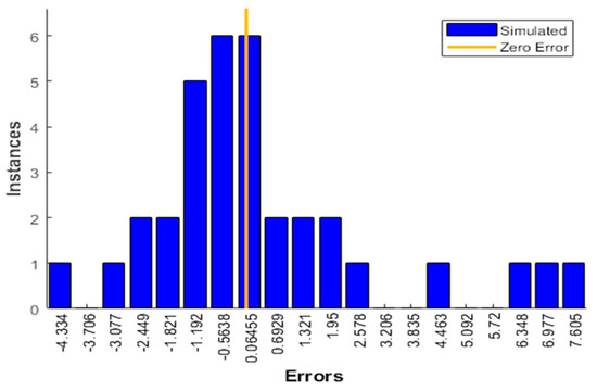
Figure 6.
Error histogram of the (5-15-10-1) ANN model for the simulated datasets.
3.3. Sensitivity Analysis
After the validation stage of a developed ANN model, it is necessary to gain an idea about the uncertainties associated with the relationships between the output (weight left percent) and the input parameters. In general, sensitivity analysis aims to check the effect of a small change in an input parameter on the output variable. In this work, sensitivity analysis, which is a statistical tool to qualitatively obtain the relationship between input and output parameters [33,34,35,36,37,38,39], was performed using Pearson correlation (Equation (5)). In addition, the Pearson correlation indicates whether the relationship is positive or negative. For this purpose, 534 data points were used.
The sensitivity analysis index (SAI), bounded by −1 and +1, was obtained using Pearson correlation. While +1 denotes the maximum proportional effect of an input variable on the output parameter, −1 indicates the maximum inverse impact, and 0 signifies the absence of any correlation between the output and the input [40]. Based on the SAI value, the relationship between an input parameter and the output parameter can be classified as follows: negligible (0 ≤ SAI ≤ ±0.2), weak (±0.21 ≤ SAI ≤ ±0.35), moderate (±0.36 ≤ SAI ≤ ±0.67), strong (±0.68 ≤ SAI ≤ ±0.90), and very strong (±0.91 ≤ SAI ≤ ±1.00) [41]. The results of the analysis are presented in Table 8.
Table 8.
Relative importance of the input parameters.
As per the classification mentioned above, the results presented in Table 8 prove a strong negative correlation between temperature and weight left percent of the mixed plastic during its pyrolysis, which makes sense. As temperature increases, pyrolysis will take place, and thus weight left percent will decrease. This finding is aligned with the thermogravimetric curves, presented elsewhere [17], which have an inverted S-shape.
However, since the SAI values of other parameters are close to zero, the correlation between the composition of the mixed plastic and weight left percent is negligible (no clear correlation), and this can be attributed to the size of the pyrolytic samples (10 mg) and the nature of the thermal decomposition of the polymer samples (fast process).
The statistical significance of the input parameters was then checked with a confirmatory data analysis based on the probability or p-values, which were calculated using the “Regression” function available in the “Data Analysis” toolbox in Excel. The p-values provide a qualitative idea about the most significant parameters. A significance level of 5% (i.e., α = 0.05) was considered for the analysis. This means a parameter was considered statistically significant if the corresponding p-value was less than 0.05 [42,43,44,45]. The results of the analysis are summarized in Table 9.
Table 9.
The p-values of the input parameters.
The results presented in Table 8 and Table 9 imply that temperature is the most sensitive parameter, which is in a good agreement with the results reported by Kempel et al. [46]. Temperature is a key parameter that contributes to the energy needed to transform a unit mass of solids to volatiles [47]. Figure 7 presents the variation in the pyrolysis output parameter (weight left percent) with input parameters. Although the temperature has a clear inverted sigmoid function relationship with weight left percent (Figure 7a), other parameters have no clear correlation with the output parameter (Figure 7b–e).
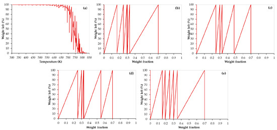
Figure 7.
Effect of input parameters on the output parameter: (a) temperature, (b) PP weight fraction, (c) PS weight fraction, (d) HDPE weight fraction, and (e) LDPE weight fraction.
In addition, as per the above-mentioned criteria, the fractions of mixed plastics are the least sensitive parameters compared with temperature. However, a local sensitivity analysis is highly recommended to confirm this finding.
4. Conclusions
Globally, plastic waste has become one of the major sources causing environmental issues. Although plastic waste has different types and compositions, it mainly includes polypropylene (PP), polystyrene (PS), high-density polyethylene (HDPE), low-density polyethylene (LDPE), polyvinyl chloride (PVC), and polyethylene terephthalate (PET). Pyrolysis is considered a promising technique to treat plastic waste to produce oil and chemicals.
In this work, a high-efficient ANN model was developed to predict the thermal decomposition of mixed polymers including PS, PP, LDPE, and HDPE. The weight left percent of mixed polymers during the pyrolysis process was targeted to be predicted as a function of temperature and a mixture composition using TGA data at 60 K/min.
The best model architecture, with a regression coefficient value of R > 0.9999, has two hidden layers with 15 and 10 neurons, respectively. In addition, the Levenberg–Marquardt training function and tangent sigmoid transfer function were recommended as well.
Then, the proposed network topology was simulated with new input datasets and the predicted results were in excellent agreement with the experimental values with a very high value of R (0.99678) and very low MAE, RMSE, and MBE values. This proves that the ANN model can efficiently predict the pyrolysis TGA data of mixed plastics and can be used for other complex pyrolysis processes.
Moreover, sensitivity analysis using Pearson correlation was performed to identify the uncertainties associated with the relationships between the output (weight left percent) and the input parameters. The results showed that temperature is the most sensitive input parameter.
To extend this work, it is recommended to investigate the produced oil and gas and their caloric values to maximize the benefit of pyrolysis in seeking alternative fuels. In addition, a local sensitivity analysis can be performed.
Author Contributions
Both authors contributed significantly to the completion of this article, but they had different roles in all aspects. Conceptualization, I.D. and M.A.-Y.; data curation, I.D.; formal analysis, I.D. and M.A.-Y.; funding acquisition, I.D.; investigation, I.D. and M.A.-Y.; methodology, I.D. and M.A.-Y.; project administration, I.D. and M.A.-Y.; software, I.D.; validation, M.A.-Y.; visualization, I.D. and M.A.-Y.; writing—original draft, I.D. and M.A.-Y.; writing—review and editing, M.A.-Y. All authors have read and agreed to the published version of the manuscript.
Funding
This research and the APC were funded by the Deanship of Scientific Research at King Faisal University (Saudi Arabia), Nasher Track 2020 (Grant No. 206052).
Institutional Review Board Statement
Not applicable.
Informed Consent Statement
Not applicable.
Acknowledgments
The authors gratefully thank the Deanship of Scientific Research at King Faisal University (Saudi Arabia) for the financial support under Nasher Track 2020 (Grant No. 206052).
Conflicts of Interest
The authors declare no conflict of interest.
References
- Kaza, S.; Yao, L.; Bhada-Tata, P.; VanWoerden, F. What a Waste 2.0: A Global Snapshot of Solid Waste Management to 2050; The World Bank: Washington, DC, USA, 2018. [Google Scholar] [CrossRef]
- Ouda, O.K.M.; Cekirge, H.M.; Raza, S.A. An assessment of the potential contribution from waste-to-energy facilities to electricity demand in Saudi Arabia. Energy Convers. Manag. 2013, 75, 402–406. [Google Scholar] [CrossRef]
- Nizami, A.S.; Ouda, O.K.M.; Rehan, M.; El-Maghraby, A.M.O.; Gardy, J.; Hassanpour, A.; Kumar, S.; Ismail, I.M.I. The potential of Saudi Arabian natural zeolites in energy recovery technologies. Energy 2016, 108, 162–171. [Google Scholar] [CrossRef]
- Silvarrey, L.S.D.; Phan, A.N. Kinetic study of municipal plastic waste. Int. J. Hydrogen Energy 2016, 41, 16352–16364. [Google Scholar] [CrossRef] [Green Version]
- Constantinescu, M.; Bucura, F.; Ionete1, R.E.; Niculescu, V.C.; Ionete, E.I.; Zaharioiu, A.; Oancea, S.; Miricioiu, M.G. Comparative study on plastic materials as a new source of energy. Mater. Plast. 2019, 56, 41–46. [Google Scholar] [CrossRef]
- Constantinescu, M.; Bucura, F.; Ionete1, R.E.; Ebrasu, D.I.; Sandru, C.; Zaharioiu, A.; Marin, F.; Miricioiu, M.G.; Niculescu, V.C.; Oancea, S.; et al. From plastic to fuel—New challenges. Mater. Plast. 2019, 56, 721–729. [Google Scholar] [CrossRef]
- Jan, M.R.; Shah, J.; Gulab, H. Catalytic conversion of waste high-density polyethylene into useful hydrocarbons. Fuel 2013, 105, 595–602. [Google Scholar] [CrossRef]
- Conesa, J.A.; Caballero, J.A.; Reyes-Labarta, J.A. Artificial neural network for modelling thermal decompositions. J. Anal. Appl. Pyrolysis 2004, 71, 343–352. [Google Scholar] [CrossRef]
- Bezerra, E.M.; Bento, M.S.; Rocco, J.A.F.F.; Iha, K.; Lourenço, V.L.; Pardini, L.C. Artificial neural network (ANN) prediction of kinetic parameters of (CRFC) composites. Comput. Mater. Sci. 2008, 44, 656–663. [Google Scholar] [CrossRef]
- Burgaz, E.; Yazici, M.; Kapusuz, M.; Alisira, S.H.; Ozcan, H. Prediction of thermal stability, crystallinity and thermomechanical properties of poly(ethylene oxide)/clay nanocomposites with artificial neural networks. Thermochim. Acta 2014, 575, 159–166. [Google Scholar] [CrossRef]
- Yıldız, Z.; Uzun, H.; Ceylan, S.; Topcu, Y. Application of artificial neural networks to co-combustion of hazelnut husk–lignite coal blends. Bioresour. Technol. 2016, 200, 42–47. [Google Scholar] [CrossRef] [PubMed]
- Çepelioĝullar, Ö.; Mutlu, İ.; Yaman, S.; Haykiri-Acma, H. A study to predict pyrolytic behaviors of refuse-derived fuel (RDF): Artificial neural network application. J. Anal. Appl. Pyrolysis 2016, 122, 84–94. [Google Scholar] [CrossRef]
- Charde, S.J.; Sonawane, S.S.; Sonawane, S.H.; Shimpi, N.G. Degradation kinetics of polycarbonate composites: Kinetic parameters and artificial neural network. Chem. Biochem. Eng. Q. 2018, 32, 151–165. [Google Scholar] [CrossRef]
- Chen, J.; Xie, C.; Liu, J.; He, Y.; Xie, W.; Zhang, X.; Chang, K.; Kuo, J.; Sun, J.; Zheng, L.; et al. Co-combustion of sewage sludge and coffee grounds under increased O2/CO2 atmospheres: Thermodynamic characteristics, kinetics and artificial neural network modeling. Bioresour. Technol. 2018, 250, 230–238. [Google Scholar] [CrossRef]
- Naqvi, S.R.; Tariq, R.; Hameed, Z.; Ali, I.; Taqvi, S.A.; Naqvi, M.; Niazi, M.B.K.; Noor, T.; Farooq, W. Pyrolysis of high-ash sewage sludge: Thermo-kinetic study using TGA and artificial neural networks. Fuel 2018, 233, 529–538. [Google Scholar] [CrossRef]
- Bong, J.T.; Loy, A.C.M.; Chin, B.L.F.; Lam, M.K.; Tang, D.K.H.; Lim, H.Y.; Chai, Y.H.; Yusup, S. Artificial neural network approach for co-pyrolysis of Chlorella vulgaris and peanut shell binary mixtures using microalgae ash catalyst. Energy 2020, 207, 118289. [Google Scholar] [CrossRef]
- Dubdub, I.; Al-Yaari, M. Pyrolysis of mixed plastic waste: I. kinetic study. Materials 2020, 13, 4912. [Google Scholar] [CrossRef] [PubMed]
- Dubdub, I.; Al-Yaari, M. Pyrolysis of low density polyethylene: Kinetic study using TGA data and ANN prediction. Polymers 2020, 12, 891. [Google Scholar] [CrossRef] [Green Version]
- Al-Yaari, M.; Dubdub, I. Application of artificial neural networks to predict the catalytic pyrolysis of HDPE using non-isothermal TGA data. Polymers 2020, 2, 1813. [Google Scholar] [CrossRef] [PubMed]
- Sathiya Prabhakaran, S.P.; Swaminathan, G.; Viraj, V.J. Thermogravimetric analysis of hazardous waste: Pet-coke, by kinetic models and Artificial neural network modeling. Fuel 2021, 287, 119470. [Google Scholar] [CrossRef]
- Liew, J.X.; Loy, A.C.M.; Chin, B.L.F.; AlNouss, A.; Shahbaz, M.; Al-Ansari, T.; Govindan, R.; Chai, Y.H. Synergistic effects of catalytic co-pyrolysis of corn cob and HDPE waste mixtures using weight average global process model. Renew. Energy 2021, 170, 948–963. [Google Scholar] [CrossRef]
- Bar, N.; Bandyopadhyay, T.K.; Biswas, M.N.; Das, S.K. Prediction of pressure drop using artificial neural network for non-Newtonian liquid flow through piping components. J. Pet. Sci. Eng. 2010, 71, 187. [Google Scholar] [CrossRef]
- Al-Wahaibi, T.; Mjalli, F.S. Prediction of horizontal oil-water flow pressure gradient using artificial intelligence techniques. Chem. Eng. Commun. 2014, 201, 209. [Google Scholar] [CrossRef]
- Quantrille, T.E.; Liu, Y.A. Artificial Intelligence in Chemical Engineering; Elsevier Science: Amsterdam, The Netherlands, 1992. [Google Scholar]
- Osman, E.A.; Aggour, M.A. Artificial neural network model for accurate prediction of pressure drop in horizontal and near-horizontal-multiphase flow. Pet. Sci. Technol. 2002, 20, 1–15. [Google Scholar] [CrossRef]
- Qinghua, W.; Honglan, Z.; Wei, L.; Junzheng, Y.; Xiaohong, W.; Yan, W. Experimental study of horizontal gas-liquid two-phase flow in two medium-diameter pipes and prediction of pressure drop through BP neural networks. Int. J. Fluid Mach. Syst. 2018, 11, 255–264. [Google Scholar] [CrossRef]
- Halali, M.A.; Azari, V.; Arabloo, M.; Mohammadi, A.H.; Bahadori, A. Application of a radial basis function neural network to estimate pressure gradient in water–oil pipelines. J. Taiwan Inst. Chem. Eng. 2016, 58, 189–202. [Google Scholar] [CrossRef]
- Govindan, B.; Jakka, S.C.B.; Radhakrishnan, T.K.; Tiwari, A.K.; Sudhakar, T.M.; Shanmugavelu, P.; Kalburgi, A.K.; Sanyal, A.; Sarkar, S. Investigation on kinetic parameters of combustion and oxy-combustion of calcined pet coke employing thermogravimetric analysis coupled to artificial neural network modeling. Energy Fuels 2018, 32, 3995–4007. [Google Scholar] [CrossRef]
- Beale, M.H.; Hagan, M.T.; Demuth, H.B. Neural Network Toolbox TM User’s Guide; MathWorks: Natick, MA, USA, 2018. [Google Scholar]
- Sun, Y.; Liu, L.; Wang, Q.; Yang, X.; Tu, X. Pyrolysis products from industrial waste biomass based on a neural network model. J. Anal. Appl. Pyrolysis 2016, 120, 94–102. [Google Scholar] [CrossRef] [Green Version]
- Ahmad, M.S.; Mehmood, M.A.; Taqvi, S.T.H.; Elkamel, A.; Liu, C.-G.; Xu, J.; Rahimuddin, S.A.; Gull, M. Pyrolysis, kinetics analysis, thermodynamics parameters and reaction mechanism of Typha latifolia to evaluate its bioenergy potential. Bioresour. Technol. 2017, 245, 491–501. [Google Scholar] [CrossRef] [Green Version]
- Aydinli, B.; Caglar, A.; Pekol, S.; Karaci, A. The prediction of potential energy and matter production from biomass pyrolysis with artificial neural network. Energy Explor. Exploit. 2017, 35, 698–712. [Google Scholar] [CrossRef]
- Alkasseh, J.M.; Adlan, M.N.; Abustan, I.; Aziz, H.A.; Hani, A.B. Applying minimum night flow to estimate water loss using statistical modeling: A case study in Kinta Valley, Malaysia. Water Resour. Manag. 2013, 27, 1439–1455. [Google Scholar] [CrossRef]
- Chok, N.S. Pearson’s Versus Spearman’s and Kendall’s Correlation Coefficients for Continuous Data [MSc Dissertation]; Chokns_etd2010.pdf (pitt.edu); University of Pittsburgh: Pittsburgh, PA, USA, 2010. [Google Scholar]
- Faisal, A.A.; Naji, L.A. Simulation of ammonia nitrogen removal from simulated wastewater by sorption onto waste foundry sand using artificial neural network. Assoc. Arab Univ. J. Eng. Sci. 2019, 26, 28–34. [Google Scholar] [CrossRef]
- Rukthong, W.; Weerapakkaroon, W.; Wongsiriwan, U.; Piumsomboon, P.; Chalermsinsuwan, B. Integration of computational fluid dynamics simulation and statistical factorial experimental design of thick-wall crude oil pipeline with heat loss. Adv. Eng. Softw. 2015, 86, 49–54. [Google Scholar] [CrossRef]
- Shafabakhsh, G.; Naderpour, H.; Noroozi, R. Determining the relative importance of parameters affecting concrete pavement thickness. J. Rehabil. Civil Eng. 2015, 3, 61–73. [Google Scholar] [CrossRef]
- Shojaeefard, M.H.; Akbari, M.; Tahani, M.; Farhani, F. Sensitivity analysis of the artificial neural network outputs in friction stir lap joining of aluminum to brass. Adv. Mater. Sci. Eng. 2013, 1–7. [Google Scholar] [CrossRef] [Green Version]
- Dubdub, I.; Rushd, S.; Al-Yaari, M.; Gadri, E. Application of ANN to model the friction losses in lubricated pipe flow of non-conventional oils. Chem. Eng. Commun. 2020. [Google Scholar] [CrossRef]
- Baak, M.; Koopman, R.; Snoek, H.; Klous, S. A new correlation coefficient between categorical, ordinal and interval variables with Pearson characteristics. Comput. Stat. Data Anal. 2020, 152, 107043. [Google Scholar] [CrossRef]
- Prion, S.; Haerling, K.S. Making sense of methods and measurement: Pearson product-moment correlation coefficient. Clin. Simul. Nurs. 2014, 10, 587–588. [Google Scholar] [CrossRef]
- Johnson, V.E. Revised standards for statistical evidence. Proc. Natl. Acad. Sci. USA 2013, 110, 19313–19317. [Google Scholar] [CrossRef] [PubMed] [Green Version]
- Krzywinski, M.; Altman, N. Points of significance: Significance, P values and t-tests. Nat. Methods 2013, 10, 1041–1042. [Google Scholar] [CrossRef] [Green Version]
- Sham, P.C.; Purcell, S.M. Statistical power and significance testing in large-scale genetic studies. Nat. Rev. Genet. 2014, 15, 335–346. [Google Scholar] [CrossRef] [PubMed]
- Devore, J.L. Probability and Statistics for Engineering and the Sciences, 8th ed.; Cengage Learning: Boston, MA, USA, 2011; pp. 300–344. [Google Scholar]
- Kempel, F.; Schartel, B.; Linteris, G.T.; Stanislav, I.; Stoliarov, R.E.; Lyon, R.N.; Walters, A.H. Prediction of the mass loss rate of polymer materials: Impact of residue formation. Combust. Flame 2012, 159, 2974–2984. [Google Scholar] [CrossRef]
- Stoliarov, S.I.; Walters, R.N. Determination of the heats of gasification of polymers using differential scanning calorimetry. Polym. Degrad. Stab. 2008, 93, 422–427. [Google Scholar] [CrossRef]
Publisher’s Note: MDPI stays neutral with regard to jurisdictional claims in published maps and institutional affiliations. |
© 2021 by the authors. Licensee MDPI, Basel, Switzerland. This article is an open access article distributed under the terms and conditions of the Creative Commons Attribution (CC BY) license (https://creativecommons.org/licenses/by/4.0/).