Modeling and Analyzing Transmission of Infectious Diseases Using Generalized Stochastic Petri Nets

Abstract

Some infectious diseases such as COVID-19 have the characteristics of long incubation period, high infectivity during the incubation period, and carriers with mild or no symptoms which are more likely to cause negligence. Global researchers are working to find out more about the transmission of infectious diseases. Modeling plays a crucial role in understanding the transmission of the new virus and helps show the evolution of the epidemic in stages. In this paper, we propose a new general transmission model of infectious diseases based on the generalized stochastic Petri net (GSPN). First, we qualitatively analyze the transmission mode of each stage of infectious diseases such as COVID-19 and explain the factors that affect the spread of the epidemic. Second, the GSPN model is built to simulate the evolution of the epidemic. Based on this model’s isomorphic Markov chain, the equilibrium state of the system and its changing laws under different influencing factors are analyzed. Our paper demonstrates that the proposed GSPN model is a compelling tool for representing and analyzing the transmission of infectious diseases from system-level understanding, and thus contributes to providing decision support for effective surveillance and response to epidemic development.

1. Introduction

In recent years, non-traditional and unusually public health emergencies have occurred frequently such as the severe acute respiratory syndrome (SARS) in 2003, the H1N1 influenza A virus in 2009, the Ebola virus in 2014, and the Middle East respiratory syndrome coronavirus (MERS) in 2015. Since December of 2019, the existence of convenient transportation has also promoted the spread of the new coronavirus pneumonia (COVID-19). These major infectious disease epidemic events have a sudden and long-lasting effect. They seriously endanger human health and have a significant impact on socio-economic development. For public health emergencies, one of the major challenges is how to build an effective epidemic spread model. It can provide a valid explanation as what factors can affect the spread of the virus and formulate effective prevention and control measures in a timely manner. Therefore, it is very important to use a dynamic model method to assess the transmission of infectious diseases.

Traditional mathematical epidemiology, as a quantitative research method, has been widely used in the field of the epidemic spreading. The two typical epidemic spreading models are the susceptible-infectious-recovered (SIR) [1] and the susceptible-infectious-susceptible (SIS) [2]. In the SIR model, an individual has three possible statuses: susceptible (S), infected (I), and recovered (R). A susceptible individual becomes infected through the contact with an infected individual. An infected individual may eventually recover from the disease becoming recovered forever, acquiring thus a permanent immunization, a process described by the spontaneous reaction. The basic reproduction number $\left(R_0\right)$ is a very important parameter in the SIR. In the SIS model, an individual has two possible statuses: susceptible (S) or infected (I). A susceptible individual may become infected once it contacts an infected one. After a period of time, the infected individual can also be cured and become susceptible again.

In response to different types of infectious diseases, such as SARS, H1N1, MERS-CoV, Ebola virus, and COVID-19, during the last few decades, many researchers proposed new epidemic models based on SIR and SIS such as SEIR (susceptible-exposed-infectious-recovered) [3,4,5,6,7,8,9,10], SIRS (susceptible-infectious-recovered-susceptible) [11,12,13,14], SEIRS (susceptible-exposed-infectious-recovered-susceptible) [15,16,17,18]. etc. Furthermore, the spread of epidemics and information can be regarded as a Markov process. It is characterized by a transition probability matrix each of whose entries is a transition probability from one state to another state. The next state depends only on the current state and not on any previous states.

Some researches are based on Markov Chain Approach to describe the transmission dynamics of epidemics. Buccellato et al. [19] proposed a continuous-time Markov chain to describe the spread of an infective and non-mortal disease into a community numerically limited and subjected to an external infection. Peng et al. [20] presented a weighted Markov chain which assumed the standardized self-coefficients as weights based on the special characteristics of infectious disease incidence being a dependent stochastic variable. Multi-state Markov models are an important tool in epidemiologic studies. Eslahchi et al. [21] used transition probabilities of a birth and death Markov process based on the matrix method to obtain mathematical exception of the number of infected individuals after time t. Ahn et al. [22] studied the mixing time of Markov chain model for epidemic spread over a given complex network. Xiang et al. [23] used Markov chain Monte Carlo (MCMC) algorithm for partially observed temporal epidemic models which was designed to be adaptive so that it could easily be used by non-experts. Artalejo et al. [24] studied a stochastic epidemic model of SEIR type and modeled the epidemic by a continuous-time Markov chain. Li et al. [25,26] studied, respectively, the spread dynamics of a stochastic SIRS epidemic model with nonlinear incidence as a piecewise deterministic Markov process and the threshold dynamics and ergodicity with the disease transmission rate driven by a semi-Markov process. Gao et al. [27] developed a theoretical framework of the intra- and inter-layer dynamical processes with a microscopic Markov chain approach (MMCA) and derived an analytic epidemic threshold. Zheng et al. [28] proposed a coupled multiplex network framework to model the epidemic spreading. Based on the microscopic Markov chain approach, they built a probability tree to describe the switching process between different states. Wang et al. [29] proposed a novel epidemic model by using two-layer multiplex networks to investigate the multiple influence between awareness diffusion and epidemic propagation. They derived the epidemic threshold by using Micro-Markov chain approach. Xiao et al. [30] proposed the Multiple information and Multiplex network-SIS (MM-SIS) model to explore the detailed processes and characteristics of multiple information in multiplex networks and used the Microscopic Markov Chain method to set dynamic equations. Cao et al. [31] investigated dynamic characteristics of an SIS network epidemic model with Markovian switching. Yang et al. [32] used the discrete-time Markov chain approach to study the spreading process of diseases with recurrent population mobility. Yang et al. [33] proposed an epidemic risk assessment model based on 12 indicators by combining Markov chain and analytic hierarchy process (AHP). Zhang et al. [34] analyzed the epidemic situation of COVID-19 based on the epidemiological Markov model and studied the clinical risk factors of the patients based on the patient’s cardinal data and clinical symptoms. Guo et al. [35] proposed an epidemic model to investigate the interplay between disease spread and information diffusion on two-layered networks and built the dynamical equations for the epidemic dynamics by using the micro-Markov chain (MMC) method.

In addition to using mathematical models to study the spread of infectious diseases, there are some researchers [36,37,38] that used the statistical phylogeography to track the spread of the highly pathogenic H5N1, HIV-1, and H9N2, and some researchers [39] used machine learning models to speculate on the transmission and evolution mechanism of COVID-19.

The above methods of mathematical modeling or statistics are generally based on the epidemic data and then use the model to assess the development of the epidemic and predict the future trend; however, the ability to evaluate the epidemic prevention measures and countermeasures taken in the epidemic is insufficient. It is unable to analyze and evaluate the effect of epidemic prevention measures from the system-level understanding. Some infectious diseases have the characteristics of long incubation period, high infectivity during the incubation period, and carriers with mild or no symptoms which are more likely to cause negligence. Petri nets (PNs) originated from the dissertation of Carl Adam Petri [40] in 1962 who proposed a powerful modeling formalism in computer science, system engineering, and many other disciplines. PNs combine a well-defined mathematical theory with a graphical representation of the dynamic behavior of systems which are suitable for representing and modeling the concurrent, asynchronous, distributed, or nondeterministic systems. PNs have been successfully applied to the biological systems [41,42], biological networks [43,44], the transmission of infectious diseases [45,46], healthcare systems [47], etc. Therefore, in order to evaluate the effectiveness of epidemic prevention measures, we use Petri net to model and simulate the epidemic transmission process of infectious diseases such as COVID-19 from the management perspective, and analyze the effects of anti-epidemic measures.

In this paper, the major contribution is that we propose a generalized stochastic Petri net (GSPN) framework to model and analyze the spread of infectious diseases. At first, the qualitative analyses are carried out for the infectious diseases transmission mode and the main factors affecting the virus transmission at different stages. Then, the GSPN framework is built to simulate the evolution process of the epidemic. Based on this framework’s isomorphic Markov chain, we use the analysis techniques of Petri nets to calculate the probability of the steady state of each stage in the process of virus propagation, and analyze the equilibrium state of the system and its changing laws under different influencing factors.

The rest of this paper is organized as follows. In Section 2, the definitions and notations of generalized stochastic Petri nets are briefly reviewed. In Section 3, we propose the general transmission model of infectious diseases based on the GSPN framework. The experimental analysis is given in Section 4. Finally, Section 5 summarizes the paper.

2. A Brief Overview of GSPN

The Petri Net is a formal graphical and mathematical modeling tool which is appropriate for specifying and analyzing the behaviour of complex, distributed, and concurrent systems.

A classical Petri Net is a 5-tuple $PN=(P,T,F,W,M_0)$, where

• P is a finite set of places. Places, drawn as circles, model conditions or objects.
• T is a finite set of transitions. Transitions, drawn as rectangles, are used to describe events that may modify the system state.
• F is a set of arcs such that $F\subseteq (P\times T)\cup (T\times P)$, which represents the arc connections from places to transitions or transitions to places.
• W is a weight function that ranges from 1 to infinity, which represents the number of tokens consumed from a place through an arc or the number of tokens deposited to a place through an arc.
• $M_0$ is the initial marking, which a marking represents the distribution of tokens over the places.

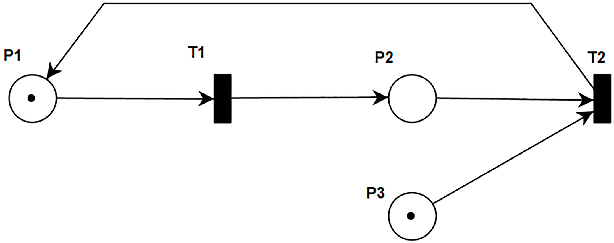
Figure 1 is a simple net containing all components of a Petri Net. There are two types of nodes: places and transitions. Places are represented by circles. Inside the places are tokens, drawn as black dots, which represent the specific value of a condition or object. A particular arrangement of the tokens across all the places is known as a marking or state. The system begins in some initial configuration known as the initial marking. Transitions, represented by rectangles, are used to describe events that may modify the system state. For example, in the Petri Net shown in Figure 1, place $\mathrm{P}1$ and place $\mathrm{P}3$ both have one token, while place $\mathrm{P}2$ has zero tokens. The state of the net is given by the marking of the net, which is given by the number of tokens in the places. The initial marking of the Petri net from Figure 1 is $M_0=[1,0,1]$. In this class of Petri Nets, all the transitions are immediate, i.e., once they are enabled and fired, the new marking is instantly reached. The arcs of the graph are classified as input arcs (arrow-headed arcs from places to transitions) and output arcs (arrow-headed arcs from transitions to places). For instance, transition $\mathrm{T}2$ takes places $\mathrm{P}2$ and $\mathrm{P}3$ as its input places, while $\mathrm{P}1$ is its output place. Arcs have capacity 1 by default. If other than 1, the capacity is marked on the arc. Places have infinite capacity by default, and transitions have no capacity, and cannot store tokens at all. A transition is enabled when the number of tokens in each of its input places is at least equal to the arc weight going from the place to the transition. This results in a new marking of the net, a state description of all places.

Although classical PNs are easy to analyze, they require more places and transitions to model the behaviour of moderately complex systems, which may give rise to a state explosion problem [48]. At the same time, it is problematic to model time-dependent behavior using classical PNs. To overcome the above mentioned limitations, the original Petri net has seen much advancement. Stochastic Petri Nets (SPN) and Generalized Stochastic Petri Nets (GSPN) are among a few widely used variants in a multitude of disciplines.

GSPN is defined by Bause and Kritzinger [49] based on SPN. GSPN has two types of transitions: immediate transitions (to describe some logical behavior) and timed transitions (to describe the execution of time consuming activities). An exponentially distributed delay is associated with the firing of transition to provide a clear and intuitive formalism for generating Markov processes. GSPN adds the inhibitor arcs to prevent the model from becoming exceedingly large [50].

A GSPN is a 6-tuple $GSPN=(P,T,F,W,M_0,\Lambda )$, where

• $P=({\mathrm{P}}_1,{\mathrm{P}}_2,\dots {\mathrm{P}}_{\mathrm{s}})$ is a finite set of places. Places, drawn as circles, model conditions or objects.
• $T=({\mathrm{T}}_1,{\mathrm{T}}_2,\dots {\mathrm{T}}_{\mathrm{m}})$ is a finite set of transitions. GSPN has two types of transitions: timed transitions, represented by hollow rectangles, and immediate transitions, represented by filled rectangles.
• F is a set of arcs such that $F\subseteq (P\times T)\cup (T\times P)$, which represents the arc connections from places to transitions or transitions to places. In a GSPN, it can have an inhibitor arc from a place to a transition which means the transition cannot fire if there is a token in the place.
• W is a weight function that ranges from 1 to infinity, which represents the number of tokens consumed from a place through an arc or the number of tokens deposited to a place through an arc.
• $M_0$ is the initial marking, which a marking represents the distribution of tokens over the places.
• $\Lambda =({\lambda }_1,{\lambda }_2,\dots ,{\lambda }_m)$ is the set of firing rates associated with the transitions. An enabled transition ${\mathrm{T}}_{\mathrm{i}}$ can fire after an exponentially distributed time delay equals $1/{\lambda }_i$ elapses.

3. Modeling the Transmission of Infectious Diseases Using GSPN

3.1. Infectious Diseases Evolution and Transmission Process

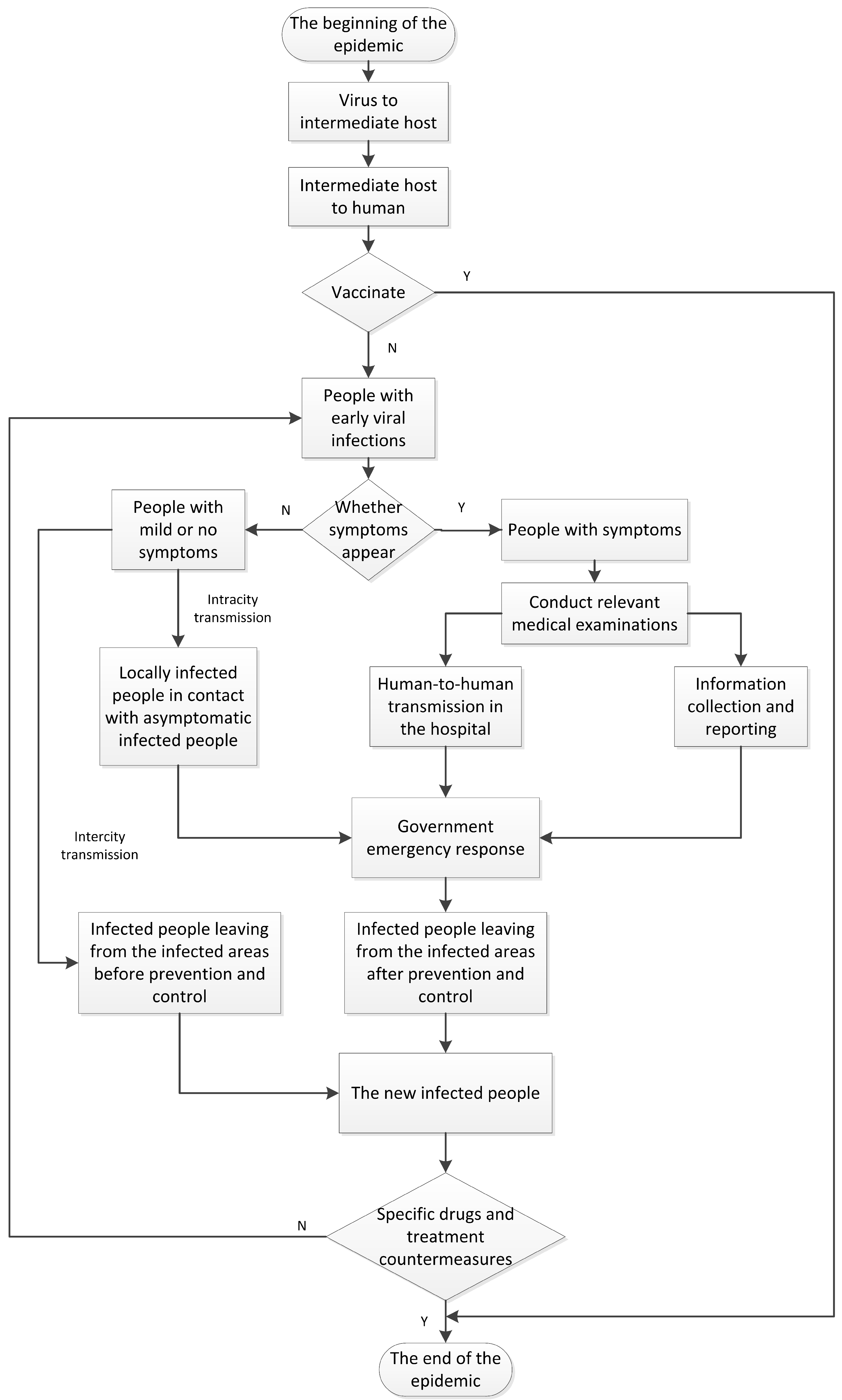
Figure 2 depicts flowchart of the evolution and transmission process of infectious diseases. A completed process consists of three phases as depicted in Figure 2.

The beginning of the infection and immunization phase. The virus first begins to infect intermediate hosts, and then spread from intermediate hosts to the crowd. In this phase, if there is already a vaccine, the virus will not infect people on a large scale. Otherwise, the virus will start to infect people. The development and use of vaccines are key to this process.

The virus spread phase. Because some infectious diseases such as COVID-19 have the characteristics of long incubation period, high infectivity during the incubation period, and carriers with mild or no symptoms which are more likely to cause negligence, this phase includes four parts: the intracity and intercity transmission of asymptomatic infected people, the diagnosis of infected people with symptoms, human-to-human transmission in the hospitals, and epidemic information collection and reporting. The speed of government response and the epidemic prevention response level are critical in this phase. If the governments quickly identify the type and characteristics of the virus and adopt timely quarantine and response measures, they will be able to effectively reduce the infection and spread of the virus.

The development and use of specific drugs phase. The research of specific drugs and effective treatment methods will be an important means to reduce the number of deaths and infected people. As specific drugs research and development will take a relatively long time, in the early stage of virus transmission, blocking the chain of transmission mainly depends on government response measures. When the development of specific medicines is successful, it will be able to effectively suppress the spread of the virus, treat patients, and ultimately stop the epidemic.

3.2. The GSPN-Based General Transmission Model of Infectious Diseases

Based on infectious diseases evolution and transmission process which are shown in Figure 2, we propose the GSPN framework to build the model of the transmission of infectious diseases from the system-level understanding as follows.

• Step 1: Build GSPN model. Define the places, the timed transitions, and the immediate transitions. Estimate the cycle time and obtain the virus spread states.
• Step 2: Generate the reachability graph; it allows us to compute all possible future markings starting from the initial one. Assign each arc with corresponding firing rates, and then generate the homogeneous state-transition Markov chain. All markings are denoted as $M_0,M_1,\dots ,M_{n-1}$, where n is the total number of states. Markings in which at least one immediate transition are enabled are called vanishing markings. On the other hand, markings in which only exponential transitions are enabled are called tangible markings.
• Step 3: Analyze Markov Chain. The obtained reachability graph can be transformed into a Markov model to calculate limiting state probabilities. Next, the steady state probability of tangible markings $P\left[M_i\right]$ can be calculated by solving the equation group as follows:

  $$\begin{array}{c}\hfill P=(P\left[M_0\right],P\left[M_1\right],...,P\left[M_{n-1}\right])\end{array}$$

  (1)

  $$\left\{\begin{array}{c}PQ=0\hfill \\ \sum _{i=0}^{n-1}P\left[M_i\right]=1\hfill \end{array}\right.$$

  (2)

  where n is number of states in the model, $i=\{0,1,\dots ,n-1\}$. P is the state probability vector, and Q is the infinitesimal generator (transition probability matrix). $Q=\left[q_{ij}\right]$, $i=\{0,1,\dots ,n-1\}$ and $j=\{0,1,\dots ,n-1\}$. For the elements $q_{ij}$ outside the main diagonal, if there is an arc from state $M_i$ to state $M_j$, then the value is the firing rate ${\lambda }_k$ of the exponential distribution associated with the transition $T_k$ from $M_i$ to $M_j$; if there is no arc connected, then this element is 0. The element $q_{ii}$ on the main diagonal follows $-\left({\sum }_{i\ne j}{q}_{ij}\right)$ that consequently makes the sum of each row equal to zero.
• Step 4: Analyze and evaluate system performance. After calculating the probability of tangible markings, the token probability density function (PDF) can be calculated which represents the steady state the probability of the number of tokens contained in a place. For a $p_i\in P$, let $P[M_{p_i}=l]$ denote the probability of l tokens contained in place $p_i$, then the token probability density function can be obtained as

  $$\begin{array}{c}\hfill P[M_{p_i}=l]=\sum _{i=0}^{n-1}P[M_i=l]\end{array}$$

  (3)
  The average number of tokens ($U_i$) can be calculated by

  $$\begin{array}{c}\hfill U_i=\sum _{i=0}^{n-1}l\times P[M_{p_i}=l]\end{array}$$

  (4)

  where in the proposed model, $l=0$ or $l=1$ means that all places can only contain 0 or 1 token. The performance of the infectious disease epidemic propagation and evolution system described by GSPN is analyzed and evaluated.

The proposed GSPN model shown in Figure 3 is realized with PIPE tool [51]. In Figure 3, the places, i.e., $\mathrm{P}1$–$\mathrm{P}19$ are drawn as circles, the immediate transitions i.e., T4, T11, T13, T14, T16 are represented by filled rectangles, the timed transitions i.e., $\mathrm{T}1$–$\mathrm{T}3$, $\mathrm{T}5$–$\mathrm{T}10$, $\mathrm{T}12$, $\mathrm{T}15$ are represented by hollow rectangles, and the circle-headed arcs from $\mathrm{P}18$ to $\mathrm{T}3$ and from $\mathrm{P}17$ to $\mathrm{T}14$ are inhibitor arcs.

Table 1. Meanings of places of the GSPN model in Figure 3.

Place	Meaning of Place
$\mathrm{P}1$	The beginning of the virus spread
$\mathrm{P}2$	Intermediate hosts
$\mathrm{P}3$	People with early viral infections
$\mathrm{P}4$	People with symptoms after infection
$\mathrm{P}5$	People with mild or no symptoms after infection
$\mathrm{P}6$	Discovery the new virus
$\mathrm{P}7$	Infected people with symptoms observed in the hospitals
$\mathrm{P}8$	Measures formulated by relevant departments
$\mathrm{P}9$	The new infected people in the hospitals
$\mathrm{P}10$	Locally infected people in contact with asymptomatic infected people
$\mathrm{P}11$	Infected people leaving from the infected areas after prevention and control
$\mathrm{P}12$	Infected people leaving from the infected areas before prevention and control
$\mathrm{P}13$	Infected people moving from infected areas to non-infected areas
$\mathrm{P}14$	Infected people in non-infected areas
$\mathrm{P}15$	Auxiliary place
$\mathrm{P}16$	Start effective treatments and drugs research
$\mathrm{P}17$	Auxiliary place
$\mathrm{P}18$	Complete effective treatments and drugs research
$\mathrm{P}19$	Susceptible population

shows the meanings of places. The meanings and category of transitions are shown in

Table 2. Meanings of transitions of the GSPN model in Figure 3.

Transition	Meaning of Transition	Category
$\mathrm{T}1$	Virus to intermediate hosts	Timed
$\mathrm{T}2$	Intermediate hosts to human transmission	Timed
$\mathrm{T}3$	Whether the infected people have symptoms	Timed
$\mathrm{T}4$	Conduct relevant medical examinations	Immediate
$\mathrm{T}5$	Epidemic information collection and reporting	Timed
$\mathrm{T}6$	Human-to-human transmission in the hospitals	Timed
$\mathrm{T}7$	Human-to-human transmission in the infected areas	Timed
$\mathrm{T}8$	Government emergency response	Timed
$\mathrm{T}9$	Intercity transmission	Timed
$\mathrm{T}10$	Human-to-human transmission in the non-infected areas	Timed
$\mathrm{T}11$	Spread of the virus	Immediate
$\mathrm{T}12$	Successful vaccine development and inoculation	Timed
$\mathrm{T}13$	Auxiliary transition	Immediate
$\mathrm{T}14$	Auxiliary transition	Immediate
$\mathrm{T}15$	Research specific drugs and formulate drug countermeasures	Timed
$\mathrm{T}16$	Treatment of infected people	Immediate

. The overall model depicts the infection process in details, consisting of three phases as follows.

(1) The beginning of the infection and immunization phase. This phase is the process of infection and immunity. $\mathrm{P}1$ is the beginning of the virus spread. $\mathrm{T}1$ represents that the virus starts to infect intermediate hosts. $\mathrm{P}19$ represents the susceptible population. $\mathrm{T}12$ is a timed and key transition that represents whether the vaccine is successfully developed and vaccinated. If all of susceptible people have been vaccinated, the virus will not be able to spread. The token will return to the place of $\mathrm{P}1$. However, if the susceptible people have no vaccine, the virus will start to infect people from intermediate hosts. $\mathrm{T}2$ stands for the virus from intermediate hosts to the people. Because the development of the vaccine needs a relatively long time, the virus will infect people from intermediate hosts. The model will go to the next phase.

(2) The virus spread phase. This phase is the process of the virus spread. $\mathrm{P}3$ represents the infected people. $\mathrm{T}3$ is a timed and key transition that depicts whether the infected people have symptoms. $\mathrm{P}4$ stands for people with symptoms after infection. $\mathrm{P}5$ stands for people with mild or no symptoms after infection.

The immediate transition $\mathrm{T}4$ is enabled when the place $\mathrm{P}4$ contains one token, which represents the fact that people with symptoms have been conducted by relevant medical examinations such as nucleic acid detection. After $\mathrm{T}4$ is fired, the places P6 and P7 will contain a token at the same time, which represents that $\mathrm{P}6$ and $\mathrm{P}7$ occur concurrently. The first process, from $\mathrm{P}6$ through $\mathrm{T}5$ to $\mathrm{P}8$, illustrates the process of discovering new epidemic situation, collecting and reporting the epidemic information, and the government formulating countermeasures. The second process, from $\mathrm{P}7$ through $\mathrm{T}6$ to $\mathrm{P}9$, shows the process of cross-infection between infected and non-infected or medical personnel in the hospitals.

$\mathrm{T}7$ is a timed transition which represents human-to-human transmission in the infected areas. After $\mathrm{T}7$ is fired, $\mathrm{P}10$ and $\mathrm{P}12$ occur concurrently. $\mathrm{P}10$ represents the locally infected people in contact with asymptomatic infected people. $\mathrm{P}12$ represents the infected people leaving from the infected areas before prevention and control. $\mathrm{T}8$ is also a timed and important transition, which indicates that the government has discovered large-scale spread of the virus and has taken corresponding emergency response measures. After $\mathrm{T}8$ is fired, there are two places $\mathrm{P}11$ and $\mathrm{P}15$. $\mathrm{P}11$ stands for the infected people leaving from the infected areas after prevention and control. $\mathrm{P}15$ is an auxiliary place, which means that the GSPN model goes to the development and use of special drugs phase. $\mathrm{T}9$ represents that the infected people move freely between the cities. The process, from $\mathrm{T}9$ through $\mathrm{P}13$, $\mathrm{T}10$, $\mathrm{P}14$, $\mathrm{T}11$ return to $\mathrm{P}3$, illustrates the infected people moving from infected areas to non-infected areas. The virus begins to spread from city to city. This process will be a rapid growth in the number of infected people.

(3) The development and use of specific drugs phase. This phase describes the process of research and treatment of specific drugs. $\mathrm{T}15$ is a timed and key transition that represents the research of specific drugs and the formulation of drug countermeasures. Because the development of the specific drugs is a relatively long time, $\mathrm{T}15$ is delayed to fire which may lead to the tokens accumulation. Therefore, $\mathrm{P}15$ and $\mathrm{P}17$ are the auxiliary places. $\mathrm{T}13$ and $\mathrm{T}14$ are the auxiliary transitions. They are used to prevent the tokens redundancy. $\mathrm{P}16$ represents to start effective treatments and drugs research. $\mathrm{P}18$ represents to complete effective treatments and drugs research. The inhibitor arc from $\mathrm{P}18$ to $\mathrm{T}3$ describes that the specific drugs will be able to suppress the incidence of infected people. At the same time, $\mathrm{T}16$ is an immediate transition which means the infected people can be cured. The state of model returns to the beginning of $\mathrm{P}1$.

The constructed GSPN model gives the boundary conditions of the system. It can identify the number of possible states of the model. As the token moves, the marking changes. Each marking represents a state of the model. The total possible markings represents the total possible states which can be shown as a $M_i\times P_s$ matrix. For the GSPN model of the transmission of infectious diseases in Figure 3, there are $i=40$ states and $s=19$ places, and the state reachable graph can be shown as a $40\times 19$ large matrix. To simplify the matrix representation, in

Table 3. The total possible markings of the GSPN model in Figure 3.

Type	Markings	The Places Having a Token
Tangible markings	$M_0$	($\mathrm{P}1$)
	$M_1$	($\mathrm{P}2$, $\mathrm{P}19$)
	$M_2$	($\mathrm{P}3$)
	$M_4$	($\mathrm{P}5$, $\mathrm{P}6$, $\mathrm{P}7$)
	$M_5$	($\mathrm{P}5$, $\mathrm{P}7$, $\mathrm{P}8$)
	$M_6$	($\mathrm{P}5$, $\mathrm{P}8$, $\mathrm{P}9$)
	$M_7$	($\mathrm{P}8$, $\mathrm{P}9$, $\mathrm{P}10$, $\mathrm{P}12$)
	$M_9$	($\mathrm{P}11$, $\mathrm{P}12$, $\mathrm{P}16$, $\mathrm{P}17$)
	$M_{10}$	($\mathrm{P}11$, $\mathrm{P}12$, $\mathrm{P}17$, $\mathrm{P}18$)
	$M_{11}$	($\mathrm{P}13$, $\mathrm{P}17$, $\mathrm{P}18$)
	$M_{14}$	($\mathrm{P}13$, $\mathrm{P}16$, $\mathrm{P}17$)
	$M_{16}$	($\mathrm{P}3$, $\mathrm{P}16$, $\mathrm{P}17$)
	$M_{18}$	($\mathrm{P}5$, $\mathrm{P}6$, $\mathrm{P}7$, $\mathrm{P}16$,$\mathrm{P}17$)
	$M_{19}$	($\mathrm{P}5$, $\mathrm{P}7$, $\mathrm{P}8$, $\mathrm{P}16$, $\mathrm{P}17$)
	$M_{20}$	($\mathrm{P}8$, $\mathrm{P}9$, $\mathrm{P}10$, $\mathrm{P}12$, $\mathrm{P}16$,$\mathrm{P}17$)
	$M_{22}$	($\mathrm{P}8$, $\mathrm{P}9$, $\mathrm{P}10$, $\mathrm{P}12$, $\mathrm{P}17$, $\mathrm{P}18$)
	$M_{24}$	($\mathrm{P}5$, $\mathrm{P}8$, $\mathrm{P}9$, $\mathrm{P}17$, $\mathrm{P}18$)
	$M_{25}$	($\mathrm{P}7$, $\mathrm{P}8$, $\mathrm{P}10$, $\mathrm{P}12$, $\mathrm{P}16$, $\mathrm{P}17$)
	$M_{26}$	($\mathrm{P}5$, $\mathrm{P}7$, $\mathrm{P}8$, $\mathrm{P}17$, $\mathrm{P}18$)
	$M_{27}$	($\mathrm{P}5$, $\mathrm{P}6$, $\mathrm{P}9$, $\mathrm{P}16$, $\mathrm{P}17$)
	$M_{28}$	($\mathrm{P}5$, $\mathrm{P}6$, $\mathrm{P}9$, $\mathrm{P}17$, $\mathrm{P}18$)
	$M_{29}$	($\mathrm{P}6$, $\mathrm{P}9$, $\mathrm{P}10$, $\mathrm{P}12$, $\mathrm{P}17$, $\mathrm{P}18$)
	$M_{30}$	($\mathrm{P}6$, $\mathrm{P}9$, $\mathrm{P}10$, $\mathrm{P}12$, $\mathrm{P}16$, $\mathrm{P}17$)
	$M_{31}$	($\mathrm{P}5$, $\mathrm{P}8$, $\mathrm{P}9$, $\mathrm{P}16$, $\mathrm{P}17$)
	$M_{32}$	($\mathrm{P}6$, $\mathrm{P}7$, $\mathrm{P}10$, $\mathrm{P}12$, $\mathrm{P}16$, $\mathrm{P}17$)
	$M_{33}$	($\mathrm{P}6$, $\mathrm{P}7$, $\mathrm{P}10$, $\mathrm{P}12$, $\mathrm{P}17$, $\mathrm{P}18$)
	$M_{34}$	($\mathrm{P}5$, $\mathrm{P}6$, $\mathrm{P}7$, $\mathrm{P}17$, $\mathrm{P}18$)
	$M_{35}$	($\mathrm{P}7$, $\mathrm{P}8$, $\mathrm{P}10$, $\mathrm{P}12$)
	$M_{37}$	($\mathrm{P}6$, $\mathrm{P}9$, $\mathrm{P}10$, $\mathrm{P}12$)
	$M_{38}$	($\mathrm{P}6$, $\mathrm{P}7$, $\mathrm{P}10$, $\mathrm{P}12$)
	$M_{39}$	($\mathrm{P}7$, $\mathrm{P}8$, $\mathrm{P}10$, $\mathrm{P}12$, $\mathrm{P}17$, $\mathrm{P}18$)
Vanishing markings	$M_3$	($\mathrm{P}4$, $\mathrm{P}5$)
	$M_8$	($\mathrm{P}11$, $\mathrm{P}12$, $\mathrm{P}15$)
	$M_{12}$	($\mathrm{P}14$, $\mathrm{P}17$, $\mathrm{P}18$)
	$M_{13}$	($\mathrm{P}3$, $\mathrm{P}17$, $\mathrm{P}18$)
	$M_{15}$	($\mathrm{P}14$, $\mathrm{P}16$, $\mathrm{P}17$)
	$M_{17}$	($\mathrm{P}4$, $\mathrm{P}5$, $\mathrm{P}16$, $\mathrm{P}17$)
	$M_{21}$	($\mathrm{P}11$, $\mathrm{P}12$,$\mathrm{P}15$, $\mathrm{P}16$, $\mathrm{P}17$)
	$M_{23}$	($\mathrm{P}11$, $\mathrm{P}12$, $\mathrm{P}15$, $\mathrm{P}17$, $\mathrm{P}18$)
	$M_{36}$	($\mathrm{P}5$, $\mathrm{P}6$, $\mathrm{P}9$)

, we only list the places that have one token in each state $M_i$. In Table 3, the first column is the types of markings, the second column is the name of the states, and the third column is the serial number of the places having one token. For example, on the second row, ($\mathrm{P}2$, $\mathrm{P}19$) means that the places of $\mathrm{P}2$ and $\mathrm{P}19$ have one token in $M_1$ state and the other places have zero token in $M_1$ state.

Table 4. Transition probability matrix of the GSPN model.

Row	Column	Val	Row	Column	Val	Row	Column	Val
$M_0$	$M_1$	${\lambda }_1$	$M_1$	$M_0$	${\lambda }_{12}$	$M_1$	$M_2$	${\lambda }_2$
$M_2$	$M_3$	${\lambda }_3$	$M_4$	$M_5$	${\lambda }_5$	$M_4$	$M_{36}$	${\lambda }_6$
$M_4$	$M_{38}$	${\lambda }_7$	$M_5$	$M_6$	${\lambda }_6$	$M_5$	$M_{35}$	${\lambda }_7$
$M_6$	$M_7$	${\lambda }_7$	$M_7$	$M_8$	${\lambda }_8$	$M_9$	$M_{10}$	${\lambda }_{15}$
$M_9$	$M_{14}$	${\lambda }_9$	$M_{10}$	$M_{11}$	${\lambda }_9$	$M_{11}$	$M_{12}$	${\lambda }_{10}$
$M_{14}$	$M_{15}$	${\lambda }_{10}$	$M_{16}$	$M_{17}$	${\lambda }_3$	$M_{16}$	$M_{13}$	${\lambda }_{15}$
$M_{18}$	$M_{19}$	${\lambda }_5$	$M_{18}$	$M_{27}$	${\lambda }_6$	$M_{18}$	$M_{32}$	${\lambda }_7$
$M_{18}$	$M_{34}$	${\lambda }_{15}$	$M_{19}$	$M_{31}$	${\lambda }_6$	$M_{19}$	$M_{25}$	${\lambda }_7$
$M_{19}$	$M_{26}$	${\lambda }_{15}$	$M_{20}$	$M_{22}$	${\lambda }_{15}$	$M_{20}$	$M_{21}$	${\lambda }_8$
$M_{22}$	$M_{23}$	${\lambda }_8$	$M_{24}$	$M_{22}$	${\lambda }_7$	$M_{25}$	$M_{20}$	${\lambda }_6$
$M_{25}$	$M_{39}$	${\lambda }_{15}$	$M_{26}$	$M_{39}$	${\lambda }_7$	$M_{26}$	$M_{24}$	${\lambda }_6$
$M_{27}$	$M_{31}$	${\lambda }_5$	$M_{27}$	$M_{28}$	${\lambda }_{15}$	$M_{27}$	$M_{30}$	${\lambda }_7$
$M_{28}$	$M_{24}$	${\lambda }_5$	$M_{28}$	$M_{29}$	${\lambda }_7$	$M_{29}$	$M_{22}$	${\lambda }_5$
$M_{30}$	$M_{29}$	${\lambda }_{15}$	$M_{30}$	$M_{20}$	${\lambda }_5$	$M_{31}$	$M_{20}$	${\lambda }_7$
$M_{31}$	$M_{24}$	${\lambda }_{15}$	$M_{32}$	$M_{25}$	${\lambda }_5$	$M_{32}$	$M_{30}$	${\lambda }_6$
$M_{32}$	$M_{25}$	${\lambda }_{15}$	$M_{33}$	$M_{39}$	${\lambda }_5$	$M_{33}$	$M_{29}$	${\lambda }_6$
$M_{34}$	$M_{26}$	${\lambda }_5$	$M_{34}$	$M_{28}$	${\lambda }_6$	$M_{34}$	$M_{33}$	${\lambda }_7$
$M_{14}$	$M_{11}$	${\lambda }_{15}$	$M_{35}$	$M_7$	${\lambda }_6$	$M_{36}$	$M_6$	${\lambda }_5$
$M_{36}$	$M_{37}$	${\lambda }_7$	$M_{37}$	$M_7$	${\lambda }_5$	$M_{38}$	$M_{35}$	${\lambda }_5$
$M_{38}$	$M_{37}$	${\lambda }_6$	$M_{39}$	$M_{22}$	${\lambda }_6$
$M_0$	$M_0$	$-{\lambda }_1$	$M_1$	$M_1$	$-({\lambda }_2+{\lambda }_{12})$	$M_2$	$M_2$	$-{\lambda }_3$
$M_4$	$M_4$	$-({\lambda }_5+{\lambda }_6+{\lambda }_7)$	$M_5$	$M_5$	$-({\lambda }_6+{\lambda }_7)$	$M_6$	$M_6$	$-{\lambda }_7$
$M_7$	$M_7$	$-{\lambda }_8$	$M_9$	$M_9$	$-({\lambda }_9+{\lambda }_{15})$	$M_{10}$	$M_{10}$	$-{\lambda }_9$
$M_{11}$	$M_{11}$	$-{\lambda }_{10}$	$M_{14}$	$M_{14}$	$-({\lambda }_{10}+{\lambda }_{15})$	$M_{16}$	$M_{16}$	$-({\lambda }_3+{\lambda }_{15})$
$M_{18}$	$M_{18}$	$-({\lambda }_5+{\lambda }_6+{\lambda }_7+{\lambda }_{15})$	$M_{19}$	$M_{19}$	$-({\lambda }_6+{\lambda }_7+{\lambda }_{15})$	$M_{20}$	$M_{20}$	$-({\lambda }_8+{\lambda }_{15})$
$M_{22}$	$M_{22}$	$-{\lambda }_8$	$M_{24}$	$M_{24}$	$-{\lambda }_7$	$M_{25}$	$M_{25}$	$-({\lambda }_6+{\lambda }_{15})$
$M_{26}$	$M_{26}$	$-({\lambda }_6+{\lambda }_7)$	$M_{27}$	$M_{27}$	$-({\lambda }_5+{\lambda }_7+{\lambda }_{15})$	$M_{28}$	$M_{28}$	$-({\lambda }_5+{\lambda }_7)$
$M_{29}$	$M_{29}$	$-{\lambda }_5$	$M_{30}$	$M_{30}$	$-({\lambda }_5+{\lambda }_{15})$	$M_{31}$	$M_{31}$	$-({\lambda }_7+{\lambda }_{15})$
$M_{32}$	$M_{32}$	$-({\lambda }_5+{\lambda }_6+{\lambda }_{15})$	$M_{33}$	$M_{33}$	$-({\lambda }_5+{\lambda }_6)$	$M_{34}$	$M_{34}$	$-({\lambda }_5+{\lambda }_6+{\lambda }_7)$
$M_{35}$	$M_{35}$	$-{\lambda }_6$	$M_{36}$	$M_{36}$	$-{\lambda }_7$	$M_{38}$	$M_{38}$	$-({\lambda }_5+{\lambda }_6)$
$M_{39}$	$M_{39}$	$-{\lambda }_6$

is the transition probability matrix (Q) based on Table 3. Because there are 40 states, the transition probability matrix of the proposed model is a $40\times 40$ very large matrix. Similarly, to simplify the matrix representation, in Table 4, we only list the firing rate if there is an arc from state $M_i$ to state $M_j$. We can obtain the relationship between the state probabilities by retrieving the columns with the same number. For example, the val is ${\lambda }_1$ in the row of $M_0$ and the column of $M_1$, and then it can find $-({\lambda }_2+{\lambda }_{12})$ in the row of $M_1$ and the column of $M_1$, so the relationship between the state $M_0$ and $M_1$ can be obtained as follows:

$$\begin{array}{c}\hfill {\lambda }_1\times P\left[M_0\right]-({\lambda }_2+{\lambda }_{12})\times P\left[M_1\right]=0\end{array}$$

(5)

The steady state probability of tangible markings $P\left[M_i\right]$ can be calculated by solving the equation group according to Formula (2). Then, the token probability density function and the average number of tokens can be calculated by Formulas (3) and (4).

4. Experimental Analysis

By using the proposed GSPN model of infectious diseases, the steady-state probability can be analyzed according to the Markov process, and then the average number of tokens (U) in each place is calculated according to Formula (4). Through analyzing the key transitions including $\mathrm{T}5$, $\mathrm{T}6$, $\mathrm{T}7$, $\mathrm{T}8$, $\mathrm{T}9$, $\mathrm{T}10$, $\mathrm{T}12$, $\mathrm{T}15$, it can find how to change some links to improve the operating efficiency of the entire system. It has important practical significance for improving the efficiency of emergency decision-making for epidemic emergencies. In the experimental analysis, the initial parameters of the firing rates are simulated data, not real infectious disease experimental data. The initial transition firing rates are set as ${\lambda }_4={\lambda }_{11}={\lambda }_{13}={\lambda }_{14}={\lambda }_{16}=\infty$, ${\lambda }_1={\lambda }_2=1$, ${\lambda }_3=5$, ${\lambda }_5=4$, ${\lambda }_6={\lambda }_7={\lambda }_{10}=2$, ${\lambda }_8={\lambda }_9=3$, ${\lambda }_{12}={\lambda }_{15}=1$. In order to display the number of people in each stage of the epidemic evolution, we define that N represents the number unit of the population. The number of people in a place can be calculated by $U\times N$. Note that the value of each ${\lambda }_i$ can correspond to the measured or predicted value of the real data. Therefore, epidemiologists can input the parameters of different infectious diseases such as the reproduction number ($R_0$), the probability of the virus transmission, the probability of contacts, and the proportion of the people, etc. into ${\lambda }_i$ as the firing rates.

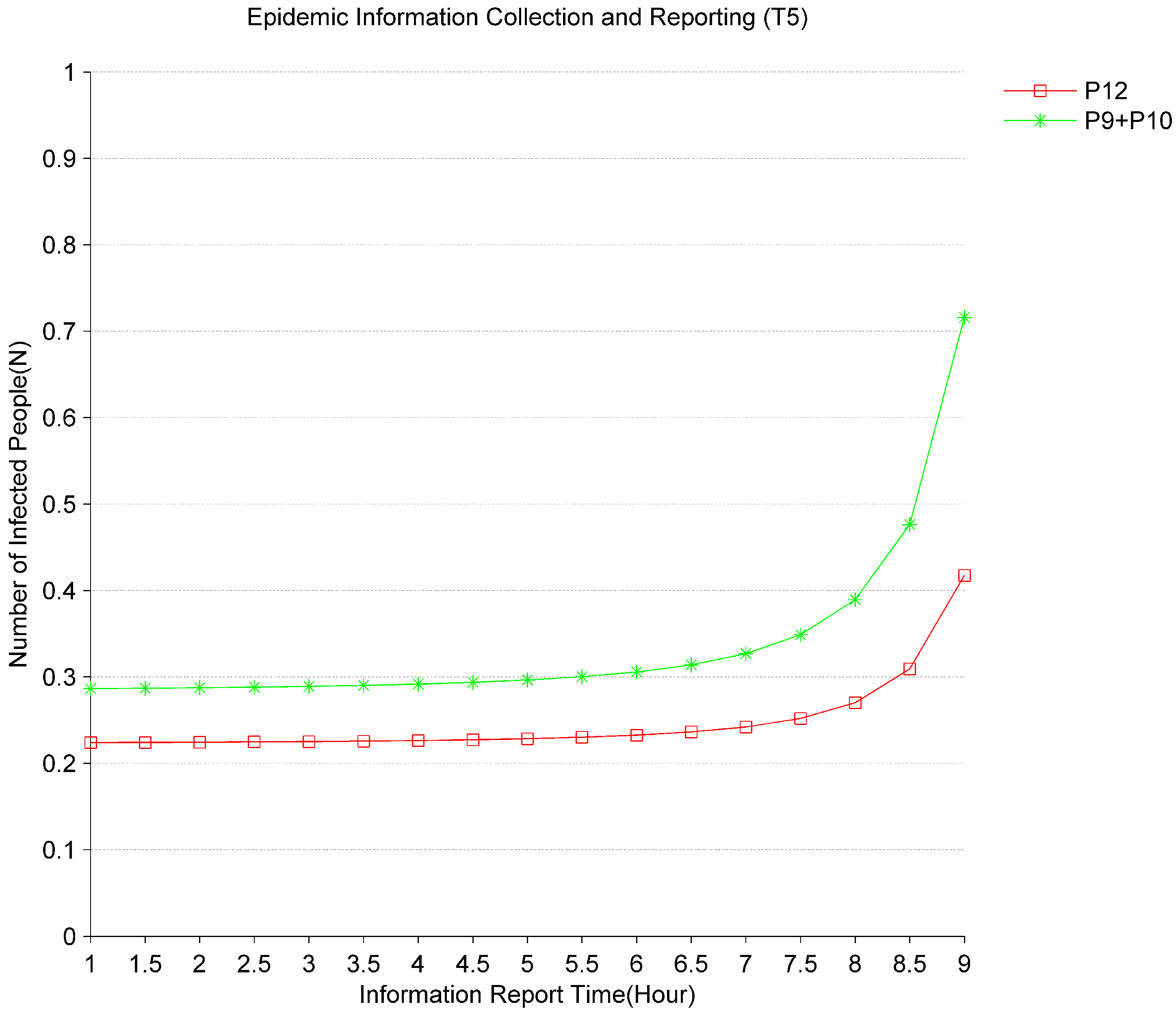
Figure 4 shows the impact of epidemic information reporting time ($\mathrm{T}5$) on the evolution of the epidemic. It can be seen that the sum of the average number of tokens $U\left(9\right)+U\left(10\right)$ in $\mathrm{P}9$ and $\mathrm{P}10$ gradually increases with the delay time of $\mathrm{T}5$ from 1 h to 9 h. The average number of tokens $U\left(12\right)$ in $\mathrm{P}12$ also gradually increases. It indicates that with the longer the time for virus identification and information collection, the speed of virus infection from the initial infected people through hospitals and communities will gradually increase. Especially when the time of $\mathrm{T}5$ is greater than 8 h, the rate of increase in the number of infections in the hospitals and communities will be significantly accelerated. For the social emergency system, it can improve the efficiency of responding to major infectious diseases by speeding up the collection of information on major epidemic diseases and shortening the virus identification cycle.

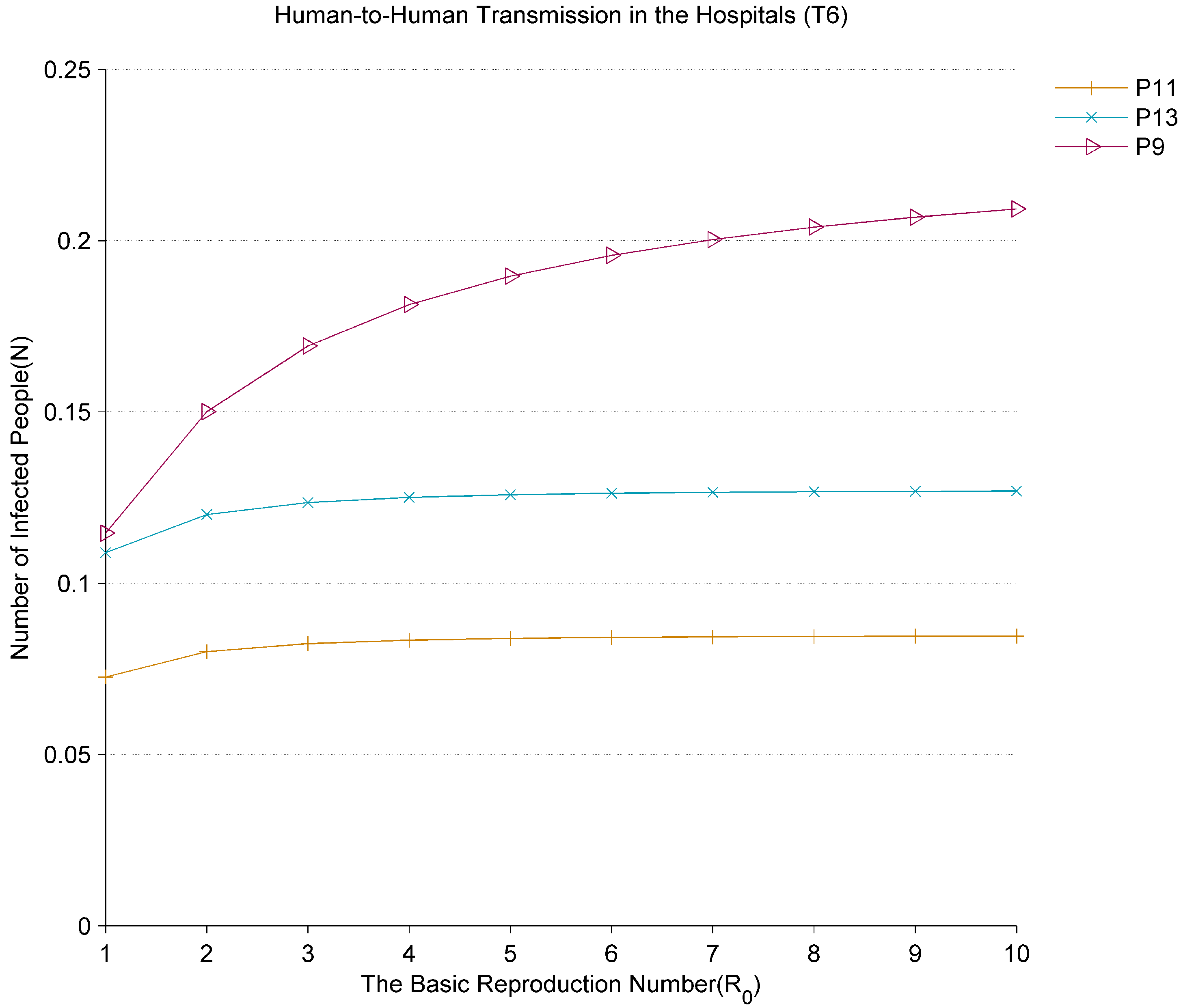
Figure 5 shows the change in the number of infected people in the hospitals with the basic reproduction number ($R_0$). As $R_0$ changes from 1 to 10, the virus spreads faster in the hospitals where the early-onset patients are located. The average number of tokens $U\left(9\right)$ of $\mathrm{P}9$ rapidly increases. It indicates that the new infected people in the hospitals increase significantly with the increase of $R_0$. At the same time, the average number of tokens $U\left(11\right)$ and $U\left(13\right)$ in $\mathrm{P}11$ and $\mathrm{P}13$ will gradually rise with the increasing of $R_0$. This shows that hospital infections are the main source of nosocomial infection to quickly spread the virus to other areas of the community. According to the analysis in Figure 5, as hospitals are places of early contact with infected persons, more attention should be paid to the prevention and control works in hospitals, such as immediately isolating infected patients and avoiding contact with other patients, so as to effectively reduce the transmission rate of the virus and thus curb the spread of the virus in hospitals. Establishing the mobile cabin hospitals in China is the effective way to reduce the rate of nosocomial infections.

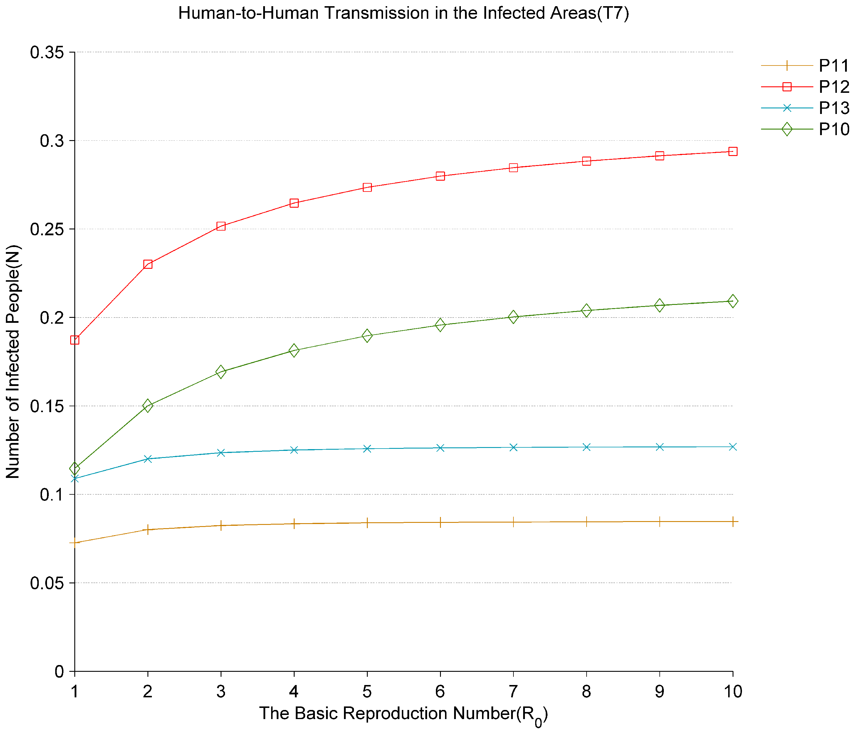
Figure 6 shows the changes in the number of infected people in the infected areas at different values of $R_0$. The mild or no symptoms cases are more likely to cause negligence and accelerate the spread of the virus in the communities. As $R_0$ changes from 1 to 10, the average number of tokens $U\left(10\right)$, $U\left(12\right)$ in the places of $\mathrm{P}10$, and $\mathrm{P}12$ are both rapidly increasing. $\mathrm{P}10$ and $\mathrm{P}12$ are the new infected people inside and outside the infected areas before prevention and control. It indicates that human-to-human transmission in the communities by carriers with mild or no symptoms is the main driving force for the spread of the epidemic. In addition, the average number of tokens $U\left(11\right)$ in the places of $\mathrm{P}11$ is slowly increasing. $\mathrm{P}11$ is the new infected people after prevention and control. It indicates that government emergency response can effectively prevent the output of infected people in the infected areas.

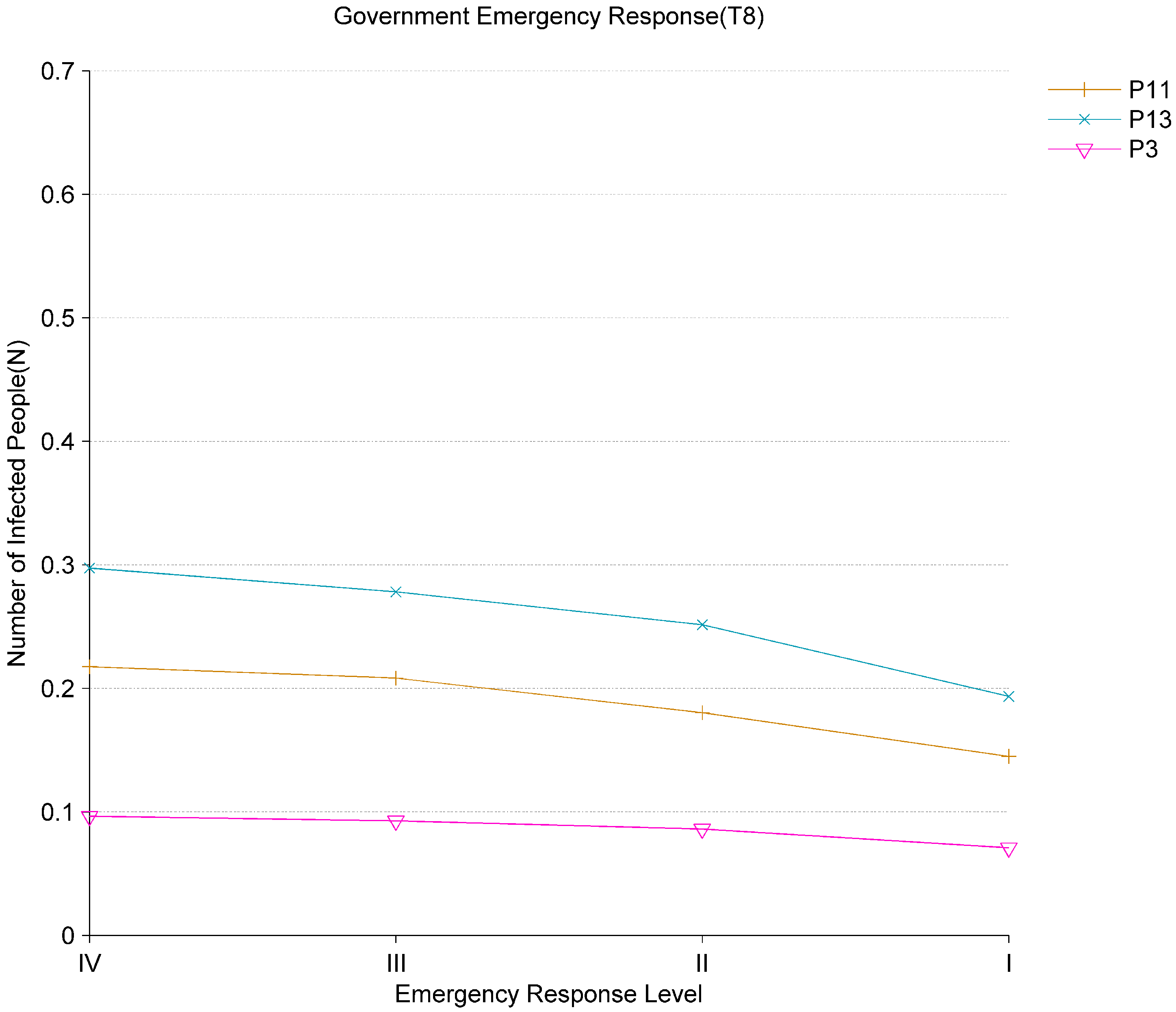
Figure 7 shows the impact of government emergency response ($\mathrm{T}8$) on the evolution of the epidemic. The National Emergency Response Plan for Public Health Emergencies in China stipulates that public health emergencies are classified into four levels including the fourth level ($IV$), the third level ($III$), the second level ($II$), and the first level (I). Level I is the highest epidemic prevention response level. The rise of the response level from level IV to level I means strengthening of epidemic prevention and control measures. The control range and time for the people are expanded, and the crowd mobility is decreased. Based on the analysis of the results in Figure 7, it can find that the mobility of the crowd slows down as the response level increases. The average number of tokens in the places of $\mathrm{P}3$, $\mathrm{P}11$ and $\mathrm{P}13$ all decline. This reflects that the level of government response affects the flow of people, thereby affecting the speed of virus transmission. Because the infectious diseases such as COVID-19 have the characteristics of high infectivity and covert transmission, it is necessary to adopt a higher epidemic prevention response level which can control the wide spread of the virus in the early stage of the outbreak.

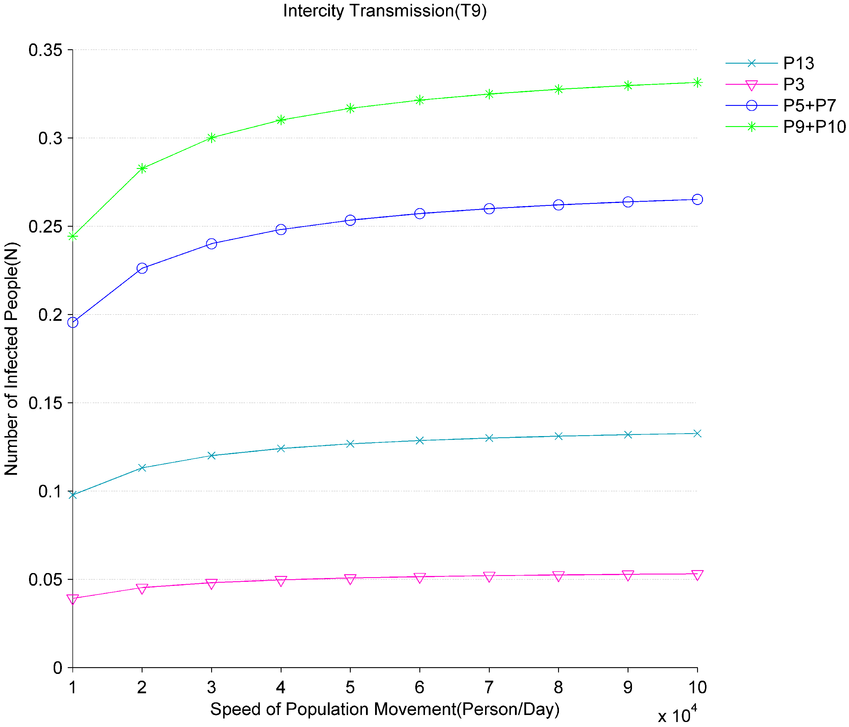
Figure 8 shows the impact of population movement on the spread of the epidemic. Set different values to $\mathrm{T}9$ according to different population movement speed. When the speed of population movement increases from 10,000/day to 100,000/day, the average number of tokens $U\left(13\right)$ in the place of $\mathrm{P}13$ gradually rises. This means that if the population movement between the infected areas and the non-infected areas is not controlled, the infected people in the infected areas will move into the non-infected areas in large quantities. Furthermore, from Figure 8 we can also observe that the average numbers of tokens $U\left(3\right)$, $U\left(5\right)+U\left(7\right)$ and $U\left(9\right)+U\left(10\right)$ in the places of $\mathrm{P}3$, $\mathrm{P}5$, $\mathrm{P}7$, $\mathrm{P}9$, and $\mathrm{P}10$ all go up. This reflects that the newly infected people will form new nosocomial infections and community infections in non-infected areas and result in the spread of the virus between different cities. Therefore, the effective population movement control is an important measure to prevent the spread of the virus. The governments should strengthen the control of population flow after knowing the outbreak of the new virus to prevent the input of infected people from causing the outbreak of the virus locally.

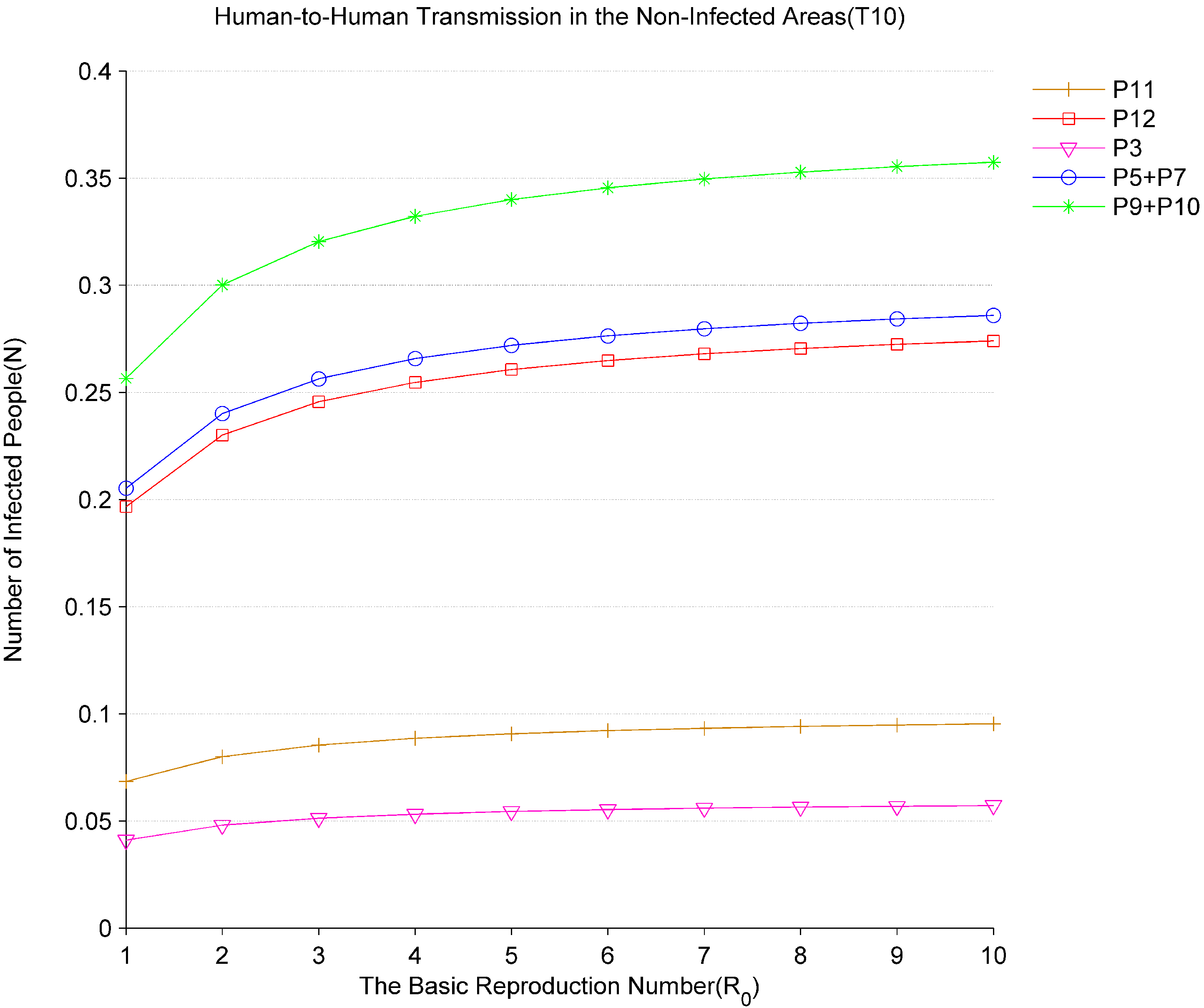
Figure 9 shows the changes in the number of infections in the non-infected areas at different values of $R_0$. $\mathrm{P}3$ denotes the new infected people in the non-infected areas. As $R_0$ changes from 1 to 10, the average numbers of tokens $U\left(3\right)$, $U\left(5\right)+U\left(7\right)$ and $U\left(9\right)+U\left(10\right)$ in the places of $\mathrm{P}3$, $\mathrm{P}5$, $\mathrm{P}7$, $\mathrm{P}9$, and $\mathrm{P}10$ all rise. Based on the analysis of the results in Figure 8 and Figure 9, it can be seen that the speed of population movement and the basic reproduction number are the two important factors that lead to the spread of the virus from the infected areas to the non-infected areas. The governments should actively take measures to detect and treat the infected patients, identify and require people who enter from the virus outbreak areas or have travel history in the infected areas to take self-isolation. These people, as potential sources of transmission, play an important role in virus transmission and control.

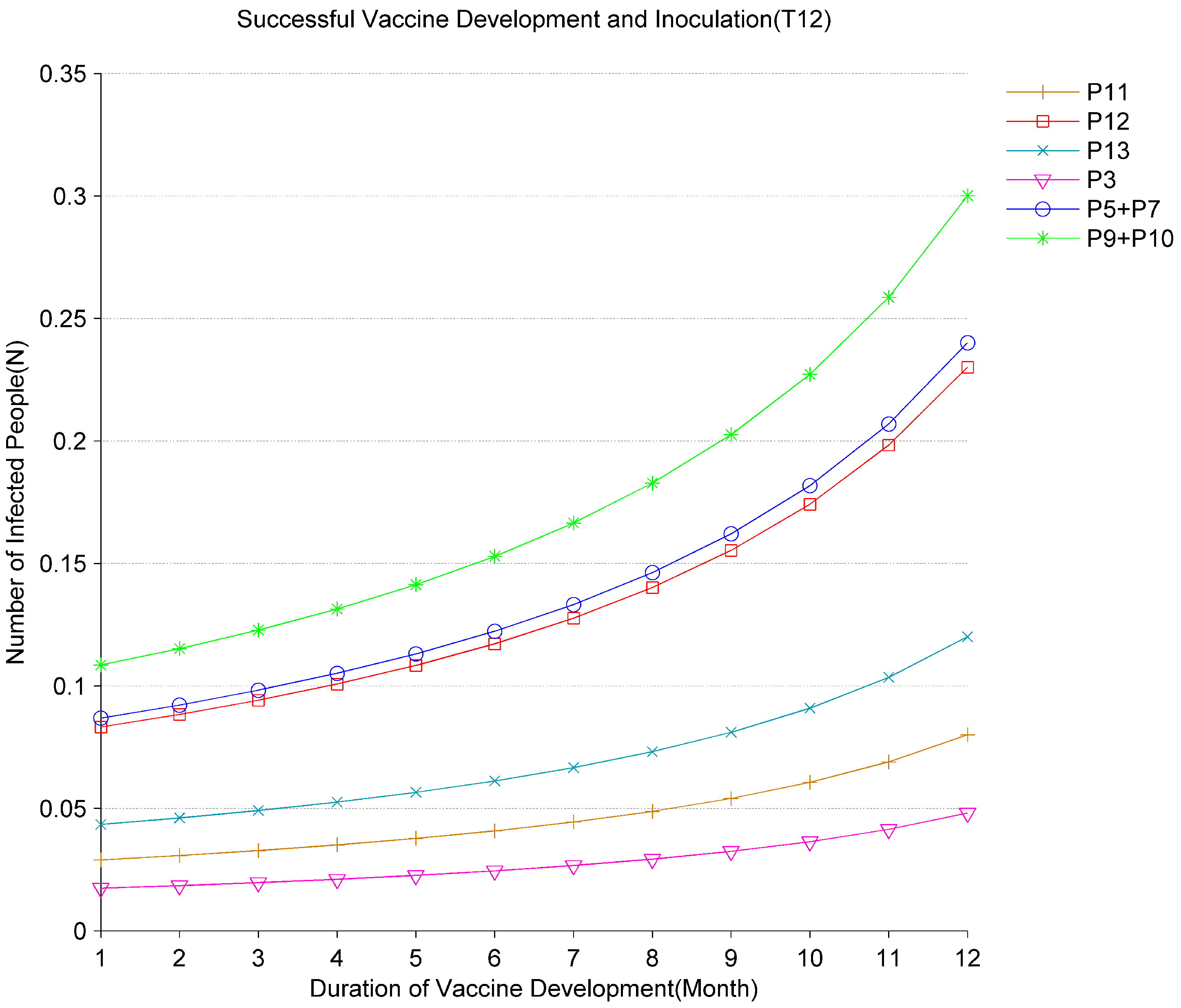
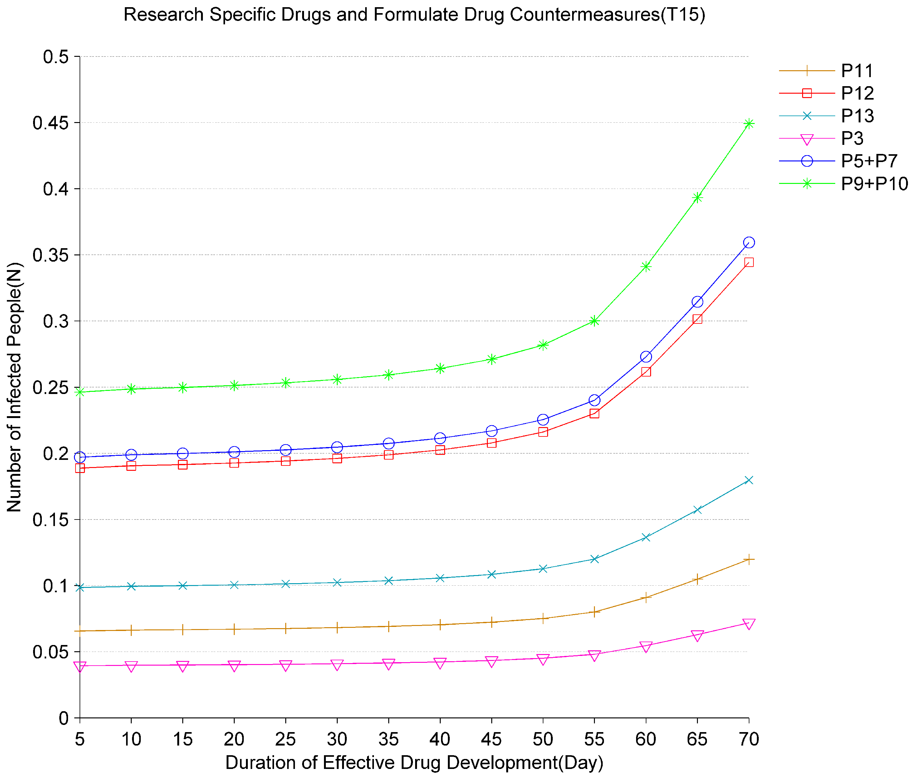
Figure 10 and Figure 11, respectively, show the impact of changes in vaccines and specific drugs development time on the evolution of the epidemic. According to development cycles of different vaccines and specific drugs, different rates for $\mathrm{T}12$ and $\mathrm{T}15$ are set. During the evolution of the epidemic, the vaccine development cycles vary from 1 to 12 months and the specific drugs development cycles vary from 5 to 70 days. Based on the analysis of the results in Figure 10 and Figure 11, the average number of tokens of infected people at $\mathrm{P}11$, $\mathrm{P}12$, $\mathrm{P}13$, $\mathrm{P}3$, $\mathrm{P}5$, $\mathrm{P}7$, $\mathrm{P}9$, $\mathrm{P}10$ has all increased. It indicates that the longer the vaccine and specific drugs development time, the more patients may be infected. Especially after the vaccine development time exceeds 10 months and the specific drugs development time exceeds 55 days, if no other control measures are taken, the number of infected people will accelerate. According to the above analysis, the development of vaccines and specific drugs plays a key role in the final elimination of the virus. The shorter the development cycle is, the fewer infections there are. Therefore, scientists and governments worldwide need to work together to shorten the development cycle and save more patients.

5. Conclusions

Infectious diseases are a major health problem throughout the world. Mathematical models based on an ordinary differential equation (ODE) system have an important role in predicting the outcome of infectious diseases. Markov models for analyzing the dynamics of the spread of epidemics and information have been studied by many researchers. The models based on stochastic Petri nets and their variants are the important evolution of Markov models, which are suitable for modeling the complex and large-scale systems.

In this paper, a new general transmission model of infectious diseases based on the generalized stochastic Petri net (GSPN) is proposed. The advantage of this method is that, with the concurrency and state analysis methods of Petri net, it can analyze the relationship between the associated attribute variables of the development and evolution processes for different events in the infectious disease epidemic event chain. It provides a new analysis model and tool for the infectious disease experts. By setting relevant parameters of different infectious diseases to the firing rates in this Petri model, they can analyze the spread of various diseases, as well as the effect and trend analysis of vaccines, specific drugs, response levels, and restrictions on epidemic control and so on. The experimental results have shown that the proposed GSPN model is an attractive tool and can provide decision support for effective surveillance and response to epidemic development.

In the future work, further cooperations with epidemiologists are needed to map the transmission parameters of various infectious diseases into this model.