Using Convolutional Encoder Networks to Determine the Optimal Magnetic Resonance Image for the Automatic Segmentation of Multiple Sclerosis

Abstract

Multiple Sclerosis (MS) is a neuroinflammatory demyelinating disease that affects over 2,000,000 individuals worldwide. It is characterized by white matter lesions that are identified through the segmentation of magnetic resonance images (MRIs). Manual segmentation is very time-intensive because radiologists spend a great amount of time labeling T1-weighted, T2-weighted, and FLAIR MRIs. In response, deep learning models have been created to reduce segmentation time by automatically detecting lesions. These models often use individual MRI sequences as well as combinations, such as FLAIR${}^2$, which is the multiplication of FLAIR and T2 sequences. Unlike many other studies, this seeks to determine an optimal MRI sequence, thus reducing even more time by not having to obtain other MRI sequences. With this consideration in mind, four Convolutional Encoder Networks (CENs) with different network architectures (U-Net, U-Net++, Linknet, and Feature Pyramid Network) were used to ensure that the optimal MRI applies to a wide array of deep learning models. Each model had used a pretrained ResNeXt-50 encoder in order to conserve memory and to train faster. Training and testing had been performed using two public datasets with 30 and 15 patients. Fisher’s exact test was used to evaluate statistical significance, and the automatic segmentation times were compiled for the top two models. This work determined that FLAIR is the optimal sequence based on Dice Similarity Coefficient (DSC) and Intersection over Union (IoU). By using FLAIR, the U-Net++ with the ResNeXt-50 achieved a high DSC of 0.7159.

1. Introduction

Multiple Sclerosis (MS) is a neuroinflammatory disease that affects over 2,000,000 individuals globally [1]. The disease is accompanied by a very severe phenomenon known as demyelination, which is the degradation of a neuron’s protective myelin sheath [2]. Although the etiology of the disease still needs research, there are clinical procedures that radiologists use to diagnose a patient with MS. Since demyelination can create white matter lesions, one of the most important steps in many diagnostic procedures is to analyze these white matter lesions from magnetic resonance images (MRIs) through a process known as segmentation. The goal of segmentation is to facilitate the diagnosis of the disease and to improve the treatment process.

However, there are multiple types of MRIs that radiologists use for the segmentation and diagnosis of MS [3]. These types of MRIs are often referred to as distinct MRI sequences or MRI modalities. Different MRI sequences can be created by manipulating certain parameters in the settings of an MRI scanner, which is determined by a clinical technician. These MRI sequences look distinct even though they can be representations of the same brain.

A significant issue with current diagnostic procedures is that there is a large amount of ambiguity and no gold standard with respect to an MRI sequence for the segmentation of this disease [4]. Due to this, many radiologists use T1-weighted, T2-weighted, and FLAIR sequences for segmentation. However, current methods of manual segmentation are already fairly time intensive [5]; thus, the time required to obtain multiple sequences adds unnecessary delays in the overall pipeline for segmenting a patient’s lesions.

Therefore, the key contributions of this work come from the process used in determining an optimal MRI sequence. Most studies have not tried to find an optimal sequence for their models [6] and have, thus, not accounted for the time that would come from obtaining the MRIs in a realistic clinical setting. Although there are a few studies that have investigated discrepancies among different MRI sequences, the majority of these studies use a single model in their methodology [7]. This raises a significant question since there is no guarantee that those results would apply to a robust model that might interpret or use features very differently. Hence, the most significant contribution of this work is that it uses different models to ensure that discrepancies in performances are directly attributed to the MRI sequences.

Additionally, this work also focuses on Convolutional Encoder Networks (CENs), which are CNNs that replace the regular encoding pathway with a preexisting encoder. Encoders are networks that solely downsample the input image and extract its features, usually for the purpose of classification. In this work, the decoding pathways of the U-Net, U-Net++, Linknet, and Feature Pyramid Network (FPN) were combined with the ResNeXt-50 encoder. To the best of the authors’ knowledge, this is the first work to use these model combinations specifically for the automatic segmentation of MS.

2. State of the Art

In response to the time intensive nature of segmentation, many deep learning models have been developed in order to improve upon the current clinical methods. Deep learning models are a popular group of nonlinear methods that have greatly improved the state of the art in audio, medical image processing and a wide array of other fields [8,9]. One of these improvements lie within segmentation.

2.1. Convolutional Neural Networks

Convolutional Neural Networks (CNNs) are a type of deep learning model that have been extensively used in the classification of images. In the context of MS, these models function by extracting features and upsampling those features to obtain lesion predictions in the same space of the input image. This process is often referred to as downsampling/encoding followed by upsampling/decoding. A very popular CNN for the segmentation of biomedical images is the U-Net [10], which uses downsampling and upsampling steps that are accompanied by skip connections. This model was created for the segmentation of 2D images, but recent studies have used a 3D model based on the original U-Net. The 3D U-Net has been shown to perform very well, especially for the automatic segmentation of MS [11]; however, it is important to note that it is relatively more expensive with regards to computational resources and memory [12].

Another variation of the U-Net uses a mechanism known as attention to increase the robustness of segmentation performance [13]. It has been shown to perform better than the original U-Net in pancreas, spleen and kidney segmentation [13]. Recently, the attention mechanism has also been used by a model known as the Focus U-Net, which has been used for polyp segmentation [14]. Additionally, a recent model known as the E-Net has been proposed as an alternative to the U-Net because of its fast inference and high accuracy despite requiring less data and fewer computational resources [15]. It has outperformed the U-Net in a variety of different biomedical imaging experiments: the segmentation of the aneurysmal ascending aorta in CT [16], the segmentation of lungs in CT [17], the segmentation of prostates in MR [18], and the segmentation of whole gland and zonal prostates in MR [19].

2.2. Generative Adversarial Networks

Generative Adversarial Networks (GANs) have become another very popular type of deep learning model for segmentation and image processing. Most GANs consist of two different subnetworks known as the ’generator’ and the ’discriminator.’ The goal of the generator is to create images, often using noise vectors, such that the discriminator would not be able to tell the difference between real and ’generated’ images.

Many variations of this framework have been adapted and utilized for biomedical image segmentation. One such example is the MS-GAN [20]. It is a conditional GAN which uses MRIs such as FLAIR and T1 contrast images in place of noise vectors. Another example is the Medical Anomaly Detection GAN (MADGAN) [21], which also takes advantage of the aforementioned attention mechanism. Although this model is used for classification, a recent study has shown its very pertinent applications in both MRI reconstruction and lesion detection [21].

3. Methodology

3.1. Virtual Environment

All code had been executed in Google Colab notebooks with several imported PyTorch libraries [22,23,24]. The virtual environment used within this work operated under 25 GB of RAM and an NVIDIA Tesla V100 GPU.

3.2. Data Acquisition

Two different publicly available datasets had been used in this work. Thirty patients had come from a novel public dataset from the University Medical Center of Ljubljana (UMCL) [25]. Another 15 patients had come from the MSSEG 2016 challenge training dataset [26], as the testing dataset had not been available. Although the combined dataset had a variety of different scanners, there were only 5 patients for each of the MSSEG 2016 scanners, and the overall sample size had only been 45 patients (

Table 1. Dataset Description.

Dataset	Scanners	Patients
UMCL [25]	Siemens Magnetom Trio 3T	30
MSSEG 2016	Siemens Verio 3T	5
	Siemens Aera 1.5T	5
	Philips Ingenia 3T	5

).

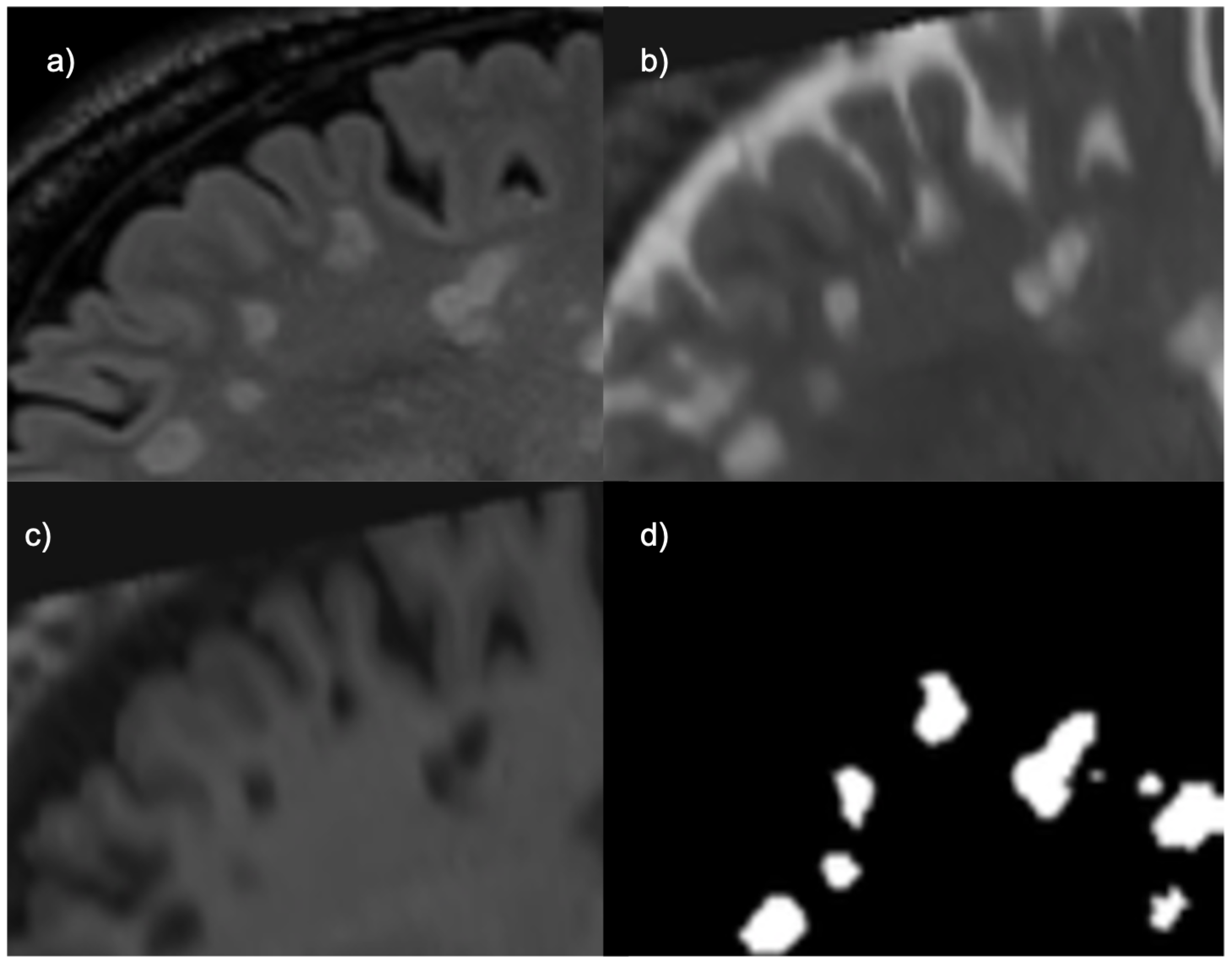
For the UMCL patients, there were three available contrasts: 2D T1, 2D T2, and 3D FLAIR. The lesions in each of these sequences are depicted differently, as shown by Figure 1. FLAIR and T2 MRIs portray lesions as hyperintensities (brighter spots) while T1 MRIs portray them as hypointensities (darker spots). The T1 sequences had been obtained with turbo inversion recovery magnitude, a repetition time (TR) of 2000 ms, an echo time (TE) of 20 ms, an inversion time (TI) of 800 ms, a flip angle (FA) of 120${}^{°}$, and a voxel size of 0.42 × 0.42 × 3.30 mm${}^3$. Each T2 sequence had been obtained with turbo spin echo, a TR of 6000 ms, a TE of 120 ms, an FA of 120${}^{°}$, and a voxel size of 0.57 × 0.57 × 3.00–3.30 mm${}^3$. Each FLAIR sequence had been obtained with a TR of 5000 ms, a TE of 392 ms, a TI of 1800 ms, an FA of 120${}^{°}$, and a voxel size of 0.47 × 0.47 × 0.80 mm${}^3$. Each image came in 192 × 512 × 512 volumes, with the exception of patient 11 whose image came in a volume with dimensions 176 × 512 × 512.

For the MSSEG 2016 dataset, three scanners were used to obtain a sagittal 3D FLAIR image, sagittal 3D T1 image, and an axial 2D T2 image. The acquisition details for this dataset are shown in

Table 2. MSSEG 2016 MRI Acquisition Description.

Scanners	Sequence	Volume Dimension	Voxel Resolution (mm³)
Siemens Verio 3T	FLAIR	144 × 512 × 512	0.5 × 0.5 × 1.1
	T1	176 × 256 × 256	1 × 1 × 1
	T2	44 × 240 × 320	0.69 × 0.69 × 3
Siemens Aera 1.5T	FLAIR	128 × 256 × 224	1.03 × 1.03 × 1.25
	T1	176 × 256 × 256	1.08 × 1.08 × 0.9
	T2	25 × 320 × 320	0.72 × 0.72 × 4 Gap: 1.2
Philips Ingenia 3T	FLAIR	261 × 336 × 336	0.74 × 0.74 × 0.7
	T1	200 × 336 × 336	0.74 × 0.74 × 0.85
	T2	46 × 512 × 512	0.45 × 0.45 × 3

.

The ground truth for the UMCL dataset had been created by consensus among three different raters (Figure 2), and the ground truth for the MSSEG 2016 dataset had been created using segmentations from seven different raters. Since the presence of more expert raters creates higher intervariability, the creators of the MSSEG 2016 dataset had used the Logarithmic Pool Based STAPLE algorithm to provide a consensus ground truth [26].

3.3. Preprocessing

Both datasets had already been preprocessed with bias correction and the registration of each image in FLAIR space. Skull stripping was applied on the UMCL dataset since the MSSEG 2016 MRIs had already been skull stripped. Further preprocessing of the data was performed on each MRI by applying visual transformations on both the mask and corresponding modality. Each slice had been resized to a shape of 224 × 224 to standardize the input dimensions. It is important to note that sagittal slices were used because most volumes would not yield square images otherwise. For example, an MRI volume with the shape 192 × 512 × 512 would yield an image shape of 192 × 512 if the axial (transverse) or coronal slices had been used instead.

3.4. Models Used

As stated earlier, four different CENs were used: ResNeXt-50 with FPN, ResNeXt-50 with Linknet, ResNeXt-50 with U-Net, and ResNeXt-50 with U-Net++.

The U-Net model was proposed for biomedical image segmentation [10], and it is among some of the current state-of-the art methods. It functions by the same logic of basic encoder-decoder pathways, except with this model the decoding pathway consists of unique up-convolution layers to scale the feature maps to a readable output segmentation.

The U-Net++ was proposed after the introduction of the U-Net model [27]. It was created to improve upon the U-Net’s segmentation performance by increasing the number of skip connections. By using more intermediate skip connections, the U-Net++ can extract finer details in features that may not be accounted for in the normal U-Net; this is very important in the context of biomedical imaging since fine details often correspond to significant biomarkers [27,28].

The Feature Pyramid Network (FPN) is a network architecture that uses features in a different manner than the aforementioned models [29]. For FPNs, the model generates a series feature maps with decreasing size and stacks them in a pyramid shape. These feature maps are then converted into actual predictions using an activation function. These predictions are compiled into a final segmentation output image by using the sums of each tier within the feature pyramid.

The Linknet model is considered to be a relatively fast and efficient model for segmentation [30]. Generally speaking, it is also the lightest out of these four in terms of the actual architecture. Although this model does not have as many layers as the aforementioned models, previous studies have shown that for other segmentation tasks, excluding biomedical segmentation including MS, the model has been able to yield relatively good performances [31].

Encoder

Each of these models had the same ResNeXt-50 encoder [32] backbone trained on ImageNet [33] weights in order to allow for faster training. This also eliminates the chance that discrepancies within performances could be attributed to differences in feature extraction. By controlling for the encoder, performances are dependent on how a model used extracted features. Thus, the optimal MRI sequence would yield the best performance depending on how a model upsamples extracted features.

It is important to clarify that the ResNeXt-50 encoder consists of 6 scales (original, 1/2, 1/4, 1/8, 1/16, and 1/32), while the original U-Net decoding pathway consists of 5 scales (original, 1/2, 1/4, 1/8, and 1/16). For this reason, the decoding pathway of the U-Net had an additional scale (1/32) to account for the skip connections for each of the ResNeXt-50 feature maps except for the original (Figure 3). These scales had applied to the U-Net++ as well; thus, there were more intermediate skip connections appended to account for the extra scales.

The ResNeXt-50 encoding pathway uses a 7 × 7 convolutional layer with a stride of 2 to create the first feature map. This is why the original input image is not used for a skip connection; however, this would be an interesting avenue for future research if one were to include the image of original scale in a skip connection for this specific model. Afterwards, each encoder step had used residual blocks, which had consisted of a 1 × 1 convolutional layer, a 3 × 3 convolutional layer, and a 1 × 1 convolutional layer [32].

In Figure 3, each decoding step on the right hand is performed by two 3 × 3 convolutional layers and ReLU activation, which compose the decoding pathway of the original U-Net model. These convolutional steps were also present in the U-Net++ decoding pathway, but the inclusion of the 1/32 scale allowed for the creation of additional sets of skip connections. The decoding pathway of the FPN uses a 3 × 3 convolutional layer with ReLU activation on the feature map with the smallest scale and a 1 × 1 convolution for the next three scales [29]. This had output feature maps of four different scales with 256 channels. This meant that in order to use the actual FPN decoding pathway, all six encoder scales could not have a corresponding skip connection. The feature maps of scales 1/32, 1/16, 1/8, and 1/4 were used for top down merging as part of the decoding pathway. The decoding pathway of the Linknet is characterized by a series of decoding blocks that are composed of a 1 × 1 convolution, a 4 × 4 transpose convolution with stride of 2, and a final 1 × 1 convolution [30]. For this model the skip connections of the decoding pathway had used the feature maps of scales 1/32, 1/16, 1/8, 1/4, and 1/2. This was because the first step of the ResNeXt-50 did not produce a feature map of original scale, as mentioned earlier.

3.5. Experiments

Although the dataset had been limited even with the utilization of different publicly available datasets, 2D wise segmentation had meant that the models could iterate through volumes of MRI data. This had greatly increased the actual training data to approximately 8000 slices. In addition, the FLAIR${}^2$ multi-contrast combination had been considered in this work. This input combination is simply the result of multiplying the FLAIR and T2 sequences, and it has been shown to provide better lesion contrast, albeit when using a different scanner [34].

Training and testing had been performed multiple times. The first time had been with the UMCL dataset, and the second time had been with the combined dataset. The results obtained during the first experiment were used to determine an optimal MRI sequence. In order to thoroughly assess the inter-scanner applications of these sequences and FLAIR${}^2$, the second experiment used 5-fold cross validation, given that there were only five patients from each scanner from the MSSEG 2016 dataset.

3.6. Training (UMCL Dataset)

Each model trained for 25 epochs with a batch size of 16. Eighteen randomly sampled patients were used for training, and another six randomly sampled patients had been used for internal validation (fine-tuning). This provided a roughly 75/25 percentage split of the data during the training step.

Training had been performed by iterating through 2D slices of patient MRI volumes to conserve memory. The RAdam optimizer [35] had been used along with the Lookahead algorithm to improve the learning stability with very little memory cost [36]. During training, the state of each model had been saved after each epoch so that the model would load its optimal state before testing. For example, if a given model had started to diminish in performance towards the end of its training, the version of the model from an earlier epoch would be used. This was performed in order to reduce the potential impact of over fitting and to evaluate each model using their optimal states.

3.6.1. Dice Similarity Coefficient and Intersection over Union

Accuracy in classification tasks can be useful if the dataset evenly distributes the instances of each class. However, since the sizes of lesions are very small there are significantly few “lesion” voxels to be accurately classified; this phenomenon is known as class imbalance [37]. Thus, if models were to return predictions of only blank space for some slices of the brain, the accuracy can still be very high. Consequently, this research study evaluates a sequence’s tendency to yield better performances based on the Dice Similarity Coefficient (DSC) and Intersection over Union (IoU).

The DSC is frequently used for evaluating the performance segmentation models. It can be calculated as shown by the equation below.

$$DSC=\frac{2\times TP}{TP+FP+TP+FN}$$

(1)

The IoU is another metric used for evaluating the performance of segmentation models. It is very similar to the DSC, except for the fact that it does not weigh the true positives as much as the DSC. It can be calculated as shown by the equation below.

$$IoU=\frac{TP}{TP+FP+FN}$$

(2)

In general, these metrics are a measure of the extent to which two images are similar by how much they align when they are overlapped; this proves to be useful for evaluating how the input choice can affect segmentation performance. These metrics are able to mitigate the impact of class imbalance because of the greater emphasis on true positives. For this reason, these metrics are used in other research studies.

3.6.2. Loss Function

The loss function is essential to most machine learning pipelines. Usually, a model learns by minimizing its loss, which is derived from the difference between a ground truth sample and a set of predictions. In the case of class imbalance, many studies use Dice loss within the loss function [38]. A recent loss function known as the Tversky loss has also been created to mitigate this problem, but since DSC and IoU were the primary metrics, the loss function had incorporated Dice and IoU loss. However, few studies have shown that models trained on the Tversky Loss function have the potential to yield better segmentation performances if the weighted parameters of the loss function are experimentally determined [39]. Thus, using this function is a very viable future direction.

The loss functions below include Dice loss and IoU loss, which are simply the DSC or IoU subtracted from one.

$$L_{Dice}=1-DSC$$

(3)

$$L_{IoU}=1-IoU$$

(4)

The binary cross entropy (BCE) function, also referred to as the log-loss function, is a standard loss function that is used in binary classification tasks [40]. Although the focus of this work had been on segmentation in lieu of classification, the segmentation process in this context is dependent on evaluating whether any given voxel is a lesion or not, which is a binary task. By using the logarithmic behavior in the BCE, these models had been much more penalized for wrong predictions of a given voxel.

$$L_{BCE}=-\frac{1}{N}\sum _{i=1}^N(y_i\times log\left(p\left(y_i\right)\right)+((1-y_i)\times log\left(p\left(y_i\right)\right)$$

(5)

The DSC and IoU loss functions were weighted and combined with the BCE function to obtain an aggregate loss function.

$$L_{Aggregate}=1.0\times L_{Dice}+1.0\times L_{IoU}+0.8\times L_{BCE}$$

(6)

The purpose of these weights were to allow the models’ loss to correspond directly to the DSC and IoU while still being influenced by the BCE loss but to a lesser extent. The theoretical maximum loss in this case would be infinite because BCE does not have a maximum.

3.7. Testing (UMCL Dataset)

The remaining six patients were used for testing, and the final DSC and IoU scores were averaged. During testing, a lesion was determined to be present if the model was at least 90% confident that a given voxel belonged to a lesion (threshold = 0.9).

3.8. Fisher’s Exact Test

A Fisher’s exact test was performed using a 2 × 2 contingency table. In order to determine if the optimal MRI’s performances had been statistically significant, this table was created to compare how often a model using the optimal sequence outperformed the same model by using the other inputs. Since there were four models each using six patients and four types of inputs, a sample size of 96 outcomes had been used for the contingency table.

3.9. Automatic Segmentation Time

Subsequently, the time it took to segment a patient for the two best models had been recorded for each of the six testing patients. The purpose of this step was to determine how long it would take to segment a patient’s lesions when using the optimal input.

3.10. Training (Combined Dataset)

Training and testing with the combined dataset had been performed by using 5-fold cross validation. The training procedure itself had remained the same: each model trained for 25 epochs, The RAdam optimizer with the Lookahead algorithm was used, and the loss function had still been an aggregate of the BCE, DSC, and IoU loss functions. However, in this case, 36 patients had been used for training, and nine patients had been used for training. This was conducted to yield an 80/20 percentage ratio for each validation fold.

3.11. Testing (Combined Dataset)

Testing had been performed using nine patients of the combined dataset for each fold. In each fold, six of the patients had been from the UMCL dataset, and three of the patients had been from MSSEG 2016 dataset; this was conducted in order to keep the training and testing ratio consistent between both datasets. The final testing metrics are averages of each validation fold. Additionally, the testing predictions of the best model-input combination were visualized as contours over the corresponding MRI in order to qualitatively evaluate the model’s segmentation performance.

4. Results and Discussion

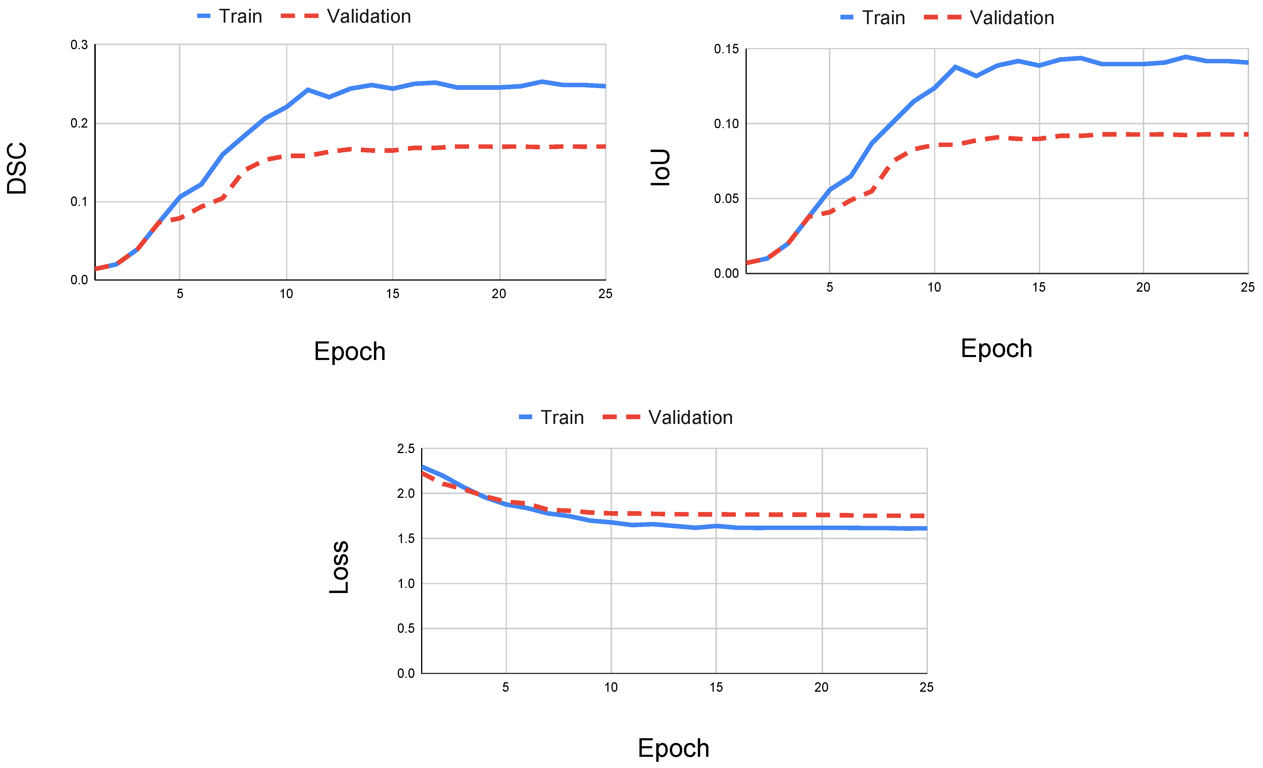
When using only the FLAIR modality, the U-Net with ResNeXt-50 yielded the best performance during training compared to the other models. Since each model had reached asymptotic behavior with respect to the aggregate loss, the DSC, and IoU at the end of the training step, any change or increase in the number of epochs would not change the outcome of training (Figure 4). In some cases, other models had obtained its optimal performance before reaching the last epoch, which indicates that an increase in the epoch size could counteract the training because the model would overfit the training data. Regardless, each model reached higher DSC and IoU scores when using the FLAIR sequence.

Additionally, since the weights that yielded the highest DSC had been saved and used during testing, the testing metrics of the model are reliable for obtaining the optimal performance relative to a particular MRI sequence. However, because the training performance could change based on the amount of data, a larger dataset was considered for subsequent training and testing.

Table 3. Testing Metrics Using UMCL Dataset.

Input	Model	DSC	IoU
T1	FPN	0.5018	0.4835
	Linknet	0.4060	0.3988
	U-Net	0.4972	0.4703
	U-Net++	0.1072	0.1066
T2	FPN	0.5519	0.5277
	Linknet	0.4948	0.4948
	U-Net	0.5612	0.5268
	U-Net++	0.5814	0.5453
FLAIR	FPN	0.6250	0.5851
	Linknet	0.5988	0.5880
	U-Net	0.6678	0.6223
	U-Net++	0.6677	0.6222
FLAIR${}^2$	FPN	0.5153	0.3740
	Linknet	0.5652	0.4105
	U-Net	0.5497	0.3932
	U-Net++	0.5614	0.4038

portrays the DSC and IoU for the four CENs when using each of the different inputs. The DSC and IoU metrics show that the FLAIR sequence yielded the best segmentation performance during testing across all models. When using FLAIR, the U-Net with ResNeXt-50 had obtained a DSC of 0.6678 and an IoU of 0.6223; this indicates that the U-Net CEN with a FLAIR MRI sequence performed the best compared to every other model-sequence combination.

Additionally, models using the FLAIR${}^2$ sequence did not outperform models using the FLAIR sequence. However, they provided better segmentations than when using the T2 sequence. A possible explanation for this could be the result of relying on a single specific scanner. Additionally, a recent study has experimentally found a different multi contrast combination known as FLAIR${}_3$ [41]. This combination is created by multiplying FLAIR${}^{1.55}$× T2${}^{1.45}$, and it has been demonstrated to create higher contrast [41]. Thus, it would be worthwhile to investigate the utilization of FLAIR in future works.

It is important to note the differences between the U-Net++ CEN and the U-Net CEN. In the case of T2 sequences, the U-Net++ outperformed the U-Net with respect to DSC by approximately 0.02 points. However, in the case of T1 sequences, the U-Net++ CEN did much worse relative to the other models with a DSC of 0.1072 and an IoU of 0.1066. When analyzing the training of the U-Net++ CEN using the T1 sequence, both the DSC and IoU plateau and the loss function reaches asymptotic behavior (Figure 5). Thus, it is most likely not the case that training the model with more data could ameliorate the testing performance. A possible explanation for these differences is that the U-Net++ adds more intermediate skip connections with the intent of remedying dissimilar feature maps between the encoding and decoding steps. Hence, the differences in performances can come from discrepancies in upsampling features or the abundance of skip connections. However, skip connections are mainly used for managing gradients during back propagation; thus, it could be dependent on T1 sequences specifically obtained from the scanner used in the UMCL dataset.

Regardless, these data show that the FLAIR MRI sequence has a tendency to yield better performances when used for segmentation. Additionally, when using the FLAIR sequence, the U-Net++ CEN and the U-Net CEN had a marginal difference with respect to DSC (0.0001); this suggests that there is no appreciable difference between these models and that both of them can provide robust segmentation when using the FLAIR MRI sequence.

Since each of the four models tested on six patients with four different MRI sequences, there were a total of 96 different performances.

Table 4. Shown is a contingency table that categorizes a total of 96 distinct model performances. This table shows how often FLAIR achieved the best performance (Rank 1) relative to the other performances (Rank 2, 3, and 4) for the other inputs. A Fisher’s exact test determined that the distribution of model performances was statistically significant (p < 0.00001).

	Rank 1	Rank 2, 3, 4
FLAIR	18	6
Other Inputs	6	66

is a contingency table, which demonstrates how often a model using FLAIR had achieved the best performance (Rank 1) and how often a model using the other inputs did not achieve the best performance. A Fisher’s exact test took the distribution of the performances into account, and it had indicated that these results had been statistically significant. This validates the observed results for the FLAIR MRI sequence during testing and training. Although more performances can be used to further validate these results, based on these data, it holds that the FLAIR MRI sequence is the optimal MRI sequence for automatic segmentation.

Table 5. Final metrics for U-Net and U-Net++ were obtained for each of the six final testing patients.

Model	Time and DSC	1	2	3	4	5	6
U-Net with ResNeXt-50	Time (seconds)	5.6973	5.4851	5.5566	5.5522	5.5916	5.5049
	DSC	0.7105	0.8016	0.4080	0.6495	0.6190	0.8181
U-Net++ with ResNeXt-50	Time (seconds)	5.8920	5.6322	5.6716	5.6639	5.7019	5.7126
	DSC	0.7047	0.7791	0.4095	0.6785	0.6094	0.8250

displays the time it took to segment each patient’s brain and the corresponding DSC for the U-Net and U-Net++ CENs using FLAIR. It is important to note that although the U-Net with ResNeXt-50 had the best average DSC (0.6678), the U-Net++ with ResNeXt-50 had the best case DSC (0.8250) from patient six. However, it is also important to note the high variability among patients, specifically the outlier of patient four. Fortunately, this could be significantly improved with the availability of more patient data. Regardless, both models were capable of achieving very robust segmentations in the range of seconds when using only the FLAIR MRI.

A possible explanation for why the FLAIR MRI sequence yielded the best performance for each of the four models is most likely due to the way the lesions are numerically represented. Since CENs classify based on the number associated with a voxel (higher numbers indicate brighter lesions), they are ultimately classifying based on brightness. Hence, the MRI sequence that depicts lesions the brightest would intuitively yield better performances. However, although FLAIR lesions are darker compared to T2 lesions, FLAIR lesions are surrounded by dark brain matter. This facilitates a CEN in identifying bright lesion voxels among dark background voxels. Additionally, since the T2 sequence often depicts CSF as brightly as hyperintense white matter lesions, it is likely that a given model would have a difficult time differentiating between healthy and diseased brain matter. Although the initial reasoning for using T2 sequences clinically was that lesions could be better identified in the infratentorial sections of the brain [42], these data suggest that the ambiguity of determining a lesion from T2 sequences ultimately give way to better performances with the use of FLAIR sequences in the context of automatic segmentation.

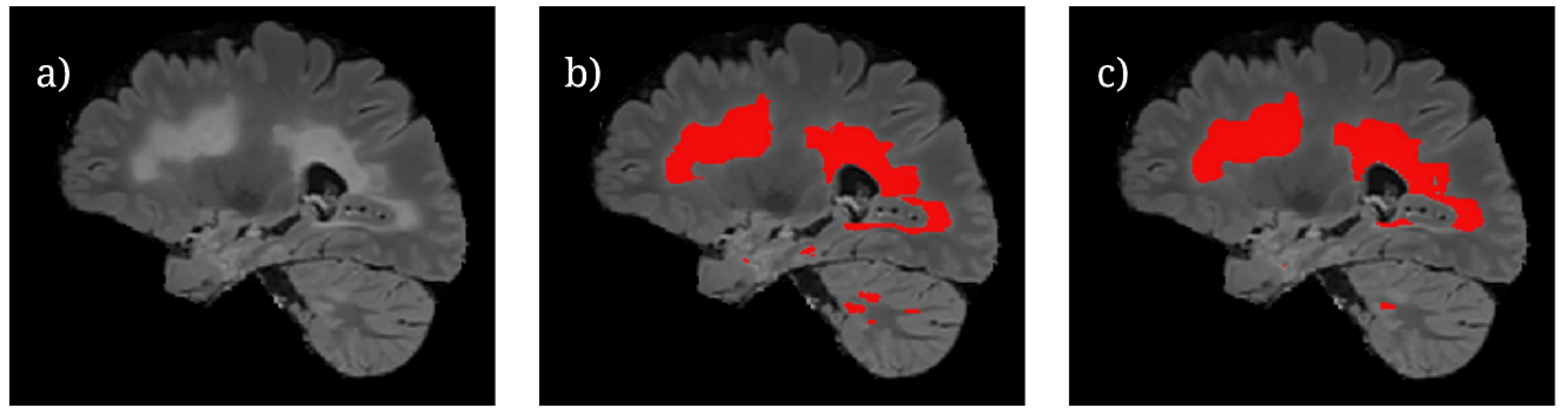
Figure 6 shows the U-Net++ CEN predictions of lesion locations during testing. It is important to note that while larger volumes of lesions are able to be segmented proficiently by the model, there are still differences between the predictions and ground truth for smaller lesion fragments. This is most likely due to the difficulty in classifying small lesion volumes in isolation. A potential avenue of investigation with regards to this observation is to train the model by using specific regions of a brain slice where the lesions are known to be smaller. This is similar to an attention-based model framework which has been known to perform well [13], but it would require significantly more labeled data.

When training and testing using 5-fold cross validation, the models had improved slightly with regards to the DSC (

Table 6. Testing metrics using combined dataset.

Input	Model	DSC	IoU
T1	FPN	0.4585	0.3038
	Linknet	0.4220	0.2730
	U-Net	0.4862	0.3272
	U-Net++	0.5197	0.3571
T2	FPN	0.5336	0.3704
	Linknet	0.5137	0.3513
	U-Net	0.5677	0.4024
	U-Net++	0.6079	0.4423
FLAIR	FPN	0.6246	0.4945
	Linknet	0.6305	0.4646
	U-Net	0.6939	0.5355
	U-Net++	0.7159	0.5612
FLAIR${}^2$	FPN	0.6048	0.4387
	Linknet	0.5991	0.4324
	U-Net	0.6624	0.4996
	U-Net++	0.6743	0.5132

); this is most likely due to the availability of more data from different scanners. However, it is important to note that the IoU had also decreased in a few cases, especially in the case of T1. Based on the DSC of 0.5197 and an IoU of 0.3571, the 5-fold cross validation demonstrates that when using T1, the U-Net++ with ResNeXt-50 can yield better performances than other models using the same sequence. This could mean that the U-Net++ CEN with regards to Table 3 does not have significantly lower performances when using T1; thus, it is more likely the result of the random distribution of data when training and testing with the UMCL dataset. Regardless, this is a something that that could be revisited in future works.

Additionally, FLAIR${}^2$ does not yield better segmentation performances after 5-fold cross validation, but it follows FLAIR relatively closely. This might suggest that the segmentation performances when using this multi-contrast combinations are dependent on the type of scanner used. Based on the performances when using FLAIR, the FLAIR${}_3$ multi-contrast combination could provide a better performance since, technically, the FLAIR exponent (1.55) is slightly more than the T2 exponent (1.45).

5. Conclusions and Future Works

This work used different CENs to determine the optimal MRI sequence for the automatic segmentation of MS. The utilization of CENs with different decoding pathways was vital to ensuring that a given sequence would yield the best performances independent of the model that used the sequence as an input. Additionally, this work highlights the U-Net++ with the ResNeXt-50 as a viable deep learning segmentation model that has not previously been used for the automatic segmentation of MS. These data show that models using FLAIR sequences will tend to outperform models using T1 or T2 sequences. These results, in a broader context, support prioritization of FLAIR sequences, which can potentially save costs for patients and doctors. However, since there are many steps that come from diagnosing and segmenting MS, further research is permitted. Regardless, compared to time intensive manual methods, the U-Net++ with the ResNeXt-50 only took 5.7126 s to obtain a DSC of 0.8250. Additionally, when considering multiple different scanners, the U-Net++ with the ResNeXt-50 obtains a relatively high DSC of 0.7159 when using only the FLAIR sequence.

However, a limitation of this research with regards to performances had been the low patient-wise precision. Although the U-Net with ResNeXt-50 and U-Net++ with ResNeXt-50 had achieved high DSCs for some the other patients, one of the testing patients from the UMCL dataset had a relatively poor DSC (0.4095), even when using the U-Net++ with the ResNeXt-50. This is most likely due to the nature of the sample size for the dataset used in that experiment (30 patients). Hence, one of the most pertinent future directions of this research is to uses these models on a bigger dataset. Although properly labeled datasets that include all types of MRI sequences are not always publicly available, there are still data that can be utilized with the goal of exploring the ResNeXt-50 with the U-Net++. It is important to consider that datasets with low inter-rater variability will often be necessary in training because of the discrepancies that appear in ground truth that do not have a viable plan for consensus delineation.

These results indicate that if only one MRI contrast image is available or can be considered, it would be favorable for it to be a FLAIR sequence. However, it is important to note that many automatic segmentation pipelines use multiple MRI sequences as the input and have also achieved robust segmentation performances. Thus, a prominent future direction is the utilization of these models to compare FLAIR MRIs between other multi-contrast MRI combinations. As referenced earlier, the utilization of the Tversky loss function should be considered as a means of mitigating class imbalance during future training. Although it is derived from DSC, the Tversky loss function uses parameters that can be fine tuned for a given segmentation model, and it can potentially increase the robustness of current results. With this in mind, future training should also incorporate other known models such as the 3D U-Net and, more recently, the E-Net which has shown to be robust yet computationally efficient. Although the 3D U-Net had not been considered due to concern regarding computational resources, for the purposes of training and testing in the future, it is possible to investigate this by using a Tensor Processing Unit (TPU) to expedite the training process.

Regardless, there are still very promising implications of this work based on the performances of these networks. Although future research studies are necessary, an important contribution of this work is that it uses multiple networks and different scanners to further solidify the importance of FLAIR MRIs. In turn, this work demonstrates the ability of a U-Net++ with ResNeXt-50 in obtaining high DSC scores when using these FLAIR MRI sequences as the primary input.