Abstract
Identifying the provenance of volcanic rocks can be essential for improving geological maps in the field of geology and providing a tool for the geochemical fingerprinting of ancient artifacts like millstones and anchors in the field of geoarchaeology. This study examines a new approach to this problem by using machine learning algorithms (MLAs). In order to discriminate the four active volcanic regions of the Hellenic Volcanic Arc (HVA) in Southern Greece, MLAs were trained with geochemical data of major elements, acquired from the GEOROC database, of the volcanic rocks of the Hellenic Volcanic Arc (HVA). Ten MLAs were trained with six variations of the same dataset of volcanic rock samples originating from the HVA. The experiments revealed that the Extreme Gradient Boost model achieved the best performance, reaching 93.07% accuracy. The model developed in the framework of this research was used to implement a cloud-based application which is publicly accessible at This application can be used to predict the provenance of a volcanic rock sample, within the area of the HVA, based on its geochemical composition, easily obtained by using the X-ray fluorescence (XRF) technique.
1. Introduction
The Hellenic Volcanic Arc (HVA) in Southern Greece consists of four volcanic regions (Figure 1), namely the Methana region, which includes Methana, Aigina, and Poros in the west; the Melos region, consisting of Melos, Antimelos, and Kimolos in the southwest; the Santorini region, consisting of Santorini, Kolumbus, and Christianoi in the southeast; and the Nisyros region consisting of Nisyros, Giali, and Pergousa in the east. All active volcanoes of the HVA were formed by a converging tectonic setting, producing Island Arc Basalts (IABs) belonging to the calc-alkaline and high-K calc-alkaline series. The first activity took place during the Pliocene (5 m.y.) and continues to the present day [1,2,3]. The extent of the HVA is well-mapped on the surface [1], but little is known about its extent under the seafloor. A large part of the HVA is buried under the sediments of the Southern Aegean Sea. Future deep-sea drilling for mineral prospecting will provide rock samples to produce more precise geological borders for the HVA. In order for these rock samples to be used for mapping, they have to be correlated to one of the four active volcanic regions. Furthermore, volcanic tocks from the HVA have been used to produce artifacts like millstones and anchors from prehistoric times. These artifacts can be found scattered all around the Mediterranean. One of the questions about these artifacts in archaeology is the source of the original material. By answering that question, ancient trade routes can be revealed.
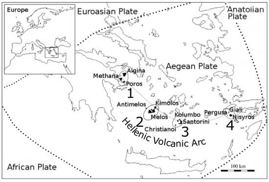
Figure 1.
The Hellenic Volcanic Arc: 1. Methana group, 2. Melos group, 3. Santorini group, and 4. Nisyros group.
One obvious approach used to correlate volcanic rocks and fingerprint ancient artifacts is to use the geochemistry of these rocks to identify their provenance. By studying the binary K2O versus SiO2 diagram [4] of the HVA compiled from 1500 data samples (Figure 2) [2], major overlaps of the data points can be seen. It is obvious that no discrimination between the volcanic regions of the HVA can be established based on this diagram.
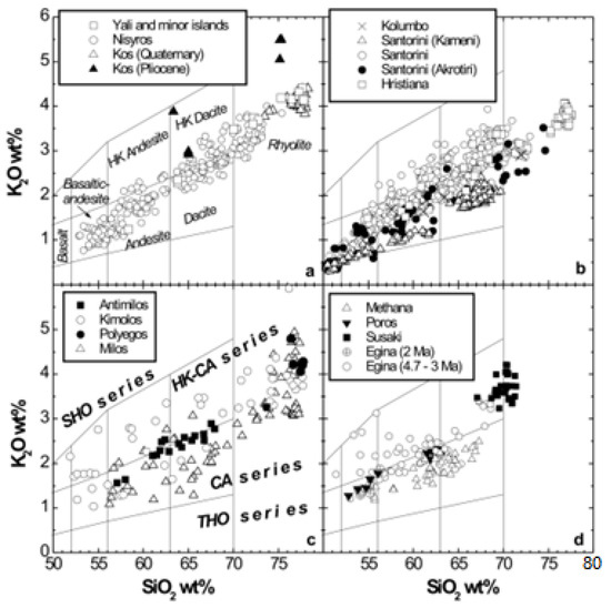
Figure 2.
K2O versus silica classification diagrams [4] for (a) Nisyros group (b) Santorini group (c) Melos group and (d) Methana group.
The diagram in Figure 2 is based on binary and ternary diagrams, known as discrimination diagrams, which were introduced in the 1970s to discriminate geotectonic settings based on the trace element [5] and major element [6] geochemical data of basalts and sandstones, respectively. The main geotectonic settings are the boundaries of either converging or diverging lithospheric plates where volcanic activity is observed, resulting in the formation of basalts, the most common rock formed by magma pouring out from volcanoes originating from the Earth’s mantle. Basalts can also be formed at hot spots far away from tectonic boundaries, which are known as Ocean Island Basalts (OIB). Given the small amount of data available and the limited areas under examination at the time, discrimination diagrams performed well and this is why they are still used and are continuously being evolved [7,8,9]. Since 1970, however, the amount of rock data acquired from all over the world has rapidly increased. Huge datasets containing information on the chemical analysis of rock samples have become openly available from databases such as GEOROCK [10] and PetDB [11]. These datasets have been used to prove that conventional discrimination diagrams are inaccurate in many cases [12,13] because of the overlap of the sample points, as is the case in the diagram in Figure 2.
Machine learning (ML) has been used in many fields of science to study the hidden patterns in large datasets [14]. After 2000, attempts have been made to use this technology to discriminate tectonic settings. The first successful attempt to discriminate tectonic settings using ML was made using Decision Trees (DT) in 2006 [15]. Ten years later, a Support Vector Machine (SVM) was tested on a dataset using the geochemical and isotopic data of basalts to discriminate tectonic settings [16]. One year later, SVM, Random Forest (RF), and Sparse Multinomial Regression (SMR) were compared using 20 elements and five isotopic ratios of basaltic rocks. The accuracy achieved was over 83% [17]. In 2019, chemical data derived from olivine, a major mineral found in basalts, were used to compare the accuracy of Logistic Regression (LR), Naïve Bayes (NB), RF, and Multi-Layer Perceptron (MLP) for discriminating tectonic settings [18]. The same group introduced a new method named SONFIS incorporating fuzzy logic [19]. The latest published work used the Logistic Regression Analysis (LRA) algorithm with the geochemical data of monazite, a mineral found in basalt rock [20]. In 2017, SVM was used to discriminate volcanic centers in Italy [21].
In this research, the aforementioned methodology used for discriminating tectonic settings was applied in order to evaluate its suitability for distinguishing volcanic regions belonging to one tectonic setting. This was accomplished by comparing the performance of 10 MLAs using six variations of the initial dataset retrieved from the GEOROCK databases. Only major elements were used, as usable trace element data were only available for 10% of the samples of the dataset. Finally a cloud-based application (CBA) was implemented using the best performing model with the ability to correlate a volcanic rock sample from the HVA with one of the four volcanic regions of the South Aegean, based on the geochemical composition of 10 major elements (SiO2, TiO2, Al2O3, Fe2O3T, CaO, MgO, MnO, K2O, Na2O, and P2O5). This application is publicly accessible at www.geology.gr (accessed on 6 September 2021).
2. Materials and Methods
2.1. Machine Learning Algorithms
The goal of ML is to construct a model for making predictions [22]. There are two essential parts to constructing a model: (1) the Machine Learning Algorithm (MLA) [23] and (2) the data. A wide variety of MLAs have been developed since the 1960s, and their improvement has never ceased. The choice of the best-performing algorithm is determined heuristically for a given problem. The best learning algorithm is considered to be the one that has low bias and accurately relates the input to the output values, achieving low variance, meaning that it can successfully predict the same result using different datasets. The latter is also called generalization. Ten MLAs, both linear and non-linear, were used in this study (Figure 3).
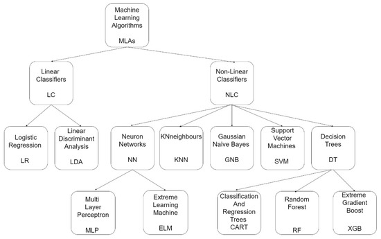
Figure 3.
Outline of the Machine Learning Algorithms used.
Of the linear algorithms, Logistic Regression (LR) [24] and Linear Discriminant Analysis (LDA) [25] were used. The non-linear algorithms tested were k-Nearest Neighbor (kNN) [26], Gaussian Naive Bayes (GNB) [27], and Support Vector Machine (SVM) [28]. Furthermore, Multi-Layer Perceptron (MLP) [29,30] and Extreme Learning Machine (ELM) [31,32] belonging to the Neural Network Group were evaluated. Finally, decision trees were tested, namely Classification and Regression Trees (CART) [33], Random Forest (RF) [34,35,36], and Extreme Gradient Boost (XGB) [37,38].
2.1.1. Logistic Regression
The LR algorithm [24] is an extension of the linear regression algorithm [39], where the goal is to find the ‘line of best fit’ in order to map the relationship between the dependent variable and the independent variables. The LR algorithm predicts whether something belongs to a class or not, i.e., if it is true or false. LR is mainly used for binary classification but can be extended for multiclass classification. In our case, Multinomial Logistic Regression was used.
2.1.2. Linear Discriminant Analysis
LDA is a supervised algorithm which reduces dimensionality. LDA is a two-class classifier but can be generalized for multi-class problems. The linear discriminants are the axes, which maximize the distances of multiple classes [25].
2.1.3. k-Nearest Neighbor
In the kNN classifier [26], the distances of the sample points are calculated from a random central point, and each data point is grouped according to this distance. It is regarded as one of the simplest MLAs. The k parameter indicates the number of points that will be taken into account. Larger values create high bias and should be avoided. Another parameter to be selected is the way the distance is computed. Some options are: (1) Euclidean distance, (2) Manhattan distance, and (3) Minkowski distance.
2.1.4. Gaussian Naïve Bayes
The GNB is a probabilistic non-parametric classifier and, as the name implies, is based on Bayes’ theorem [27].
2.1.5. Support Vector Machine
SVM is a supervised classification technique and was initially developed for binary classification problems. The main idea is that input vectors are mapped in a non-linear way to a very high-dimension feature space. A linear decision surface is constructed in this feature space. When a dataset consisting of three features is trained by an SVM, each point is plotted in the three-dimensional space. The algorithm’s goal is to classify the points by applying three planes. In the case of n features, the points are projected in an n-dimensional space, which cannot be visualized. The algorithm’s goal is to classify the objects by dividing the n-dimensional space with the use of what is known as hyperplanes. Predictions are achieved by projecting new points in these divisions [28].
2.1.6. Multi-Layer Perceptron
An MLP is a type of feedforward Artificial Neural Network (ANN). ANNs are based on the assumption that the way the human brain operates can be mimicked artificially by creating artificial neurons named perceptrons [30]. This is achieved by providing input and output data to the algorithm, which tries, by changing the weights of its neurons, to create a function that successfully maps the relationship between the input and the output data. In the case of the MLP, at least three layers are required: the input layer, the hidden layer, and the output layer. Each node is a neuron that uses a non-linear activation function. In this way, the MLP can classify separable non-linear data [29].
2.1.7. Extreme Learning Machine
ELMs are essentially neural networks with only one hidden layer. According to the original authors [32], this algorithm performs faster than MLPs with good generalization. In an ELM, the hidden nodes’ learning parameters, such as the input weight and biases, are randomly assigned and, according to the author, no tuning is needed. Furthermore, the output weights are determined by a simple inverse operation [31]. The only parameter tuned is the number of neurons in the hidden layer.
2.1.8. Classification and Regression Trees
When CART is used, classification of the samples is achieved by the binary partitioning of a feature [33]. It is not only the ease and robustness of construction that make CART a very attractive classifier. The big advantage is the possibility of interpreting the classification, which is either difficult or not possible at all with the aforementioned classifiers. Another advantage is the ability of classification trees to handle missing data. The disadvantage, however, is the overfitting problem. The tree created works well with the data used to create it but does not perform that well with new data. This is also called low bias–high variance. No parameters are set in this algorithm.
2.1.9. Random Forest
To deal with the overfitting problem of CART, the ensemble classifier RF was developed [35,36]. The main idea is to use many trees instead of one. The trees are built by using randomly selected subsets of the original data. The only constraint is that all the vectors must have the same dimensions. This is called bootstrapping. The results obtained from each tree are then put to a vote. The aggregate is the final result. This technique is known as bagging (from bootstrap aggregation) [34]. The split at each node is made by randomly selecting a subset of features. As the number of trees grows, better generalization is achieved. The parameters that can be set are: (1) the number of trees, (2) the number of features used to make the split at each node, and (3) the function used to measure the effectiveness of the split.
2.1.10. Extreme Gradient Boost
XGB is the latest classifier in the evolution of tree-based classifiers. It introduced tree gradient boosting [38]. Furthermore, XGB can handle sparse data [37]. According to the authors, XGB runs 10 times faster than other solutions.
2.2. Data Preparation
A collection of volcanic rock geochemical data, covering the active volcanic regions (4) of the HVA and most non-active pre-Pliocene volcanic regions (32) of Greece, was retrieved from the GEOROC database [10]. The initial dataset provided consists of 6229 entries containing 181 features. The first 41 features are descriptive and cover general information about the rock samples. Most notable is the year of publication of the rock sample data and the sampling location. Initially, data reduction was performed using the Python libraries Pandas [40] and Numpy [41] in nine sequential steps (Figure 4). In the first step, all rock sample entries published before 1985 [12] were deleted because analytical methods—the way the chemical composition was analyzed—prior to this year are considered unreliable. This resulted in a new data matrix with the dimensions of 5506 × 181. In the second step, 39 of the first 41 features were deleted. The ‘LOCATION’ feature was preserved, as it was essential for creating the classes in the eighth step. The ‘CITATION’ feature was used to select the validation data in the ninth step. In this way, the data matrix was reduced to 5506 × 142. The first feature represents the location and the second represents the scientific paper where the sample’s chemical composition was published, while the other 140 features contain the geochemical data of the rock samples. The chemical composition is expressed was the mass fraction (wt%) of the major elements, trace elements in parts per million (ppm) or parts per billion (ppb), and isotopes as ratios. In the third step, locations outside the research area were deleted, resulting in a 4153 × 142 data matrix.
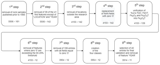
Figure 4.
Block diagram of the data preparation steps.
Moreover, in the initial dataset, many NAN fields were present, which could be computed by the MLAs; therefore, in the fourth step, these were replaced with zeroes and, consequently, no data matrix dimension change occurred.
The chemical compositions provided by GEOROC were determined using the XRF method. Depending on the methodology used, the iron oxides’ mass fraction (wt%) was provided either in FeO, FeOT, Fe2O3, or Fe2O3T. Thus, in the fifth step, to calculate the mass fraction uniformly, these four features were unified into one (Fe2O3T) through the following procedure: all oxides measured as FeOT were transformed to Fe2O3T by first multiplying the wt% of FeOT’s chemical composition by 1.1111. The chemical composition of FeO was multiplied by 1.1111 to obtain its chemical composition in Fe2O3, then, this value was added to the initial value of Fe2O3, resulting in the Fe2O3T. In this way, the table’s new dimensions were 4153 × 139.
In the sixth step, features where zeroes represented more than 65.29% (this value corresponds to the oxide P2O5) were deleted. This was necessary, as features beyond this threshold had zero values higher than 90%, making them useless for the training process of a ML model. This produced a 4153 × 12 data matrix. In the seventh stage, 199 entries had to be deleted as all 10 of their geochemical data fields were equal to zero. The emerging new data matrix’s dimensions were 3954 × 12. In the eighth step, the classes were prepared based on the four volcanic groups of the HVA [1,2]. Methana along with Aigina and Paros were labeled as Class 1. Melos together with Antimelos and Kimolos were labeled as Class 2. Santorini with Christianoi and Kolumbo were labeled as Class 3, and finally, Nisyros with Giali, and Pergoussa were labeled as Class 4.
In the final ninth step, 40 entries were randomly handpicked from the dataset to compile the validation dataset. This was done with the following constrains: 10 samples from each class, with each sample from a different publication and year. Furthermore, the ‘CITATION’ feature was removed, as it was no longer needed. This resulted in a 3914 × 11 matrix dimension for the final dataset.
Following data reduction, six datasets (All datasets are available upon request) were created. The initial dataset was labeled Dataset 1 and consisted of 3914 entries and 11 features. The first 10 features were the geochemical data of the major elements and the last was the class. A snapshot of Dataset 1, the initial dataset, is shown in Table 1. These 3914 data samples were used to plot SiO2 vs. K2O [42] (Figure 5) and SiO2 vs. Na2O + K2O [43] (Figure 6) to check if the four volcanic regions could be discriminated by the use of this bigger dataset. The diagrams show that this was not the case, as major overlapping of the sample points was present. In Dataset 2, the zeroes were replaced by the mean value. In Dataset 3, the zeroes were replaced by the median. Datasets 4–6 were created from Datasets 1–3 correspondingly by deleting the outliers. The outliers were removed by using the stats class of the Scipy library and the Numpy library. The number of entries of each class in every dataset is shown in Table 2. The basic statistic data of Datasets 1–6 are presented in Table 3, Table 4, Table 5, Table 6, Table 7 and Table 8. The histograms of Datasets 1–3 with outliers are depicted in Figure 7. The histograms of Datasets 4–6 with the outliers removed are depicted in Figure 8. The histogram of Dataset 5 shows the best distribution of the data.

Table 1.
Snapshot of Dataset 1.
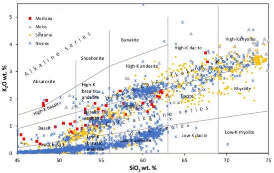
Figure 5.
K2O vs. SiO2 diagram.
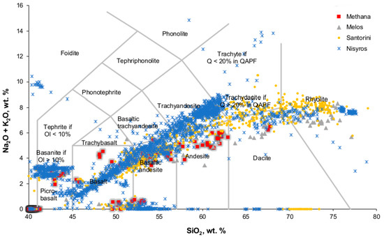
Figure 6.
Na2O + K2O vs. SiO2 diagram.
Table 2.
Classes and entries of Datasets 1–6.
Table 3.
Basic statistics of Dataset 1.
Table 4.
Basic statistics of Dataset 2.
Table 5.
Basic statistics of Dataset 3.
Table 6.
Basic statistics of Dataset 4.
Table 7.
Basic statistics of Dataset 5.
Table 8.
Basic statistics of Dataset 6.
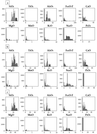
Figure 7.
Histograms of the datasets with outliers: (a) Dataset 1, (b) Dataset 2, and (c) Dataset 3.
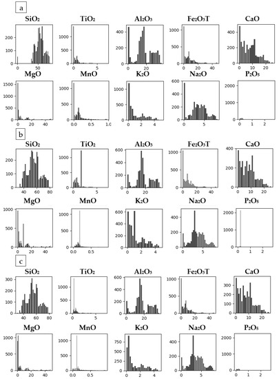
Figure 8.
Histograms of the datasets after outlier removal: (a) Dataset 4, (b) Dataset 5, and (c) Dataset 6.
2.3. Simulations
The training of the models was implemented using Python 3.8 (Guido van Rossum, The Hague, The Netherlands) [44] joint with Scikit-learn (David Cournapeau, Paris, France) [45], the xGboost wrapper for Scikit-learn(https://xgboost.readthedocs.io/, accessed on 30 June 2021) and elm.ELM Kernel (Augusto Almeida, Brazil). The goal was to create the most accurate model, with the smallest standard deviation and the least computing time, by using one out of the 10 MLAs and one of the six datasets. Training of the model was conducted on a Windows 10 System with an Intel Core 2 Quad Q8400 CPU and 8 GB of RAM. Tenfold cross-validation was applied (i.e., the original sample was randomly partitioned into 10 equal size subsamples). The datasets were split randomly into 70% training data and 30% testing data. In this way, the experiments were repeated 10 times by using 10 different versions of the dataset. Finally, three stages of testing and three improvement procedures were applied (Figure 9).
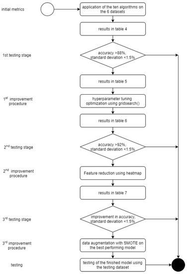
Figure 9.
Flowchart of the model’s development.
The initial metrics were computed by using the six datasets on the 10 algorithms with their default parameters.
The threshold values for the first testing stage were an accuracy of >88% and a standard deviation of <1.5%. In the following initial improvement procedure, a grid search was applied to the MLAs of the models passing the first testing stage to optimize the selected model’s algorithms.
The second testing stage had a threshold accuracy of >92% and the standard deviation remained at <1.5%. The models outperforming all the others were then put into the second improvement procedure, where feature reduction was applied using the results of a heatmap.
In the third testing stage, the goal was to improve accuracy by keeping the standard deviation of <1.50%. Following this, a confusion matrix [46] was compiled for the best-performing model. This revealed that a third improvement procedure was necessary to augment the data. Namely, the Synthetic Minority Over-sampling Technique (SMOTE) [47] was applied to the best-performing model’s dataset. Finally, the best-performing model was tested using the testing data, i.e., the 40 entries left out of the training and validation.
3. Results
The results of the first testing stage showed accuracy ranging from 48.39% (2.24% standard deviation, 2.01 s) for the model using GNB with Dataset 2 to 92.75% (1.36% standard deviation, 11.48 s) for the model using XGB with Dataset 5 (Table 9, Figure 10).
Table 9.
Testing results for the first testing stage (LR: Logistic Regression, LDA: Linear Discriminant Analysis, SVM: Support Vector Machine, KNN: K Nearest Neighbor, GNB: Gaussian Naïve Bayes, MLP: Multi-Layer Perceptron, ELM: Extreme Learning Machine, CART: Classification and Regression Trees, RF: Random Forest, XGB: xGBoost, std: standard deviation).
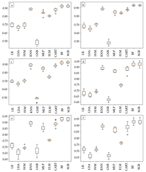
Figure 10.
Boxplots of the simulation results: (a) Dataset 1, (b) Dataset 2, (c) Dataset 3, (d) Dataset 4, (e) Dataset 5, and (f) Dataset 6.
Six models met the requirements of the first testing stage (>88% accuracy and <1.5% standard deviation). These were Model 1: kNN combined with Dataset 6 (88.58% accuracy, 1.08% standard deviation, 3.77 s); Model 2: RF with Dataset 3 (91.64% accuracy, 1.24% standard deviation, 10.39 s); Model 3: RF with Dataset 5 (92.73% accuracy, 1.46% standard deviation, 9.64 s); Model 4: RF with Dataset 6 (92.69% accuracy, 1.48% standard deviation, 9.05 s); model 5: XGB combined with Dataset 1 (91.57% accuracy, 1.34% standard deviation, 13.19 s); and Model 6: XGB combined with Dataset 5 (92.75% accuracy, 1.36% standard deviation, 11.48 s). All MLAs were used with their standard parameters (Table 10).
Table 10.
Best performing models (first testing stage).
The performance of a MLA can be optimized by changing a set of parameters. Each MLA has its own parameter that can be fine-tuned. The six models were improved in the first improvement procedure by using the gridsearch() function [45], which allows bulk testing of models on a selected set of parameters. This procedure is known as hyperparameter tuning. In the second testing stage (accuracy >92%, standard deviation <1.5%), only three models reached these stricter criteria, namely Model 3: RF with Dataset 5 (92.79% accuracy, 1.29% standard deviation, 16.13 s); Model 4: RF with Dataset 6 (92.75% accuracy, 1.35% standard deviation, 15.91 s); and Model 5: XGB combined with Dataset 5 (92.80% accuracy, 1.48% standard deviation, 18.97 s). A side effect of the improvement in accuracy was a rise in computational time during the training (Table 11).
Table 11.
Performance improvement of the models after hyperparameter tuning (first improvement procedure).
In the second improvement procedure, the best models from the second testing stage were analyzed to accomplish feature reduction. A heatmap was used to rank the features of Datasets 5 and 6 and further improve Models 3, 4, and 6. The features of Dataset 5 were reordered as follows: Al2O3, TiO2, CaO, P2O5, Na2O, MnO, SiO2, Fe2O3T, MgO, and K2O. The features of Dataset 6 were reordered as follows: Al2O3, CaO, Na2O, TiO2, MnO, P2O5, SiO2, Fe2O3T, K2O, and MgO. After using all the rearranged features, the three models showed minor improvements (Table 12). Model 6 achieved the best results. Rearranging the features resulted in an improvement in computational time. By removing features based on the aforementioned ranking, no increase in accuracy was achieved.
Table 12.
Performance improvement of the models after applying a heatmap (second testing stage, second improvement procedure).
In the third improvement procedure, a confusion matrix was created for Model 6 to evaluate the accuracy of each class (Figure 11a). The low prediction accuracy results of Melos can be explained if we take into account that an extremely imbalanced dataset was used: 132 entries for Methana, 104 for Melos, 906 for Santorini, and 2263 for Nisyros (Table 2).
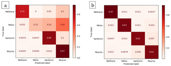
Figure 11.
Confusion matrix of (a) Model 6 and (b) Model 6 with the augmented Dataset 5—balanced 900.
For this reason, SMOTE was applied to augment Dataset5. One new dataset was created, labeled Dataset 5—balanced 900. The confusion matrix (Figure 11b) showed an improvement. The final model was devised by using the optimized XGB algorithm and Dataset 5—balanced 900 created by this imputation. Accuracy improved to 93.07% and the standard deviation was calculated as 1.21%.
This final model was tested with the 40 handpicked entries left out of the training and testing data. In this validation sample, 90% accuracy was achieved. The Methana class scored 100% and the Melos class scored 80%. One sample was misclassified as Santorini and one as Nisyros. The Santorini class scored 90%, with only one sample being misclassified as Melos. The Nisyros class scored 90%, one sample being misclassified as Santorini.
4. Discussion
The SiO2 vs. K2O diagram plotted in this study using 3914 data points showed that it is not possible to discriminate the tectonic regions by using this methodology. This is in accordance with the SiO2 vs. K2O diagrams of the HVA’s volcanic regions using 1500 data points in 2005 [1]. In order to classify the volcanic regions, the simulations showed that the best result was achieved by Model 6, which used the XGB classifier and a dataset where imputation was applied by replacing the zero values with the mean value and where the outliers were removed (Dataset 5). This final model performed at an accuracy of 92.75%. After hyperparameter tuning, feature rearrangement, and data augmentation had been applied, the accuracy reached 93.07%. This shows that this procedure can augment accuracy and should always be applied. It is notable to mention that Model 1, which used the kNN classifier with Dataset 6, performed at an accuracy of 91.26% with a very low computational cost of only 3.21 s. The final validation was conducted using the validation dataset consisting of 40 entries left out of the training and testing which resulted in an accuracy of 90%.
This study is in accordance with the positive results obtained from the Calabrian Volcanic Arc [21]. In this study, a similar dataset was used to discriminate the volcanic groups of Central Italy in the framework of tephrochronological studies using the SVM classifier. In this research, 98% accuracy was achieved.
The use of the model developed in the present study should not be used as a black box. Other means of examining the rock samples, such as mineralogy and the age of crystallization, must be taken into account to cross-validate the model’s results. The misclassification of four samples of the validation dataset shows that further improvement of the methodology described is necessary. This will be possible by retraining the selected classifier with new data which will emerge in the future.
5. Conclusions
The results of this research prove that the ML methodology used for discriminating tectonic environments can also be used to discriminate volcanic regions belonging to the same tectonic setting. In the case of the present study, four volcanic regions of the HVA producing IABs in a converging tectonic environment were successfully discriminated using the XGB classifier with an accuracy of 93.07% during training and 90% during validation.
The final model compiled was used for the implementation of a CBA [48] written in Python code and deployed in the flask framework. The CBA implemented in the framework of this study can be used as a valuable tool in the field of geology to classify volcanic rocks found in the Southern Aegean Sea in one of the four active volcanic regions of the HVA using 10 major elements. This will also be a useful tool for mapping of the HVA in the future. Furthermore, in geoarchaeology, the CBA can be used as a valuable tool for tracking the origin of artifacts found all over Greece, such as millstones and anchors made from volcanic rock dating from prehistory to antiquity, a procedure known as geochemical fingerprinting. The CBA is publicly accessible at www.geology.gr (accessed on 6 September 2021).
The authors’ future plans include applying this methodology for the two active volcanic arcs in the Mediterranean, namely the Hellenic Volcanic Arc in the Aegean Sea and the Calabrian Volcanic Arc in the Tyrrhenian Sea, as similar datasets are available in the GEOROC database. This would produce a tool for applying geochemical fingerprinting of ancient artifacts to a broader geographic region.
Author Contributions
Conceptualization, A.G.O. and G.A.P.; methodology, A.G.O. and G.A.P.; software, A.G.O.; validation, A.G.O. and G.A.P.; investigation, A.G.O.; writing—original draft preparation, A.G.O.; writing—review and editing, A.G.O. and G.A.P.; visualization, A.G.O.; supervision, G.A.P.; project administration, G.A.P. All authors have read and agreed to the published version of the manuscript.
Funding
This research received no external funding.
Institutional Review Board Statement
Not applicable.
Informed Consent Statement
Not applicable.
Data Availability Statement
The Geochemical Rock Database used in this study was retrieved from the Max Planck Institute for Chemistry, http://georoc.mpch-mainz.gwdg.de/georoc/ accessed on 30 June 2021.
Acknowledgments
We would like to pay our respects to all the individuals involved in collecting rock samples in the field, those in the laboratory producing the geochemical data, and, last but not least, the people responsible for GEOROC preparing the datasets and distributing them for free. This research would not have been possible without them. Moreover, we wish to express our gratitude to the geologists Katrivanos Manolis and Ntarlagiannis Nikos for reviewing the geological context of this paper. Finally, we would like to thank Michailidou Vasiliki for linguistic revision of the manuscript.
Conflicts of Interest
The authors declare no conflict of interest.
References
- Francalanci, L.; Vougioukalakis, G.E.; Perini, G.; Manetti, P. A West-East Traverse along the Magmatism of the South Aegean Volcanic Arc in the Light of Volcanological, Chemical and Isotope Data. Dev. Volcanol. Elsevier 2005, 7, 65–111. [Google Scholar] [CrossRef]
- Fytikas, M.; Innocenti, F.; Manetti, P.; Peccerillo, A.; Mazzuoli, R.; Villari, L. Tertiary to Quaternary Evolution of Volcanism in the Aegean Region. Geol. Soc. Lond. Spec. Publ. 1984, 17, 687–699. [Google Scholar] [CrossRef]
- Pe-Piper, G.; Piper, D.J.W. The South Aegean Active Volcanic Arc: Relationships between Magmatism and Tectonics. Dev. Volcanol. Elsevier 2005, 7, 113–133. [Google Scholar] [CrossRef]
- Peccerillo, A.; Taylor, S.R. Geochemistry of eocene calc-alkaline volcanic rocks from the Kastamonu area, Northern Turkey. Contr. Mineral. Petrol. 1976, 58, 63–81. [Google Scholar] [CrossRef]
- Pearce, J.A.; Cann, J.R. Tectonic Setting of Basic Volcanic Rocks Determined Using Trace Element Analyses. Earth Planet Sci. Lett. 1973, 19, 290–300. [Google Scholar] [CrossRef]
- Bhatia, M.R. Plate Tectonics and Geochemical Composition of Sandstone. J. Geol. 1983, 91, 611–627. [Google Scholar] [CrossRef]
- Snow, C.A. A Reevaluation of Tectonic Discrimination Diagrams and a New Probabilistic Approach Using Large Geochemical Databases: Moving beyond Binary and Ternary Plots. J. Geophys. Res. 1973, 111, B06206. [Google Scholar] [CrossRef] [Green Version]
- Vermeesch, P. Tectonic Discrimination Diagrams Revisited. Geochem. Geophys. Geosystems 2006, 7. [Google Scholar] [CrossRef]
- Zhang, Q.; Sun, W.; Zhao, Y.; Yuan, F.; Jiao, S.; Chen, W. New Discrimination Diagrams for Basalts Based on Big Data Research. Big Earth Data 2019, 3, 44–45. [Google Scholar] [CrossRef] [Green Version]
- Max Planck Institute for Chemistry. Geochemical Rock Database. Available online: http://georoc.mpch-mainz.gwdg.de/georoc/ (accessed on 29 June 2021).
- Lehnert, K.; Robinson, S. EarthChem. Available online: https://www.earthchem.org/petdb (accessed on 29 June 2021).
- Li, C.; Arndt, N.T.; Tang, Q.; Ripley, E.M. Trace Element Indiscrimination Diagrams. Lithos 2015, 232, 76–83. [Google Scholar] [CrossRef]
- Han, S.; Li, M.; Ren, Q.; Chengzhao, L. Intelligent Determination and Data Mining for Tectonic Settings of Basalts Based on Big Data Methods. Acta Petrol. Sin. 2018, 34, 3207–3216. [Google Scholar]
- Papakostas, G.A.; Diamantaras, K.I.; Palmieri, F.A. Emerging Trends in Machine Learning for Signal Processing. Comput. Intell. Neurosci. 2017, 2017, 1–2. [Google Scholar] [CrossRef] [PubMed] [Green Version]
- Vermeesch, P. Tectonic Discrimination of Basalts with Classification Trees. Geochim. Et Cosmochim. Acta 2006, 70, 1839–1848. [Google Scholar] [CrossRef]
- Petrelli, M.; Perugini, D. Solving Petrological Problems through Machine Learning: The Study Case of Tectonic Discrimination Using Geochemical and Isotopic Data. Contrib. Miner. Pet. 2016, 171, 81. [Google Scholar] [CrossRef] [Green Version]
- Ueki, K.; Hino, H.; Kuwatani, T. Geochemical Discrimination and Characteristics of Magmatic Tectonic Settings: A Machine-Learning-Based Approach. Geochem. Geophys. Geosyst. 2018, 19, 1327–1347. [Google Scholar] [CrossRef] [Green Version]
- Ren, Q.; Li, M.; Han, S. Tectonic Discrimination of Olivine in Basalt Using Data Mining Techniques Based on Major Elements: A Comparative Study from Multiple Perspectives. Big Earth Data 2019, 3, 8–25. [Google Scholar] [CrossRef] [Green Version]
- Ren, Q.; Li, M.; Han, S.; Zhang, Y.; Zhang, Q.; Shi, J. Basalt Tectonic Discrimination Using Combined Machine Learning Approach. Minerals 2019, 9, 376. [Google Scholar] [CrossRef] [Green Version]
- Itano, K.; Ueki, K.; Iizuka, T.; Kuwatani, T. Geochemical Discrimination of Monazite Source Rock Based on Machine Learning Techniques and Multinomial Logistic Regression Analysis. Geosciences 2020, 10, 63. [Google Scholar] [CrossRef] [Green Version]
- Petrelli, M.; Bizzarri, R.; Morgavi, D.; Baldanza, A.; Perugini, D. Combining Machine Learning Techniques, Microanalyses and Large Geochemical Datasets for Tephrochronological Studies in Complex Volcanic Areas: New Age Constraints for the Pleistocene Magmatism of Central Italy. Quat. Geochronol. 2017, 40, 33–44. [Google Scholar] [CrossRef] [Green Version]
- Jordan, M.J.; Mitchell, T.M. Machine learning: Trends, perspectives, and prospects. Science 2015, 349, 255–260. [Google Scholar] [CrossRef] [PubMed]
- Mitchell, T.M. Machine Learning, 1st ed.; McGraw-Hill Education: New York, NY, USA, 1997. [Google Scholar]
- Peng, C.-Y.J.; Lee, K.L.; Ingersoll, G.M. An Introduction to Logistic Regression Analysis and Reporting. J. Educ. Res. 2002, 96, 3–14. [Google Scholar] [CrossRef]
- Li, T.; Zhu, S.; Ogihara, M. Using Discriminant Analysis for Multi-Class Classification: An Experimental Investigation. Knowl. Inf. Syst. 2006, 10, 453–472. [Google Scholar] [CrossRef]
- Cover, T.; Hart, P. Nearest Neighbor Pattern Classification. IEEE Trans. Inform. Theory 1967, 13, 21–27. [Google Scholar] [CrossRef]
- John, G.H.; Langley, P. Estimating Continuous Distributions in Bayesian Classifiers. arXiv 2013, arXiv:1302.4964. [Google Scholar]
- Cortes, C.; Vapnik, V. Support-Vector Networks. Mach. Learn. 1995, 20, 273–297. [Google Scholar] [CrossRef]
- Collobert, R.; Bengio, S. Links between Perceptrons, MLPs and SVMs. In Proceedings of the Twenty-First international conference on Machine learning-ICML ’04, Banff, AB, Canada, 20 September 2004; ACM Press: Banff, AB, Canada, 2004; p. 23. [Google Scholar] [CrossRef] [Green Version]
- Minsky, M.; Papert, S. Perceptrons; M.I.T. Press: Oxford, UK, 1969. [Google Scholar]
- Ding, S.; Xu, X.; Nie, R. Extreme Learning Machine and Its Applications. Neural Comput. Appl. 2014, 25, 549–556. [Google Scholar] [CrossRef]
- Huang, G.-B.; Zhu, Q.-Y.; Siew, C.-K. Extreme Learning Machine: Theory and Applications. Neurocomputing 2006, 70, 489–501. [Google Scholar] [CrossRef]
- Breiman, L.; Friedman, J.H.; Olshen, R.A.; Stone, C.J. Classification And Regression Trees, 1st ed.; Routledge: Boca Raton, FL, USA, 2017. [Google Scholar] [CrossRef]
- Breiman, L. Bagging Predictors. Mach. Learn. 1996, 24, 123–140. [Google Scholar] [CrossRef] [Green Version]
- Breiman, L. Random Forests. Mach. Learn. 2001, 45, 5–32. [Google Scholar] [CrossRef] [Green Version]
- Tin Kam Ho. Random Decision Forests. In Proceedings of 3rd International Conference on Document Analysis and Recognition; Institute of Electrical and Electronics Engineers Computer Society Press: Montreal, QC, Canada, 1995; Volume 1, pp. 278–282. [Google Scholar] [CrossRef]
- Chen, T.; Guestrin, C. XGBoost: A Scalable Tree Boosting System. In Proceedings of the 22nd ACM SIGKDD International Conference on Knowledge Discovery and Data Mining; ACM: San Francisco, CA, USA, 2016; pp. 785–794. [Google Scholar] [CrossRef] [Green Version]
- Friedman, J.H. Greedy Function Approximation: A Gradient Boosting Machine. Ann. Statist. 2001, 29, 1189–1232. [Google Scholar] [CrossRef]
- Yan, X.; Su, X.G. Linear Regression Analysis: Theory and Computing; World Scientific Publishing Company: Singapore, 2009. [Google Scholar] [CrossRef]
- Mckinney, W. Data Structures for Statistical Computing in Python. In Proceedings of the 9th Python in Science Conference, Austin, TX, USA, 9–15 July 2010. [Google Scholar]
- van der Walt, S.; Colbert, S.C.; Varoquaux, G. The NumPy Array: A Structure for Efficient Numerical Computation. Comput. Sci. Eng. 2011, 13, 22–30. [Google Scholar] [CrossRef] [Green Version]
- Ewart, A. The Mineralogy and Petrology of Tertiary-Recent Orogenic Volcanic Rocks: With a Special Reference to the Andesitic-Basaltic Compositional Range. In Andesites: Orogenic Andesites and Related Rocks; Thorpe, R.S., Ed.; Wiley: Chichester, UK, 1982; pp. 25–95. [Google Scholar]
- Bas, M.J.L.; Maitre, R.W.L.; Streckeisen, A.; Zanettin, B.; IUGS Subcommission on the Systematics of Igneous Rocks. A Chemical Classification of Volcanic Rocks Based on the Total Alkali-Silica Diagram. J. Petrol. 1986, 27, 745–750. [Google Scholar] [CrossRef]
- Van Rossum, G.; Drake, F.L., Jr. Python Reference Manual; Centrum voor Wiskunde en Informatica: Amsterdam, The Netherlands, 1995. [Google Scholar]
- Pedregosa, F.; Varoquaux, G.; Gramfort, A.; Michel, V.; Thirion, B.; Grisel, O.; Blondel, M.; Müller, A.; Nothman, J.; Louppe, G.; et al. Scikit-Learn: Machine Learning in Python. arXiv 2018, arXiv:1201.0490. [Google Scholar]
- Kohavi, R.; Provost, F. Glossary of Terms. Mach. Learn. 1998, 30, 271–274. [Google Scholar] [CrossRef]
- Chawla, N.V.; Bowyer, K.W.; Hall, L.O.; Kegelmeyer, W.P. SMOTE: Synthetic Minority Over-Sampling Technique. J. Artif. Intel. Res. 2002, 16, 321–357. [Google Scholar] [CrossRef]
- Ouzounis, A. Geology in Greece. Available online: http://geology.gr/ (accessed on 6 September 2021).
Publisher’s Note: MDPI stays neutral with regard to jurisdictional claims in published maps and institutional affiliations. |
© 2021 by the authors. Licensee MDPI, Basel, Switzerland. This article is an open access article distributed under the terms and conditions of the Creative Commons Attribution (CC BY) license (https://creativecommons.org/licenses/by/4.0/).