Abstract
Even though additive manufacturing is receiving increasing interest from aerospace, automotive, and shipbuilding, the legacy approach using tessellated form representation and cross-section slice algorithm still has the essential limitation of its inaccuracy of geometrical information and volumetric losses of final outputs. This paper introduces an innovative method to represent multi-material and multi-directional layers defined in boundary-representation standard model and to process complex sliced layers without missing volumes by using the proposed squashing operation. Applications of the proposed method to a bending part, an internal structure, and an industrial moulding product show the assurance of building original shape without missing volume during the comparison with the legacy method. The results show that using boundary representation and te squashing algorithm in the geometric process of additive manufacturing is expected to improve the inaccuracy that was the barrier of applying additive process to various metal industries.
1. Introduction
Additive manufacturing (AM) has garnered considerable research interest over the last decade and is considered an upcoming production process that can be used to realise new practical manufacturing. This paper describes geometric processing to derive final sections utilised by an additive machine controller directly from a CAD model. There is a common assumption that the additive manufacturing process chain is well known, but there are a number of variables that are less well understood. The common view of the chain from CAD to part is:
- 1.
- CAD model
- 2.
- Approximation as STL (or maybe AMF)
- 3.
- Transfer to pre-processing software and correction, if necessary
- 4.
- Slicing and offsetting
- 5.
- Generating supports, if necessary, and tool paths
- 6.
- Slice transfer to additive machine
- 7.
- Part manufacture
This chain has been established based on practical observations made, not theoretical information. Before describing the modern, planned chain proposed by Bonnard [1], the normally assumed chain origins have been discussed.
AM machines and graphics computers, which are forerunners to graphics cards, were introduced at around the same time. To understand why the stereolithography (STL) format has been used for the communication of solid data, the technological development made during this period should be examined. During this period, two main techniques existed for representing solids: constructive solid geometry (CSG) and boundary representation (BRep). Although these two uses very different methods for representation, the CSG method generated a BRep model for graphics because direct graphics from CSG models proved to be too slow. So, the boundary of a solid, essentially the “skin” between the inside and outside of a solid model was a common factor. However, there was then no agreed format for communicating boundary data to applications. Another solid modeling method, the Octree method, was used for communicating volumetric data but eventually the skin of the object, communicating using triangles, gained dominance as a graphics communication format [2].
The idea of producing a real physical model as a visualisation tool may have encouraged the use of triangles, in the form of an STL file [3], as a means of communication for additive manufacturing. However, the STL format is, and always has been, a format for graphics, not for communicating solid information, which is what is needed for additive processes. For graphics purposes it is unimportant that the triangles are unconnected, but for additive processes it is critical that the triangles match and that the whole set is closed. In graphics the triangles are used to colour parts of the screen, so connectivity is unimportant and visual gaps only an annoyance. Nor is the shape of the triangle critical because the normal vector is given explicitly and does not need to be calculated from the facet vertex positions, so avoiding the problem of degeneracy. However, slicing triangles can lead to numerical problems if they are long and thin. In addition, faceting of surface models which may not be closed and separate faceting of faces in solid models leads to problems of mismatched facets, again not a problem for graphics but a major problem for additive manufacturing. Dissatisfaction with STL has long been apparent. In 1994 Carleberg [4] suggested using STEP [5] for shape communication. Kumar and Dutta [6] produced a survey of different formats. However, despite the problems of STL, its use has continued unabated. The new suggestion, AMF (Additive Manufacturing Format) [7] corrects some of the shortcomings, by adding material and colour information, but is still, essentially, a graphics format, unsuited for communicating solid model data.
In the meantime, since the original additive machines appeared for 3D printing of solids, the use case of additive manufacturing has changed. The traditional use case was 3D visualisation models and prototype manufacture additive processes. Additive processes, though, have moved into real manufacturing with moulds (rapid tooling) and, as processes improved, for manufacture of real parts, repaired parts, and re-furbished parts. Even though the use case has broadened, mass production is still a challenge to AM processes because of lack of accuracy and the physical realities of additive processes. Most additive parts with curved or sloping surfaces have a characteristic step-wise surface roughness because models are sliced to produce layer shapes that are extruded in a single direction. Post-processing operations, such as grinding processes, solvent immersion, and EDM (Electrical Discharge Machining) subtraction, improve the surface accuracy, but only when the parts are slightly larger than the required shape. This is not guaranteed in the normal chain because facet corners are on surfaces but edges may lie outside or inside the real shape. In addition, while the facetting is done relative to the surface, slicing is done in the build direction that does not take the surface normal vectors into consideration. This can lead to the realised object having missing volume in places, which creates problems for subsequent manufacturing. Finally, the data format used for AM processes is a tessellated model, which means increasing the size of the data, if accuracy needs to be high. A further complication of using a facetted representation for additive processes is that finishing processes use the exact shape for control, which means that it is necessary to have two models of the same part and that these models will not match.
Renan Bonnard performed an examination of BRep (boundary representation) based additive process at the Ecole Centrale de Nantes [1]. His work led to the development of the STEP-NC standard for additive processes, which defines a consistent format for additive processes as part of a manufacturing chain. The seamless representation of the consistent data format shows the advantages in term of advanced data model [8], the environmental impact analysis [8], hierarchical manufacturing structure [9]. The philosophy of STEP-NC is oriented to keep the identical quality of manufactured products even though the machine tool is changed to a different one until the end-of-life stage of product life cycle. As a demonstration of this concept, Um et al. [10] proved the advantage of using STEP-NC in AM processes as part of remanufacturing.
Through the whole product life cycle, additive manufacturing is widely utilised for more complex applications. This means that additive manufacturing is considered as one of a number of production processes in the whole supply chain. Hybrid manufacturing, which combines subtractive processes and additive processes, has appeared in commercial machine tools and requirements for mixed process planning are discussed by Newman et al. [11]. Various application industries, as well as typical manufacturing industry, utilise AM, as mentioned by Lee [12]. Advanced production technology, such as 4D printing, has also been launched [13]. These new applications also present the need for STEP-NC in additive manufacturing. Medical products, aircraft, racing cars and dental work are recent applications of additive manufacturing, but STEP-NC does not cover all additive manufacturing specialised operations and features [14,15].
This paper proposes a novel data representation based on STEP-NC and a new geometric procedure for producing slice geometry. This data representation also follows Part 17 which address the additive manufacturing standard of ISO 14649. In Section 2 the representation method of STEP-NC Part 17 is introduced. Section 3 describes new features and representation of AM features based on the STEP-NC representation. Slicing operations and a way to ensure that volume is added for post-processing by machine tools follows in Section 4. Section 5 explains the result of experiments with several shapes. In Section 6, the difference between the approach presented and conventional models is described, with a discussion of results in Section 7. Conclusions are given in Section 8.
2. Representation Method of STEP-NC Part 17
Even though legacy data formats have been developed, there is still the gap of satisfying the requirements of improving geometric processing. Software systems for additive process require high slice density, multi material data format, and fine slicing operations in order to produce accurate shape. the data formats which are used are investigated from STL [3] to STEP-NC [16] and AMF [7], recently established as an international standard. Then, in this section, the proposed advanced data representation format for additive manufacturing which is specific for multi-material processes is discussed.
2.1. Multi-Materials in Additive Manufacturing
Along with the advance of additive machine tools, multi-material representations are required for the upcoming CAD/CAM/CNC chain for additive manufacturing. To fulfil the demands, there are existing efforts to depict the complexity of free-form surface and internal structures. Multiple material additive manufacturing is reviewed by Vaezi et al. [17]. They also found inherent limitations for multiple material printing and addressed the necessity for hybrid systems. Kokkinis et al. [18] proposed another usage of additive processes to produce multiple-material and shape-changing objects manipulated by magnetic control. Pa et al. [19] also produced low-profile antennas with multi-material additive manufacturing. Ge et al. [20] established the concept of “4D printing” with tailorable shape memory polymers and emphasised the necessity for simulation models. Liu et al. [21] addressed the quality issues of multi-material surfaces for bonding. Gupta and Tandon [22] proposed the gradient representation of multiple material and multiple colour of additive process. The new STEP-NC part (ISO 14649-17) for additive processes has the freedom to use many representations from simple lines to NURBS surfaces. The collection of representations is the source of a new data format of additive process.
2.2. Evolution of Data Representation
A survey of data formats for layered manufacturing was carried out by Kumar and Dutta [6] in 1997. It has long been recognised that improving the accuracy of handling geometric data requires a new representation format, even though STL has been the de-facto format used for communicating shapes in additive manufacturing. It should be pointed out that there is no technical necessity ot use either STL or any other facetted format. Slicing of exact Boundary Representation models was developed at the end of the 1970s in the BUILD system, though not then for additive manufacturing. Other slicing algorithms were developed in the 1980s and slicing exact models is a function for engineering drawings in CAD systems. The suggestion by Carleberg [4] of using STEP when that became a standard for solid model data exchange was logical and realistic. Pratt et al. [23] examined the issue of the accuracy of the STL representation in rapid prototyping during data transfer through the CAD-CAM-CNC chain and emphasised the usage of the STEP representation. Hiller and Lipson proposed a new data format representing the geometry with a triangulation based express format called AMF (Additive Manufacturing Format) to improve the accuracy from a flat triangle representation [7]. As well as data representation, it is necessary to improve geometric operations such as scanning and printing direction to maintain seamless representation accuracy. Wang et al. [24] proposed an optimisation method for printing direction to improve surface quality. Mohammed et al. [25] suggested the use of additive manufacturing in the industry of prosthetic rehabilitation. This application consists of scanning to construct the geometry of the relevant body area, for them the face, design and finally AM to create the prosthesis.
2.3. Necessity of Exact Model in Additive Manufacturing
The last piece of work mentioned above illustrates a difference in the use case of additive manufacturing. For mechanical parts, there is usually an exact model available, created using a CAD system. For aesthetic design parts scanned from real shape for example, the ’model’ can be either an agglomeration of points through which to fit surfaces or a file in STL format. It can be argued that it is unnecessary to create exact surfaces and that the use of a set of triangles together with manual finishing based on human aesthetic judgment is more efficient for individual design parts.
Similar considerations can be made about industrial design parts with aesthetic forms. In mechanical parts where the exact geometry exists, conversion into a facetted form such as STL or AMF is inefficient. Geometric intersections are stable and available through commercial and open source kernel systems. They are more efficient than intersecting a lot of triangles and numerically more stable.
Another important consideration is the stage in which the geometric data are approximated. In the ideal case, all shape information passes seamlessly until the numerical controller of the AM. And numerical controller directly generates approximated curve paths in the last minute. On the other hand, using the approximated model in early design stage causes the accumulation of the error made by the series of geometric processes. The best case is to reach the accuracy of numerical controller by using an exact model for efficiency and accuracy.
The STEP-NC format, see Bonnard et al. [26] under standardisation by ISO TC184/SC1 /WG7 as ISO 14649-17, allows communication of an exact model for direct control. The format also allows post-processing, if required by the manufacturer, to either STL or AMF with parameters determined from user requirements. In addition, Bonnard et al. [27] described that the two formats STL and AMF are enablers for rapid evolution but not suitable for delicate manufacturing. The STEP-NC format is also more appropriate if manufacture is switched between machines with different characteristics. Since STEP-NC records what is commonly termed a micro process-plan it is also suitable for archiving where the process parameters are recorded explicitly. Utilizing the advantages of the STEP-NC formats, Zhao et al. [28] explained that richness of information is also appropriate for machine simulations. For further considerations, see Um et al. [10] which compares existing data representations with the STEP-NC data representation in an additive manufacturing process for re-manufacturing.
2.4. Calculation of Added Volume
The surface quality issue of approximation model is already discussed by Carleberg in terms of product modeling dimension for final production [4]. Generating added volume is the next target to be improved for high quality and robust output of additive process. Special treatment of slicing operations are also applied to increase the efficiency of handling complex geometry. This type of treatment does not exist in subtractive processes. Slicing methods have been developed to enhance the surface roughness and part strength of the final part. Overhang and undercut are serious problems disrupting the output quality. The slicing algorithm for a 5-axis table is discussed by Lee and Jee [29]. Physical weakness is addressed and a modified slicing algorithm was proposed by Steuben et al. [30]. In terms of the material usage, topological optimisation is applied to additive manufacturing to reduce the amount of support structures generated after an additive volume is created. Wu et al. [31] proposed an application based specific infill structure algorithm to optimise added/removed interior supporting structures. Changing the direction is also applied in Voronoi cell structure, see Wang et al. [24].
3. Data Representation
The question for legacy CAM software for additive processes is how the target objects should be designed. Using STEP-NC is a key way to derive exact slices to fit the final shape the designer wants. ISO 14649-17 is the standard of STEP-NC for additive processes and is integrated with the other ISO 14649 parts for hybrid process plans. The intention of this section is twofold. Firstly, the STEP-NC data format is introduced with comparison to voxelisation method. Secondly, gradient boundary representation generated by various source types is introduced to describe multiple material or multiple colour object. Finally, we discuss how to apply both features to the build-up phase.
3.1. STEP-NC Standards
Multiple materials structure and complex structures inside the product are also applications of additive manufacturing. The ways in which these shapes are expressed is broadly used in tessellation or in the Voxelisation method. Voxelisation methods generally make the data size larger depending on the shape complexity, as with point clouds. It also has the disadvantage of not having the high resolution of the original features once converted. BRep is a way of expressing complex shape accurately with smaller capacity compared with voxels or triangles, as well as direct inputs of the squash operation which can produce accurate and high-quality results.
In the case of STEP-NC, additive features present some ways of expressing BRep based representation. Figure 1 shows the data structure for STEP-NC additive manufacturing. Based on part 10 of the existing STEP-NC, the following definitions were made for AM following the definitions for milling and turning. First, the features used in STEP-NC are: am_compound_ feature representing multiple added features in compound information structure, am_gradient_feature allowing graded materials and colours produced by additive process, and am_heterogeneous_feature defined by a mathematical function adjusting heterogeneous materials and colours. The operations consist of: am_oned_operation which produces one filament to obtain the full geometry, and am_twod_operation defining the attributes of guiding geometry, thickness and normal vector.
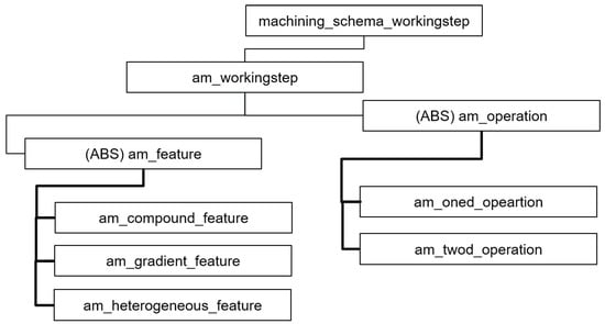
Figure 1.
The high-level structure of STEP-NC additive manufacturing.
3.2. Multi-Material Objects
The design methodology of multi-material objects is still unclear. This is not the objective of this study; however, insight into how the object was designed will be helpful for manufacturing. To address this gap, methods for defining multi-material objects have been developed.
For representing multi-material objects, explicit hard boundaries corresponding to graded materials can be employed, for which the material properties should be estimates, or voxel-based representations can be employed.
For explicit boundaries, the structure can be described using the boundary representation, BRep, with non-manifold internal boundaries. However, a few factors were considered. When the internal boundaries are not aligned with the build direction, which is unlikely, the squashing process defines overlapping areas where two materials are defined. The required alignment can be achieved using grading techniques or assigning material definition priorities such that one material will be chosen over another in the overlapping region. An interesting corollary to this is that holes can be defined as internal structures having an empty material. If the empty material has a higher priority than other materials, then this will force the hole to be open, although it may be larger than designed. In other cases, if the hole is oblique relative to the build direction, then the squashing process will tend to make the holes smaller. The problems of holes growing or diminishing in size are a side effect of the discrete nature of additive processes and must be considered by both designers and manufacturing planners.
Another method of representing multi-material objects is to provide a functional definition using material properties at a given point that can be calculated. An example of this is shown in Figure 2 using two surfaces as a guide for calculation.
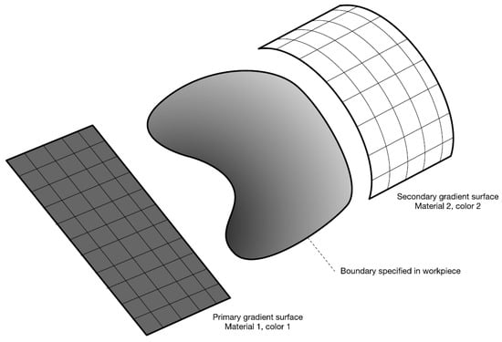
Figure 2.
Gradient surface of additive manufacturing.
Voxel-based methods use a cellular structure with explicit material properties assigned to each cell. There are known disadvantages of using voxel-based cellular representations. One is that the precision of the representation depends on the cell size, higher precision demanding more memory, so the representation is scale dependent. Another disadvantage is that the material properties of each cell are absolute, leading to hard internal boundaries rather than smooth grading. Voxel-based representations are, to some extent, attractive because of their simplicity and clear intention. However, it is not practical to expect users to define cell material properties explicitly for each cell. Instead, some sort of functional approach to material definition is realistic, but then this method could be defined in either BRep or the functional gradient approach.
For example, a BRep internal structure can use the ratio formulation [22] and requires a limited number of parameters to draw the material distribution.
In addition to the polynomial or linear functions, it is possible to use NURBS geometry to create internal patterns. Figure 3 shows a formulated model between two boundary curves having the relationship of gradient distribution from to . There is a correlation between each pair of vertices and . A NURBS formulation is applied along the line . In order to define the distribution, the input parameters are knot vectors, degrees, and control points to configure the distribution in multiple dimensions. NURBS also allows for multi-dimensional space in one-dimensional two-dimensional space, as well as more accurate representation of a given feature. In the slice operation, it is necessary to determine the colours for each slice and each path. Figure 4 depicts the colour allocation of each slice (a) and of each path (b).
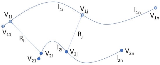
Figure 3.
The notation of gradient distribution of two boundary curves.
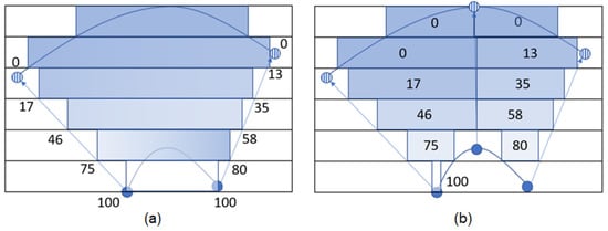
Figure 4.
Planar slicing results between two curves with gradient distribution: (a) each slice and (b) each path.
4. Slicing Operation
Approximation Slicing
The approximation depends on the distance of facets to the real surface rather than on the layered cross-sections. This means that it is likely that the corner points of planar sections do not actually lie on the real surface but on approximating facets inside or outside the real body. The result is a slight warping of the intended shape, possibly not noticeable to the eye but significant in terms of manufacturing precision. The larger the layer thickness compared to the feature details, the greater the problem.
The first step is to use the real geometry of the parts, rather than an approximation. This also leads to problems in obtaining the desired shape. The slicing problems are illustrated in Figure 5 and Figure 6. A common characteristic in both Figure 5 and Figure 6 is that the made shape lies inside the desired shape as the object expands and outside when the object is contracting, as indicated when comparing the red rings with the slices in both figures. In Figure 5, there is a representation of what might happen with a sphere. The right-hand side of the figure shows what might be the sections, the red ring indicates the shape intended. As with the approximated shape in Figure 5, the first section misses the body, since the intersection is at a single point. This means that the shape made is slightly higher than the desired shape. The yellow shape on the left represents a cross section through a sphere approximated by triangular facets.
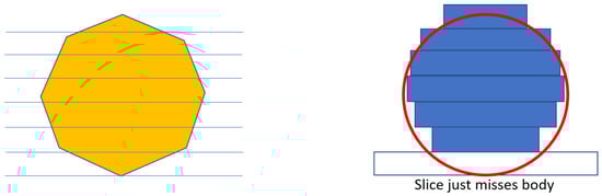
Figure 5.
Naive slicing from a facetted model.
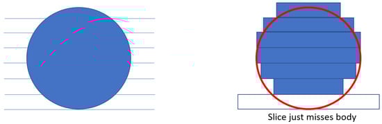
Figure 6.
Naive slicing.
It is also necessary to point out that the accuracy of surface approximation with facets is commonly controlled by a chord-height parameter. This controls the maximum allowable discrepancy from the real surface. However, this is in the direction of the local surface normal.Single directional additive manufacturing adds slices in an arbitrary direction irrespective of the real surface normal. This means that there is no guarantee that the solid created will respect the specified chord height tolerance. The desired slicing would be like the Figure 7.
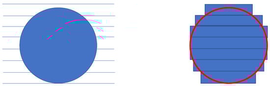
Figure 7.
Exact slicing with thick sliced.
This is simple geometric reasoning and fairly obvious. It is, however, important when considering additive manufacturing as part of a manufacturing process chain to make parts, where tolerance requirements are stricter than with visualisation. As indicated by the original use of additive processes, and the currently popular name of 3D printing, additive processes for visualisation have much lower requirements than for manufacturing and hence the need for a different control protocol.
For manufacturing, additive processes should be seen as part of a multi-process chain. Because of the nature of additive processes, surface finish and precision are lower and so, for critical parts of a piece, it is necessary to finish by machining. This implies that the additive part should be slightly larger than the desired part all over. To achieve this, the part footprint in each layer should be determined to, in turn, determine the slice profile. Instead of considering a single slice, the object is sliced below and above the section to be produced and this fat section is then squashed. The result is shown in Figure 7, with the material around the red-cross section; in effect, an intersection with a rectangular block of thickness equal to the layer thickness.
Another example of problems with naive slicing is shown in Figure 8. The desired object is shown at the top of Figure 8. The naive slicing, with a single slice profile is shown underneath. On the third row you have the result of additive with these simple slices. Depending on the angle of the slope, these elements may not even join and the whole sloping element would disappear. Even if they do join, the part thickness would diminish, possibly causing structural failure. With the thick sections you would obtain the object at the bottom which could then be finished by machining, if appropriate.
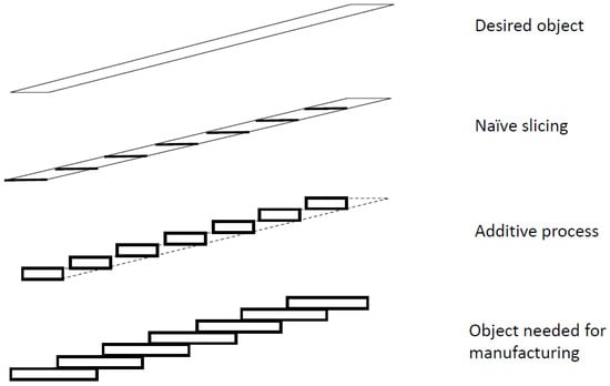
Figure 8.
Slice generation on sloping part.
The inaccuracy issues described above need to be resolved before machine tools start to build the final shape. Near-net-shape is required during geometric transformation to build the tool path for a numerical controller. Squashing is a way to extract Near-net-shape profiles and can be likened to making a pencil drawing around a fat section of the object laid on the floor. This is the silhouette of the fat slice viewed from the build direction. Each layer profile is projected onto the bottom plane and extruded along the identical direction with other slices. Squashing is similar to the common projection operation of solid kernel in terms of the range of Silhouette extraction from the cross-section of the designed shape.
5. Squashing Operation of Specialised Slicing
5.1. 2D Operation and Process Directions
Part 10 of STEP-NC, or ISO 14649-10, defines the boundary representation entities and other parts for different processes. Additive processes as well as milling process and turning process have process specific definitions in other parts. In Part 10, technological entities defining process parameters also cover some of those parameters needed for additive processes. Figure 9 illustrates a gradient that shows the distribution between two grid planes. By fitting parameters, NURBS can represent arbitrary distribution of internal structures captured by scanners or CT imaging. Different types of feature can also be created in the form of core profiles.
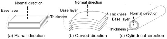
Figure 9.
2D operations of additive manufacturing.
Another way to define internal patterns as core profiles is to define the shape of slices according to the operation. Figure 9 shows three different regular slice geometries. The ’traditional’ slice geometry is a plane like Figure 9a. However, it is easy to imagine specialised machines to build curved or rotational parts, in which case different slicing geometries being useful. The most general is the cladding process which adds material to an existing object. In that case, it should be expected that a five axis machine needs to be used to apply material in general shapes. The shape of the ’slice’ and paths then become general and geometric forms such as NURBS are needed.
The operation is the same as the method to clean the core profile, but the usual use is planar slicing. However, depending on the shape, it may be efficient to use rotational or curved features. Profiles for these features are being organised at STEP-NC as Figure 9b,c.
5.2. Slicing Algorithm for Special Features
In the manufacturing process, the slicing algorithm is the most important operation to maintain accuracy of the AM process. The algorithm described here as shown in Algorithm 1 with notations on Table 1 uses a squashing operation to reduce the amount of gaps caused by the fluctuation of accumulated approximated sliced layers. This algorithm is able to keep fixed tolerance allowance and manage the empty space defined by the designer. Example of the algorithm applied on a single slice is described on Figure 10 and the overall specific procedure of the algorithm are shown in Figure 11.

Table 1.
Notations of the proposed squashing operation.
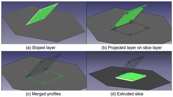
Figure 10.
Procedure of squashing operation on single slice: (a) select a shape to be squashed in the slice layer, (b) project all edges of a shape on the slice layer, (c) merge the edges and time the internal handing edges, and (d) extrude merged edges into a shell.
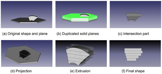
Figure 11.
Squashing Operation Process: (a) Original Shape and solid plane, (b) Duplicated solid planes by vertical direction, (c) Intersection part, (d) Projection, (e) Extrusion, (f) Final Shape.
Gradient interpolation is conducted during the slicing process. It does not use the approximated representation data format in the design phase but performs last minute modification to maximise accuracy in machine tool performance. The algorithm for building a squashing operation consists of five stages: (1) First, definition of the slicing plane which, with the layer thickness defines the slicing block. (2) Next, intersection using a Boolean operation between the slicing block and the desired object to calculate the actual slicing geometry of the layer. (3) Projection of all edges in the calculated slice along the slicing direction of each layer. Each projected edge becomes a portion of the slice boundary. The projected edges are then combined and the interior edges are removed to make the final profile. (4) Trimming of the profiles to remove dangling edges and ensure that the geometry is closed and manifold. Example of the non manifold cases are shown in Figure 12. (5) Extrusion of the projected profiles along the slicing direction.
| Algorithm 1: Squash partial section of manifold shape |
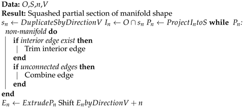 |
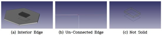
Figure 12.
Non-manifold cases caused by incorrect geometric processings: (a) The rectangular profile including an interior edge, (b) Two un-connected edges projected from the original shape, and (c) a failure for extruding broken profiles.
6. Case Studies
This section investigates the differences of representation methods in the design and manufacturing phases using STEP-NC additive manufacturing features. This section illustrates the differences and advantages of the proposed method which is defined in ISO 14649-17 [32] among STEP-NC standardisation methods. The method presented in this paper is applied to multi-material shapes and squash slices to increase the accuracy in the geometry definition process. In particular, this section shows data loss and changes in accuracy through manufacturing phases from computer-aided design tools and process planning tools, like CAM systems, in order to show the verification and comparison. In the design phase, the accuracy and data size of additive shapes are analysed and, in particular, representation methods for controlling distributions to multi-colour are compared. In the process planning phase, the accuracy of the geometric operation of slicing algorithm is investigated in terms of missing volume and additional volume.
The case study is performed with different shapes so that individual functions highlight effective characteristics:
- 1.
- Comparison of two shapes for the distribution of two materials
- 2.
- Comparison of the volume of missing and additional volume according to slicing in different directions for curved features
- 3.
- Example of slicing column geometry with cooling channels
The quantitative comparison of the proposed method above verifies the differences in function.
6.1. Gradient Distribution
NURBS was applied to two different 2D shapes in order to show the distribution of two colours. Figure 13 of two shapes shows the benefits are carried out of proposed methods. Examples are the front of a wardrobe and a curved beam to show the variety of AM process. These shapes are composed of different gradient colour changes from pink to blue. The top-left is the wardrobe coloured by simple distribution from top to bottom whereas top-right is coloured with the pink source coming from the top-right corner. The bottom-right shows a NURBS distribution with control points on curved beam while the bottom-left is the result of discretizing the cross-section of the beam shape. The representation of the NURBS distribution requires 5 × 5 control points, degree 2 in u and v, 2 knot vectors consisting of 9 real numbers. Discretizing is done after the CAM system loads a STEP-NC file. Thus, a discretised shape, like sampling number, polygon or voxel size, is not necessary for storing geometric data based on STEP-NC.
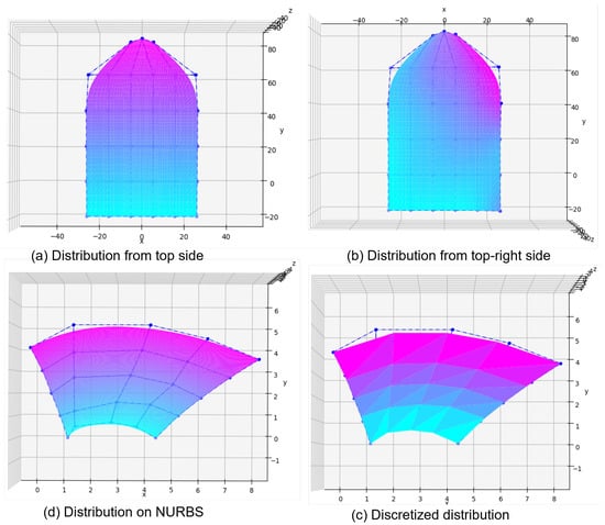
Figure 13.
Gradient distribution of NURBS function: (a) A tower shape including top-side gradient, (b) A tower shape including right top-side gradient, (c) A curved bean discretized gradient, (d) A curved beam including top-side gradient.
6.2. Squashing Operation for Curved Part
The goal of the second test problem is to show how different slice geometries affect the accuracy of the created object. In both cases the squashing algorithm is used to create slices to ensure that there is no missing material. For comparison, the traditional slicing process for the object is shown in Figure 14.
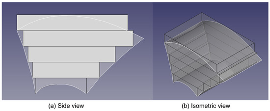
Figure 14.
A result of legacy slicing in side view (a) and isometric view (b).
The input geometry is a curved beam. The geometry of this model is shown in Figure 15a. The slicing algorithm was applied to each layer, with the result shown in Figure 15b. The slice lines due to intersection with the layer planes are shown in side view in Figure 15c. The object which would result is shown in side view in Figure 15d, with the target shape in darker grey and the layers as they would be in lighter grey.
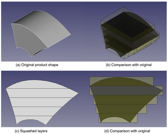
Figure 15.
A result of squashing operation with planar direction: (a) CAD file to be produced, (b) Transparent slices made by the proposed squashing algorithm, (c) The product shape split by slice boundaries, and (d) side of slice layer and the product shape.
Comparing Figure 14 with Figure 15d the difference between classic slicing (Figure 14) and thick slicing and squashing (Figure 15d) can be clearly seen. Except at the top, where the slice extends outside the object, the result material is inside the desired shape with traditional slicing whereas the desired shape is surrounded by deposited material with the slicing-and-squashing method.
The squashing operation is important because it prevents missing material volumes and is consistent in adding material compared with traditional slicing. The squashing operation achieves consistency by combining the top and bottom sections together with silhouette geometry to calculate the material ’footprint’ as the section profile. Tool path generation differentiates between two methods of offsetting each slice: direct offsetting and modified offsetting after each slice is squashed. The particular layers, such as bottom layer and top layer, seen in this comparison were chosen as they exhibit the highest missing volume of the slices. A comparison of the results produced by the legacy slicing operation is shown in Table 2. Table 2 describes that legacy slicing method could not describe the original shape perfectly since it looses the original shapes volume except for layer 5. The difference of volumes of the original shape and the outputs of both algorithms is shown in Table 3. As shown in Table 3, output of both algorithms(squash slicing, cylindrical slicing) has additional volume compared to the base(original shape), on the other hand legacy slicing algorithms has smaller volume which means it has lost its volume. For more specific result, Table 4 describes the volume of the each sliced layer and its summation on each different slicing algorithm.In Figure 15d, it is clear that the proposed algorithm produces an output that is close to original shape and does not show any missing volume.
Table 2.
Comparison of the volume of each layer.
Table 3.
Cylindrical slicing and squashing operation volume.
Table 4.
Comparison of Slicing method.
As well as missing volume, the gap resulting from slicing will be wider in the case of comparisons of shapes resulting from different file formats of STL and STEP-NC because slicing is performed on each profile that is extracted from the original shape represented by tessellated surface. The approaches to slice each layer reported recently are still aligned to direct slicing of tessellated shape even though Um and Stroud [10] already pointed out the issue of geometric accuracy. The challenge of achieving preservation of geometric accuracy imposes a significant hurdle to tool path generation of the additive process.
A related topic concerns the slicing with non-planar geometry. This is shown in Figure 16a,b. The base shape is shown with the regular slice geometry. Figure 16c,d shows the results. The left side of the figure shows a side view of the shape with the with resulting slices and the right-hand side of the figure shows what the resulting figure would look like. Circular slice geometry is used here to provide a simple comparison with planar geometry. Comparisons are given in Table 3.
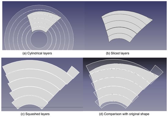
Figure 16.
A result of squashing operation with cylindrical direction: (a) the product shape and slice layers of cylindrical direction (b) the product shape split by slice boundaries, (c) slice layers made by the proposed squashing algorithm, and (d) the comparison of the product shape and slice layers.
Different slice geometry is important in processes such as cladding, which is used for repair of existing objects, turbine blades, and for remanufacturing. To repair the leading edge of a turbine blade it is necessary for the additive process nozzle to be moved along a complex curved path aligned with the surface normal where the repair is being carried out. In this case, the depths of the sliced layers are not necessarily uniform and vary along the slope. This kind of process requires better geometric reasoning for something like squashing operation and exact rather than approximated object geometry.
6.3. Squashing Operation of Empty Material
Additive manufacturing is widely thought of as capable of making any shape, however it is important to understand the limitations and implications. One of these concerns internal micro-structures such as holes, internal filaments or porous structures. Because of the discrete nature of the additive process there is a limit on the micro-structure size. Figure 17 shows how a sloping filament might be treated with traditional slicing so that either the filament does not unite or the thickness is less than planned. Another interesting question concerns small holes. An example of an object with a small hole is shown in Figure 18. With traditional slicing the sloping hole is blocked because the single slice is extruded upwards, not at an angle, so the starts and ends of the hole sections do not meet as shown in Figure 18a.
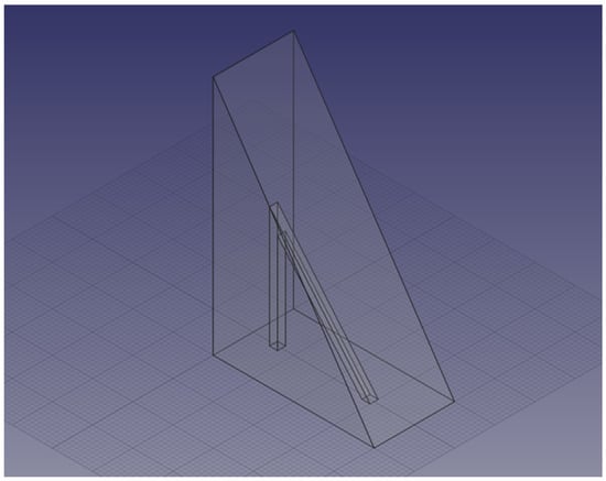
Figure 17.
Inner micro structure.
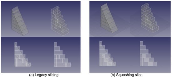
Figure 18.
Inner micro structures sliced by legacy operation (a) and squashing operation (b).
Normal squashing cannot help this problem because the material footprint would cover the hole. However, if the hole is defined as a core with empty material and if that material has a higher priority than the surrounding material, then the hole would consist of a set of connected cavities, as shown in Figure 18b. The top left of the figure depicts the object and the slice planes; top right, how the object would be cut; bottom left, the side view; and bottom right, the result with square cavities. However, this is not what the designer may expect.
6.4. Application to Industrial Shape
Figure 19 shows the application to a plastic product as the experiment of the proposed method. The squashed shape is produced by the proposed slicing algorithm. As the shown in the comparison of two sliced solid shapes. Left shape is smaller than right one due to the usage of legacy slicing. The results of toolpath generation identify the bottom paths are different from each other. The right squashed shape is a little bigger in order to avoid missing volume. And final outputs are also the evidence of how to keep the original volumes in leg part and bottom face.
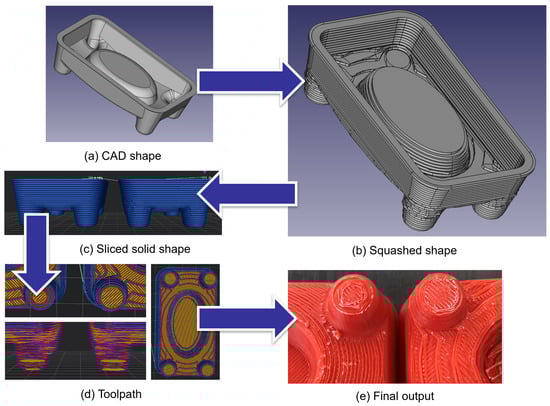
Figure 19.
Comparison with different slicing algorithms: The squashed sliced shape (b) made from CAD shape (a) is compared with the legacy sliced shape in terms of side views (c), tool-paths (d), and the final output (e).
7. Discussion
The results of the gradient distribution along the NURBS and squash slicing operation demonstrate that, in the design and manufacturing phases mentioned earlier, the case study considers multi-material-related cases. Further, the differences in features obtained following the squash operation were compared. The gradient case study demonstrates that the use of NURBS to define colour gives good results. It is more efficient in terms of storage space than both Voxelised and tessellated representations. The use of NURBS for multi-material definition has similar advantages. The second case study shows both the use of squashing to avoid missing volume in created shapes. This means that finishing processes such as milling or grinding can be used to remove extra material if necessary. The case study also shows the use of non-planar slicing techniques and quantifies the advantages for the object used. The use of non-planar slices is possible in some processes such as cladding. The third case study demonstrates the need for handling micro-holes in a special way using void material definitions. Through the comparison with the legacy method of the data representation and the slicing algorithm, the improvement in data size reduction, slicing accuracy, and inner structure are shown in Table 2, Table 3 and Table 4.
8. Conclusions
The representation based on the STEP-NC uses standardised and accurate CAD model to improve not only the information accuracy of data representation information but also the accuracy of tool-path generation. To this end, in this paper, various shape expressions and squashing algorithms were proposed and are proved as a solution to build complete shapes without any missing volume in several counterpart case examples. In the case of an industrial plastic products, the proposed method builds the shape sufficiently covered with the CAD model, compared to the legacy method, and does not cause a problem of volumetric loss. The hybrid process, including subtractive and additive processes, is a manufacturing method for producing the final form until post-processing in a single configuration. In a future work, it is necessary to use the proposed geometry algorithm in subtraction post-processing, such as milling or grinding, to remove the additional volumes made by squashed-slice algorithm. And the extension to post-processing is expected to improve the interoperability and machining quality in additive manufacturing.
Author Contributions
Author Contributions: Conceptualization, J.U., I.A.S.; investigation, J.U.; data curation, J.P., J.U.; writing—original draft preparation, I.A.S., J.U. and J.P.; writing—review and editing, I.A.S., J.U. All authors have read and agreed to the published version of the manuscript.
Funding
This work was supported by the National Research Foundation of Korea (NRF) grant funded by the Korea government (MEST) (No. NRF-2019R1G1A1100471) and KEIT (Korea Evaluation Institude of Industrial Technology) Korea Government(MOTIE: Ministry of Trade Industry and Energy) (No. 20016343).
Conflicts of Interest
Authors declared no potential conflict of interest with respect to the research, authorship, and/or publication of this article.
References
- Bonnard, R. Proposition de Chaine Numerique Pour la Fabrication Additive. Ph.D. Thesis, Ecole Centrale de Nantes (ECN), Nantes, France, 2010. [Google Scholar]
- Siraskar, N.; Paul, R.; Anand, S. Adaptive slicing in additive manufacturing process using a modified boundary octree data structure. J. Manuf. Sci. Eng. 2015, 137, 011007. [Google Scholar] [CrossRef]
- Roscoe, L.E. Stereolithography interface specification. Am.-3D Syst. Inc. 1988, 27, 10. [Google Scholar]
- Carleberg, P. Product model driven direct manufacturing. In Proceedings of the International Solid Freeform Fabrication Symposium, Austin, TX, USA, 8–10 August 1994. [Google Scholar]
- Industrial Automation Systems and Integration—Product Data Representation and Exchange—AP242 Managed Model Based 3D Engineering; Standard ISO 10303-242; International Standard Organization: Geneva, Switzerland, 2014.
- Kumar, V.; Dutta, D. An assessment of data formats for layered manufacturing. Adv. Eng. Softw. 1997, 28, 151–164. [Google Scholar] [CrossRef]
- Hiller, J.D.; Lipson, H. STL 2.0: A proposal for a universal multi-material additive manufacturing file format. In Proceedings of the Solid Freeform Fabrication Symposium, Ithaca, NY, USA, 3–5 August 2009; Volume 3, pp. 266–278. [Google Scholar]
- Le Bourhis, F.; Kerbrat, O.; Hascoet, J.Y.; Mognol, P. Sustainable manufacturing: Evaluation and modeling of environmental impacts in additive manufacturing. Int. J. Adv. Manuf. Technol. 2013, 69, 1927–1939. [Google Scholar] [CrossRef] [Green Version]
- Bonnard, R.; Hascoët, J.Y.; Mognol, P.; Zancul, E.; Alvares, A.J. Hierarchical object-oriented model (HOOM) for additive manufacturing digital thread. J. Manuf. Syst. 2019, 50, 36–52. [Google Scholar] [CrossRef]
- Um, J.Y.; Rauch, M.; Hascoet, J.Y.; Stroud, I. STEP-NC compliant process planning of additive manufacturing: Remanufacturing. Int. J. Adv. Manuf. Technol. 2017, 88, 1215–1230. [Google Scholar] [CrossRef]
- Newman, S.; Zhu, Z.; Dhokia, V.; Shokrani, A. Process planning for additive and subtractive manufacturing technologies. CIRP Ann. 2015, 64, 467–470. [Google Scholar] [CrossRef]
- Lee, B.N.; Pei, E.; Um, J. An overview of information technology standardization activities related to additive manufacturing. Prog. Addit. Manuf. 2019, 4, 345–354. [Google Scholar] [CrossRef]
- Pei, E.; Loh, G.H. Technological considerations for 4D printing: An overview. Prog. Addit. Manuf. 2018, 3, 95–107. [Google Scholar] [CrossRef] [Green Version]
- Flynn, J.M.; Shokrani, A.; Newman, S.T.; Dhokia, V. Hybrid additive and subtractive machine tools–Research and industrial developments. Int. J. Mach. Tools Manuf. 2016, 101, 79–101. [Google Scholar] [CrossRef] [Green Version]
- Zhu, Z.; Dhokia, V.G.; Nassehi, A.; Newman, S.T. A review of hybrid manufacturing processes–state of the art and future perspectives. Int. J. Comput. Integr. Manuf. 2013, 26, 596–615. [Google Scholar] [CrossRef] [Green Version]
- International Organization for Standardization. Industrial Automation Systems and Integration—Physical Device Control—Data Model for Computerized Numerical Controllers—Part 17: Process Data for Additive Manufacturing Processes; Standard ISO 14649-17; International Organization for Standardization: Geneva, Switzerland, 2016. [Google Scholar]
- Vaezi, M.; Chianrabutra, S.; Mellor, B.; Yang, S. Multiple material additive manufacturing—Part 1: A review: This review paper covers a decade of research on multiple material additive manufacturing technologies which can produce complex geometry parts with different materials. Virtual Phys. Prototyp. 2013, 8, 19–50. [Google Scholar] [CrossRef]
- Kokkinis, D.; Schaffner, M.; Studart, A.R. Multimaterial magnetically assisted 3D printing of composite materials. Nat. Commun. 2015, 6, 1–10. [Google Scholar] [CrossRef] [Green Version]
- Pa, P.; Larimore, Z.; Parsons, P.; Mirotznik, M. Multi-material additive manufacturing of embedded low-profile antennas. Electron. Lett. 2015, 51, 1561–1562. [Google Scholar] [CrossRef]
- Ge, Q.; Sakhaei, A.H.; Lee, H.; Dunn, C.K.; Fang, N.X.; Dunn, M.L. Multimaterial 4D printing with tailorable shape memory polymers. Sci. Rep. 2016, 6, 31110. [Google Scholar] [CrossRef] [Green Version]
- Liu, Z.H.; Zhang, D.Q.; Sing, S.L.; Chua, C.K.; Loh, L.E. Interfacial characterization of SLM parts in multi-material processing: Metallurgical diffusion between 316 L stainless steel and C18400 copper alloy. Mater. Charact. 2014, 94, 116–125. [Google Scholar] [CrossRef]
- Gupta, V.; Tandon, P. Heterogeneous object modeling with material convolution surfaces. Comput.-Aided Des. 2015, 62, 236–247. [Google Scholar] [CrossRef]
- Pratt, M.J.; Bhatt, A.D.; Dutta, D.; Lyons, K.W.; Patil, L.; Sriram, R.D. Progress towards an international standard for data transfer in rapid prototyping and layered manufacturing. Comput.-Aided Des. 2002, 34, 1111–1121. [Google Scholar] [CrossRef]
- Wang, W.M.; Zanni, C.; Kobbelt, L. Improved surface quality in 3D printing by optimizing the printing direction. Virtual Phys. Prototyp. 2016, 35, 59–70. [Google Scholar] [CrossRef]
- Mohammed, M.; Tatineni, J.; Cadd, B.; Peart, P.; Gibson, I. Applications of 3D topography scanning and multi-material additive manufacturing for facial prosthesis development and production. In Proceedings of the 27th Annual International Solid Freeform Fabrication Symposium, Austin, TX, USA, 8–10 August 2016; pp. 1695–1707. [Google Scholar]
- Bonnard, R.; Hascoet, J.Y.; Mognol, P.; Stroud, I. STEP-NC digital thread for additive manufacturing: Data model, implementation and validation. Int. J. Comput. Integr. Manuf. 2018, 31, 1141–1160. [Google Scholar] [CrossRef]
- Bonnard, R.; Hascoet, J.Y.; Mognol, P. Data model for additive manufacturing digital thread: State of the art and perspectives. Int. J. Comput. Integr. Manuf. 2019, 32, 1170–1191. [Google Scholar] [CrossRef]
- Zhao, G.; Cao, X.; Xiao, W.; Liu, Q.; Jun, M.B.G. STEP-NC feature-oriented high-efficient CNC machining simulation. Int. J. Adv. Manuf. Technol. 2020, 106, 2363–2375. [Google Scholar] [CrossRef]
- Lee, K.; Jee, H. Slicing algorithms for multi-axis 3-D metal printing of overhangs. J. Mech. Sci. Technol. 2015, 29, 5139–5144. [Google Scholar] [CrossRef]
- Steuben, J.C.; Iliopoulos, A.P.; Michopoulos, J.G. Implicit slicing for functionally tailored additive manufacturing. Comput.-Aided Des. 2016, 77, 107–119. [Google Scholar] [CrossRef]
- Wu, J.; Wang, C.C.; Zhang, X.; Westermann, R. Self-supporting rhombic infill structures for additive manufacturing. Comput.-Aided Deisgn 2016, 80, 32–42. [Google Scholar] [CrossRef]
- International Organization for Standardization. Industrial Automation Systems and Integration—Physical Device Control—Data Model for Computerized Numerical Controllers—Part 17: Process Data for Additive Manufacturing; Standard ISO/FDIS 14649-17; International Organization for Standardization: Geneva, Switzerland, 2019. [Google Scholar]
Publisher’s Note: MDPI stays neutral with regard to jurisdictional claims in published maps and institutional affiliations. |
© 2021 by the authors. Licensee MDPI, Basel, Switzerland. This article is an open access article distributed under the terms and conditions of the Creative Commons Attribution (CC BY) license (https://creativecommons.org/licenses/by/4.0/).