Design and Motion Simulation of an Underwater Glider in the Vertical Plane

Abstract

Net buoyancy, as the main power source for the motion of an underwater glider, is affected by the pump or bladder that the glider adopts to change its buoyancy force in water. In this study, a new underwater glider that can dive to a depth of 400 m at a cruising speed of 2 knots, which is faster than conventional underwater gliders and is less affected by sea currents, is investigated. The UG resisting 400 m pressure on the buoyancy engine and achieving 2 knots’ speed was designed and constructed. For this UG, its steady-state attitude was studied according to the variance of the buoyancy center and the center of gravity with the buoyancy engine influenced by the displacement of the movable mass block. In motion simulation of the UG, the attitude of the UG under different displacement conditions was simulated in Simulink according to the displacements of the piston and the movable mass block. To validate the simulation performance, a UG was constructed and experiments were conducted. The simulation and experimental results were compared to show the reliability of the simulation results under limited conditions.

1. Introduction

Unmanned underwater vehicles, such as remotely operated vehicles (ROVs) and autonomous underwater vehicles (AUVs), have been used to investigate the underwater terrain or work under the water. Sometimes, small ROVs are used to identify unidentified targets [1,2]. However, the working range of ROVs is limited such that AUVs have been used for a wide range of areas. Autonomous underwater gliders, one kind of AUV, have been developed and investigated for decades as devices that enable long-range underwater detection and reconnaissance [3]. An underwater glider (UG) is a new type of underwater monitoring platform [4]; it comprises a pair of fixed wings assembled on both sides of the fuselage, as well as a controllable rudder to realize the change in motion direction. A variable-volume buoyancy engine causes changes in its own buoyancy; when the buoyancy force is less than the gravity force, the engine sinks in the water, and when the gravity force is less than the buoyancy force, it floats in the water. During the sinking and surfacing motions, the fixed wing is subjected to hydrodynamic force, which generates a horizontal force to drive the glider forward. The gliding pitch angle of the glider is changed by adjusting the position of the internal adjustable mass block in the body through the internal structure. A heat engine was investigated for use as an energy source of the buoyancy engine of a SLOCUM glider; additionally, the linear movement of the battery pack for controlling the glider’s pitching motion underwater was analyzed [5]. The mass configuration of a buoyancy-driven underwater glider was decomposed and defined, and the glider motion was established and investigated using MATLAB [6]. System identification was conducted to investigate the ballast system of a USM underwater glider to understand the pumping rate as the input of the system and the corresponding net buoyancy of the ballast system. The estimation was performed using various models available in the MATLAB System Identification Toolbox, in which the ARMAX model was selected as the best model to represent the system and to obtain the transfer function. In addition, the glider depth and pitching angle were monitored [7]. The hydrodynamic performance of the underwater glider was analyzed using FLUENT software to provide a reference basis for the ideal design of each section of the body, and the motion in the vertical plane of the underwater glider was analyzed. The variation curves of the angle of attack (AOA) and attitude angle were obtained for different net buoyancies, different center of gravity displacements, and different speeds [8]. The motion of the glider in the vertical plane was simulated and analyzed to derive a relationship between the pitch angle of the glider and each of the axial displacements of the slider and the net buoyancy [9].

For the underwater glider, under the premise of satisfying the performance, the structure should be designed as compact as possible in order to reduce the manufacturing cost, and the shape should be streamlined to reduce the resistance in an underwater operation so as to reduce the energy loss during the operation and to extend the mission time.

In this paper, a new UG resisting 400 m pressure on the buoyancy engine and achieving 2 knots’ speed was designed and constructed, and the related piston cylinder-type buoyancy engine and an internal mass block were studied. For the design of the UG, the net buoyancy and the movable range of the movable mass block were studied, and after determining the net buoyancy, the mass of the movable mass block could be indirectly determined. Based on the UG design, the parameters of the buoyancy engine and the movable mass were obtained.

In the glider motion simulation, the displacement of the piston and movable mass block were used as input conditions, which allowed a more visual representation of the effect of different displacements on the gliding parameters. Therefore, in this study, the main parameters of glider motion in the vertical plane, such as AOA, pitch angle, and glide angle, were analyzed and compared for different displacement conditions of the piston and the movable mass block; through the comparison of the gliding parameters, it was found that maintaining the consistency of the piston and movable mass block motion could lead to the best control performance of the glider during attitude transition.

2. UG Design

To achieve better mechanical properties for resisting seawater pressure and to facilitate fabrication, the shape of the underwater glider was designed by applying MYRING hull profile equations [10]. The MYRING hull profile is illustrated in Figure 1.

The head and stern sections are expressed as shown in Equations (1)–(3):

$$r_{\mathrm{head}}\left(x\right)=\frac{1}{2}d{\left[1-{\left(\frac{x-a}{a}\right)}^2\right]}^{\frac{1}{n}},0\le x\le a$$

(1)

$$r_{\mathrm{mid}}\left(x\right)=\frac{1}{2}d,a\le x\le a+b$$

(2)

$$\begin{array}{c}{r}_{\mathrm{stern}}\left(x\right)=\frac{1}{2}d-\left(\frac{3d}{2c^2}-\frac{\tan \delta }{c}\right){\left(x-a-b\right)}^2+\left(\frac{d}{c^3}-\frac{\tan \delta }{c^2}\right){\left(x-a-b\right)}^3,\\ a+b\le x\le a+b+c\end{array}$$

(3)

Here, $d$ represents the body diameter, $a$ represents the head length, $n$ can be used to determine the shape of the head section, $c$ represents the length of the stern section, and $\theta$ represents the tail wrap angle, which determines the shape of the stern. The greater the angle of $\delta$, the smoother is the shape change at the stern. The parameters of the MYRING hull profile equations in this study were as follows: $a$ = 280 mm, $b$ = 1530 mm, $c$ = 400 mm, $d$ = 260 mm, $n$ = 2, and $\tan \delta$ = 0.8.

Net buoyancy is the main driving force for the motion of an underwater glider, and it determines the performance and reliability of the glider. The underwater glider changes its buoyancy by drawing and discharging water through a built-in pump. When the net buoyancy is positive, the glider floats upward, and when the net buoyancy is negative, the glider moves downward. Furthermore, the glider is subject to hydrodynamic forces from water when moving underwater. The force analysis of the glider during stable gliding is presented in Figure 2.

The drag force can be expressed by

$$D=\frac{1}{2}\rho C_D{A}_D{V}^2$$

(4)

Here, $\rho$ is the density of the fluid, $C_D$ the drag coefficient of the glider, $A_D$ the cross-sectional area of the glider, and $V$ the gliding speed. During steady gliding in the water, the force will maintain balance on the glider; therefore, the net buoyancy $\mathsf{\Delta }B$ and hydrodynamic drag force D are correlated as follows:

$$D=\mathsf{\Delta }Bsin\mathsf{\zeta }$$

(5)

where $\mathsf{\zeta }$ is the gliding angle. Combining Equations (4) and (5), the net buoyancy is expressed as

$$\mathsf{\Delta }B=\frac{1}{2sin\mathsf{\zeta }}\rho C_D{A}_D{V}^2$$

(6)

The net buoyancy of the UG is expressed as

$$\mathsf{\Delta }B=m_{0}g=\rho V_{b}g$$

(7)

Here, $V_b$ is the volume of drainage of the buoyancy engine, and Equations (6) and (7) are merged to obtain the equation for the displacement of the buoyancy engine of the UG, which occurs as the gliding angle is 35° [11].

$$V_b=\frac{1}{2gsin\mathsf{\zeta }}{C}_D{A}_D{V}_{max}^2$$

(8)

Based on the design specifications, an underwater glider that can reach a maximum path speed of 2 knots was designed. Ji et al. [11] present a similar underwater glider with a diameter of 0.22 m, whose total drag coefficient is 0.2629. The water volume was obtained using the equations above. Considering the internal space of the waterproof housing and the compactness of the structure, the inner diameter of the cylinder of the buoyancy engine was set to 0.15 m. From the known conditions, the displacement of the piston can be calculated to be approximately 74.3 mm when the glider reaches the maximum speed. Taking into account the error in the theoretical calculation and the difference in the hydrodynamic drag coefficient, the effective stroke of the piston was set to 220 mm.

SolidWorks was used to construct a three-dimensional model of the underwater glider and to calculate the maximum displacement mass and center of gravity of the glider. Subsequently, an assembly model of the glider was constructed based on the center of gravity as the origin of the coordinates. The buoyancy of the glider $m_B$ at this moment can be obtained as follows:

$$m_B=M_B-m_b$$

(9)

Here, $M_B$ and $m_b$ present the maximum buoyancy and ballast water, separately.

In this study, the piston assembly was regarded as a movable mass block, and when the piston and movable mass were displaced, the center of gravity of the glider system changed accordingly. The underwater glider was regarded as a rigid body motion system composed of several masses, including the movable mass ($\overline{m}$), piston assembly ($m_p$), and stationary mass ($m_s$), which include the mass of the hull and the fixed wings. An illustration of the glider mass is shown in Figure 3.

The glider mass can be expressed as follows:

$$m=\overline{m}+m_p+m_s$$

(10)

If the glider is suspended in water, then the position of the movable mass is adjusted such that the glider is in horizontal suspension equilibrium in water. Subsequently, the net buoyancy of the glider is changed via the water absorption or drainage of the piston to drive the glider down or up, and the water absorption mass of the piston can be expressed as

$$m_0=u_0{d}_{p1}=\rho \pi r^2{d}_{p1}$$

(11)

Here, $r$ represents the inner radius of the buoyant cylinder and $d_{p1}$ represents the displacement of the piston (the direction of water absorption is positive). The position of the buoyancy center ($r_{CB}$) is calculated as follows:

$$r_{CB}=-m_b{r}_b/m_B$$

(12)

Here, $r_b$ is the position of ballast water in the body coordinate.

The terms $r_{\overline{m}}$, $r_p$, $r_b$, and $r_s$ in Figure 3 represent the position vectors of the movable mass, piston assembly, ballast water, and stationary mass to the origin of the body frame, respectively. The center of the glider mass is expressed as follows:

$$r_{CG}=\left(\overline{m}{r}_{\overline{m}}+{\mathrm{m}}_p{r}_p+{\mathrm{m}}_s{r}_s\right)/m$$

(13)

Because the movable mass and the piston can only move along the longitudinal axis of the glider, the x-axis dimension changes in the body coordinate system, the z-axis dimension is fixed, and the stationary mass is fixed in the body. Hence, the equation for the center of gravity of the glider can be derived. When the glider is suspended horizontally in water, the mass position of each mass block in the x-axis direction of the body coordinate are recorded as the initial positions of balance of $r_{\overline{m}i1}$, $r_{pi1}$, $r_{bi1}$,and $r_{si1}$. The details of the parameters are shown in

Table 1. Parameters of the glider (fresh water).

Term	Value	Description
$M_B$	79.99	Maximum buoyancy of glider (kg)
$m$	78.24	Mass of glider (kg)
$\overline{m}$	9.48	Mass of movable mass (kg)
${\mathrm{r}}_{\overline{m}i1}$	0.5463	Initial position of movable mass along x-axis (equilibrium) (m)
${\mathrm{r}}_{\overline{m}3}$	0.0397	Initial position of movable mass along z-axis (equilibrium) (m)
$m_p$	1.4840	Mass of piston assembly (kg)
${\mathrm{r}}_{pi1}$	0.1607	Initial position of piston along x-axis (equilibrium) (m)
${\mathrm{r}}_{p3}$	0.0287	Initial position of piston along z-axis (equilibrium) (m)
$m_s$	67.27	Mass of static equilibrium (kg)
${\mathrm{r}}_{si1}$	−0.0805	Initial position of static mass along x-axis (equilibrium) (m)
${\mathrm{r}}_{s3}$	0.0053	Initial position of static mass along z-axis (equilibrium) (m)
${\mathrm{m}}_{bi}$	1.75	Initial mass of ballast in neutral state (kg)
${\mathrm{r}}_{bi1}$	−0.0019	Initial position of ballast water along x-axis (equilibrium) (m)
${\mathrm{r}}_{b3}$	0.0287	Initial position of ballast mass along z-axis (equilibrium) (m)

below.

The mass center displacement of the movable mass, piston assembly, and ballast water are represented by $d_{\overline{m}}$, $d_p$, and $d_b$, respectively (the positive direction of the x-axis is recorded as a positive value).

$$r_{\overline{m}}=r_{\overline{m}i}+d_{\overline{m}}$$

(14)

$$r_p=r_{pi}+d_p$$

(15)

$$r_b=r_{bi}+d_b$$

(16)

$$d_b=\frac{1}{2}{d}_p$$

(17)

When the piston moves, the mass of ballast water in the buoyant cylinder after the suspension state changes accordingly, as follows:

$$m_b=m_{bi}+m_0$$

(18)

Subsequently, Equation (13) can be rewritten as

$$r_{CG}=\left(\overline{m}{d}_{\overline{m}}+{ \mathrm{m}}_p{d}_p+{ \mathrm{m}}_s{r}_s\right)/m$$

(19)

The relative position of the center of gravity to the center of buoyancy of the glider in different states can be deduced as follows:

$$r_r=r_{CG}-r_{CB}$$

(20)

Because only the motion of the glider in the vertical plane is analyzed in this study, the recovery moment of the glider is expressed as

$${\mathsf{\tau }}_{hs2}=mg\left({\mathrm{r}}_{rx}cos\theta +{\mathrm{r}}_{rz}sin\theta \right)$$

(21)

Here, the ${\mathrm{r}}_{rx}$ and ${\mathrm{r}}_{rz}$ present the position of center of gravity in x- and z-axes in the body coordinate, respectively.

3. Mathematical Model

To facilitate the study and analysis of the six degrees-of-freedom motion of the marine vessel, two different reference coordinate systems [12] were established: the Earth-fixed reference coordinate system (E-XYZ) and the body reference coordinate system (O-xyz). The Earth-fixed reference coordinate system uses any point at sea level and sets the floating center position of the underwater glider as the origin of the body reference coordinate system. The motion reference coordinates are shown in Figure 4.

The transformation matrix from the body-fixed frame O-xyz to the Earth-fixed frame E-XYZ is as follows:

$$R=\left[\begin{array}{ccc}\cos \psi \cos \theta & -\sin \psi \cos \varphi +\cos \psi \sin \theta \sin \varphi & \sin \psi \sin \varphi +\cos \psi \cos \varphi \sin \theta \\ \sin \psi \cos \theta & \cos \psi \cos \varphi +\sin \varphi \sin \theta \sin \psi & -\cos \psi \sin \varphi +\sin \theta \sin \psi \cos \varphi \\ -\sin \theta & \cos \theta \sin \varphi & \cos \theta \cos \varphi \end{array}\right]$$

(22)

The position of the glider $b={\left(x,y,z\right)}^T$ is the vector from the origin of the earth reference frame to the origin of the body-fixed frame. The linear motion velocities and angular velocities of the glider are expressed as $v={\left(v_1,v_2,v_3\right)}^T$ and $={\left({\mathsf{\omega }}_1,{\mathsf{\omega }}_2,{\mathsf{\omega }}_3\right)}^T$, respectively. For a vector $x={\left(x_1,x_2,x_3\right)}^T$, the skew-symmetric matrix is expressed as follows [13]:

$$\widehat{x}=\left[\begin{array}{ccc}0& -x_3& x_2\\ x_3& 0& -x_1\\ -x_2& x_1& 0\end{array}\right]$$

(23)

For any vector $y={\left(y_1,y_2,y_3\right)}^T$, the vector product of x and y is expressed as

$$\widehat{x}\mathit{y}=x\times y$$

(24)

Subsequently, the kinematics of a glider can be written as

$$\dot{R}=R\widehat{\omega }$$

(25)

$$\dot{b}=Rv$$

(26)

Let $P_E$ and ${\pi }_{\mathit{E}}$ represent the total linear momentum and angular momentum of the UG in the Earth-fixed reference coordinate, respectively; $P_{\overline{m},E}$ and $P_{\mathrm{P},E}$ represent the total momentum of the movable mass and piston in the Earth-fixed coordinate, respectively [13].

$${\dot{P}}_E={\displaystyle \sum }_{\mathit{i}=1}^{\mathit{I}}{f}_{\mathit{e}\mathit{x}\mathit{t},\mathit{i}}$$

(27)

$${\dot{\pi }}_E={\displaystyle \sum }_{\mathit{i}=1}^{\mathit{I}}\left(x_{\mathit{i}}\times f_{\mathit{e}\mathit{x}\mathit{t},\mathit{i}}\right)+{\displaystyle \sum }_{\mathit{j}=1}^{\mathit{J}}{\tau }_{\mathit{e}\mathit{x}\mathit{t},\mathit{j}}$$

(28)

$${\dot{P}}_{\overline{m},E}=\overline{m}\mathrm{g}k+{\displaystyle \sum }_{\mathit{k}=1}^{\mathit{K}}{f}_{int,\overline{m}}$$

(29)

$${\dot{P}}_{p,E}=m_p\mathrm{g}k+{\displaystyle \sum }_{\mathit{k}=1}^{\mathit{K}}{f}_{int,m_p}$$

(30)

Here, $\mathit{k}$ is a unit vector point in the direction of gravity, ${\mathit{f}}_{\mathit{e}\mathit{x}\mathit{t},\mathit{i}}$ the external force exerting on the glider system, and ${\mathbf{\tau }}_{\mathit{e}\mathit{x}\mathit{t},\mathit{j}}$ the external torque applied to the system. Vector ${\mathit{x}}_{\mathit{i}}$ applies the point of application of the external force with respect to Earth’s reference frame. The force ${\mathit{f}}_{int,\overline{m}}$ exerts on the movable mass from the glider body, and ${\mathit{f}}_{int,m_p}$ is the force applied from the glider body onto the piston.

Let $P$ represent the total linear momentum of the glider–fluid system expressed in the body-fixed reference frame. Let $\Pi$ be the total angular momentum of the origin of the body coordinate. Let $P_{\overline{m}}$ represent the momentum of the moving mass and $P_p$ the momentum of the pistons in the body frame.

$$P_E=RP$$

(31)

$${\pi }_E =R\Pi +b\times P_E$$

(32)

$$P_{\overline{m},E}=R{P}_{\overline{m}}$$

(33)

$$P_{p,E}=R{P}_p$$

(34)

Combining Equations (25) and (26), the derivatives on both sides of the equations above can be calculated as follows:

$${\dot{P}}_E=R\left(\dot{P}+\widehat{\mathbf{\omega }}P\right)$$

(35)

$${\dot{\pi }}_E =R\left(\dot{\Pi }+\widehat{\mathbf{\omega }}\Pi \right)+Rv\times P_E+b\times {\dot{P}}_E$$

(36)

$${\dot{P}}_{\overline{m},E}=R\left(\dot{P_{\overline{m}}}+\widehat{\mathbf{\omega }}{P}_{\overline{m}}\right)$$

(37)

$${\dot{P}}_{p,E}=R\left(\dot{P_p}+\widehat{\mathbf{\omega }}{P}_p\right)$$

(38)

The following dynamics equations are obtained in the body frame:

$$\dot{P}=P\times \omega +{\mathit{R}}^{\mathit{T}}{\displaystyle \sum }_{\mathit{i}=1}^{\mathit{I}}{\mathit{f}}_{\mathit{e}\mathit{x}\mathit{t},\mathit{i}}$$

(39)

$$\dot{\Pi }=\Pi \times \omega +\mathit{P}\times v+{\mathit{R}}^{\mathit{T}}{\displaystyle \sum }_{\mathit{i}=1}^{\mathit{I}}\left(\left({\mathit{x}}_{\mathit{i}}-\mathit{b}\right)\times {\mathit{f}}_{\mathit{e}\mathit{x}\mathit{t},\mathit{i}}\right)+{\mathit{R}}^{\mathit{T}}{\displaystyle \sum }_{\mathit{j}=1}^{\mathit{J}}{\mathbf{\tau }}_{\mathit{e}\mathit{x}\mathit{t},\mathit{j}}$$

(40)

$${\dot{P}}_{\overline{m}}=P_{\overline{m}}\times \omega +\overline{m}\mathrm{g}\mathit{k}+{\mathit{R}}^{\mathit{T}}{\displaystyle \sum }_{\mathit{k}=1}^{\mathit{K}}{\mathit{f}}_{int,\overline{m}}$$

(41)

$${\dot{P}}_p=P_p\times \omega +m_p\mathrm{g}\mathit{k}+{\mathit{R}}^{\mathit{T}}{\displaystyle \sum }_{\mathit{k}=1}^{\mathit{K}}{\mathit{f}}_{int,p}$$

(42)

Here, ${\mathit{R}}^{\mathit{T}}{\displaystyle \sum }_{\mathit{k}=1}^{\mathit{K}}{\mathit{f}}_{int,\overline{m}}$ is the internal force exerted on the movable mass in the body-fixed frame. Let

$${\dot{P}}_{\overline{m}}=u_{\overline{m}}=P_{\overline{m}}\times \omega +\overline{m}\mathrm{g}\mathit{k}+{\mathit{R}}^{\mathit{T}}{\displaystyle \sum }_{\mathit{k}=1}^{\mathit{K}}{\mathit{f}}_{int,\overline{m}}$$

(43)

$${\dot{P}}_p=u_p=P_p\times \omega +m_p\mathrm{g}\mathit{k}+{\mathit{R}}^{\mathit{T}}{\displaystyle \sum }_{\mathit{k}=1}^{\mathit{K}}{\mathit{f}}_{int,p}$$

(44)

The total glider–fluid kinetic energy is calculated, and the kinetic energy of the movable mass, piston, ballast mass, and static mass are expressed as follows:

$${\mathrm{T}}_s=\frac{1}{2}{\left(\begin{array}{c}v\\ \mathbf{\omega }\end{array}\right)}^T\left(\begin{array}{cc}{m}_s{\mathit{I}}_{3\times 3}& -m_s{\widehat{\mathit{r}}}_s\\ m_s{\widehat{\mathit{r}}}_s& {\mathit{J}}_s\end{array}\right)\left(\begin{array}{c}v\\ \mathbf{\omega }\end{array}\right)$$

(45)

$${\mathrm{T}}_{\overline{m}}=\frac{1}{2}{\left(\begin{array}{c}v\\ \mathbf{\omega }\\ {\dot{\mathit{r}}}_{\overline{m}}\end{array}\right)}^T\left(\begin{array}{ccc}\overline{m}{\mathit{I}}_{3\times 3}& \overline{m}{\widehat{\mathit{r}}}_m& \overline{m}{\mathit{I}}_{3\times 3}\\ \overline{m}{\widehat{\mathit{r}}}_m& -\overline{m}{\widehat{\mathit{r}}}_m{\widehat{\mathit{r}}}_m& \overline{m}{\widehat{\mathit{r}}}_m\\ \overline{m}{\mathit{I}}_{3\times 3}& \overline{m}{\widehat{\mathit{r}}}_m& \overline{m}{\mathit{I}}_{3\times 3}\end{array}\right)\left(\begin{array}{c}v\\ \mathbf{\omega }\\ {\dot{\mathit{r}}}_{\overline{m}}\end{array}\right)$$

(46)

$${\mathrm{T}}_p=\frac{1}{2}{\left(\begin{array}{c}v\\ \mathbf{\omega }\\ {\dot{\mathit{r}}}_p\end{array}\right)}^T\left(\begin{array}{ccc}{m}_p{\mathit{I}}_{3\times 3}& m_p{\widehat{\mathit{r}}}_p& m_p{\mathit{I}}_{3\times 3}\\ m_p{\widehat{\mathit{r}}}_p& -m_p{\widehat{\mathit{r}}}_p{\widehat{\mathit{r}}}_p& m_p{\widehat{\mathit{r}}}_p\\ m_p{\mathit{I}}_{3\times 3}& m_p{\widehat{\mathit{r}}}_p& m_p{I}_{3\times 3}\end{array}\right)\left(\begin{array}{c}v\\ \mathbf{\omega }\\ {\dot{\mathit{r}}}_p\end{array}\right)$$

(47)

The kinetic energy of a rigid body immersed in an ideal fluid can be expressed as follows:

$${\mathrm{T}}_f= \frac{1}{2}{\left(\begin{array}{c}v\\ \mathbf{\omega }\end{array}\right)}^T\left(\begin{array}{cc}{M}_f& D^T{}_f\\ D_f& J_f\end{array}\right)\left(\begin{array}{c}v\\ \omega \end{array}\right)$$

(48)

Here, $M_f$ is the added mass matrix, $J_f$ is the added inertia matrix, and $D_f$ is the added cross term. These matrices are determined by the body shape and the fluid density.

The total glider–fluid kinetic energy is expressed as

$$\mathrm{T} ={\mathrm{T}}_s+{\mathrm{T}}_{\overline{m}}+{\mathrm{T}}_p+{\mathrm{T}}_f$$

(49)

The rotational kinetic energy of a rigid body around the axis of rotation is expressed as

$${\mathrm{T}}_{rot}=\frac{1}{2}{\left(\begin{array}{c}v\\ \begin{array}{c}\omega \\ {\dot{r}}_{\overline{m}}\end{array}\\ {\dot{r}}_p\end{array}\right)}^{T}I\left(\begin{array}{c}v\\ \begin{array}{c}\omega \\ {\dot{\mathit{r}}}_{\overline{m}}\end{array}\\ {\dot{\mathit{r}}}_p\end{array}\right)$$

(50)

Here, the inertia of the total system is expressed as

$$I=\left(\begin{array}{cccc}{m}_s{\mathit{I}}_{3\times 3}+\overline{m}{\mathit{I}}_{3\times 3}+m_p{\mathit{I}}_{3\times 3}+{\mathit{M}}_f& -\overline{m}{\widehat{\mathit{r}}}_m-m{\widehat{\mathit{r}}}_{m_p}+{\mathit{D}}_f^T& \overline{m}{\mathit{I}}_{3\times 3}& m_p{\mathit{I}}_{3\times 3}\\ \overline{m}{\widehat{\mathit{r}}}_m+m_p{\widehat{\mathit{r}}}_{m_p}+{\mathit{D}}_f& {\mathit{J}}_s-\overline{m}{\widehat{\mathit{r}}}_m{\widehat{\mathit{r}}}_m-m_p{\widehat{\mathit{r}}}_{m_p}{\widehat{\mathit{r}}}_{m_p}+{\mathit{J}}_f& \overline{m}{\widehat{\mathit{r}}}_m& m_p{\widehat{\mathit{r}}}_{m_p}\\ \overline{m}{\mathit{I}}_{3\times 3}& -\overline{m}{\widehat{\mathit{r}}}_m& \overline{m}{\mathit{I}}_{3\times 3}& \mathbf{0}\\ m_p{\mathit{I}}_{3\times 3}& -m_p{\widehat{\mathit{r}}}_{m_p}& \mathbf{0}& m_p{\mathit{I}}_{3\times 3}\end{array}\right)$$

(51)

Subsequently, $P$, $\Pi$, $P_{\overline{m}}$, and $P_p$ can be calculated as follows:

$$\begin{gathered} P=\frac{\partial \mathit{T}}{\partial \mathrm{v}}=\left(m_s{\mathit{I}}_{3\times 3}+{\mathit{M}}_f\right)\mathit{v}+{\mathit{D}}^T{}_f\mathbf{\omega }+\overline{m}\left(\mathit{v}+\mathbf{\omega }\times {\mathit{r}}_{\overline{m}}+{\dot{\mathit{r}}}_{\overline{m}}\right) \\ +m_p\left(\mathit{v}+\mathbf{\omega }\times {\mathit{r}}_p+{\dot{\mathit{r}}}_p\right) \end{gathered}$$

(52)

$$\begin{array}{c}\Pi =\frac{\partial T}{\partial \omega }={\mathit{D}}^T\mathit{v}+\left({\mathit{J}}_s+{\mathit{J}}_f\right)\mathbf{\omega }+\overline{m}{\widehat{\mathit{r}}}_m\left(\mathit{v}+\mathbf{\omega }\times {\mathit{r}}_{\overline{m}}+{\dot{\mathit{r}}}_{\overline{m}}\right)\\ +m_p{\widehat{\mathit{r}}}_p\left(\mathit{v}+\mathbf{\omega }\times {\mathit{r}}_p+{\dot{\mathit{r}}}_p\right)\end{array}$$

(53)

$$P_{\overline{m}}=\overline{m}\left(\mathit{v}+\mathbf{\omega }\times r_{\overline{m}}+{\dot{\mathit{r}}}_{\overline{m}}\right)$$

(54)

$$P_p=m_p\left(\mathit{v}+\mathbf{\omega }\times {\mathit{r}}_p+{\dot{\mathit{r}}}_p\right)$$

(55)

The design of this glider can be regarded as symmetric about three planes for calculation convenience, where ${\mathit{M}}_f$ and ${\mathit{J}}_f$ are diagonal matrices and ${\mathit{D}}_f=\mathbf{0}$. Let ${\mathit{M}}_f=\mathrm{diag}\left(\begin{array}{ccc}{m}_{f1}& m_{f2}& m_{f3}\end{array}\right)$ and ${\mathit{J}}_f=\mathrm{diag}\left(\begin{array}{ccc}{J}_{f1}& J_{f2}& J_{f3}\end{array}\right)$.

$$\mathit{M}=m_s{\mathit{I}}_{3\times 3}+{\mathit{M}}_f=\left(\begin{array}{ccc}{m}_1& 0& 0\\ 0& m_2& 0\\ 0& 0& m_3\end{array}\right)$$

(56)

$$\mathit{J}={\mathit{J}}_s+{\mathit{J}}_f=\left(\begin{array}{ccc}{J}_1& 0& 0\\ 0& J_2& 0\\ 0& 0& J_3\end{array}\right)$$

(57)

The linear and angular momentum can be expressed as

$$\left(\begin{array}{c}P\\ \begin{array}{c}\Pi \\ P_{\overline{m}}\end{array}\\ P_p\end{array}\right)=I\left(\begin{array}{c}v\\ \begin{array}{c}\mathbf{\omega }\\ {\dot{\mathit{r}}}_{\overline{m}}\end{array}\\ {\dot{\mathit{r}}}_p\end{array}\right)$$

(58)

Here, the inertia matrix $I$ is expressed as

$$I=\left(\begin{array}{cccc}{\mathit{I}}_{3\times 3}+m_p{\mathit{I}}_{3\times 3}+\mathit{M}& -\overline{m}{\widehat{\mathit{r}}}_{\overline{m}}-m_p{\widehat{\mathit{r}}}_p& \overline{m}{\mathit{I}}_{3\times 3}& m_p{\mathit{I}}_{3\times 3}\\ \overline{m}{\widehat{\mathit{r}}}_{\overline{m}}+m{\widehat{\mathit{r}}}_p& \mathit{J}-\overline{m}{\widehat{\mathit{r}}}_{\overline{m}}{\widehat{\mathit{r}}}_{\overline{m}}-m_p{\widehat{\mathit{r}}}_p{\widehat{\mathit{r}}}_p& \overline{m}{\widehat{\mathit{r}}}_{\overline{m}}& m_p{\widehat{\mathit{r}}}_p\\ \overline{m}{\mathit{I}}_{3\times 3}& -\overline{m}{\widehat{\mathit{r}}}_{\overline{m}}& \overline{m}{\mathit{I}}_{3\times 3}& \mathbf{0}\\ m_p{\mathit{I}}_{3\times 3}& -m_p{\widehat{\mathit{r}}}_p& \mathbf{0}& m_p{\mathit{I}}_{3\times 3}\end{array}\right)$$

(59)

From Equation (58), we obtain

$$\left(\begin{array}{c}v\\ \begin{array}{c}\mathbf{\omega }\\ {\dot{\mathit{r}}}_{\overline{m}}\end{array}\\ {\dot{\mathit{r}}}_p\end{array}\right)=I^{-1}\left(\begin{array}{c}P\\ \begin{array}{c}\Pi \\ P_{\overline{m}}\end{array}\\ P_p\end{array}\right)$$

(60)

The inverse of the inertia matrix is expressed as

$$I^{-1}=\left(\begin{array}{cccc}{M}^{-1}& \mathbf{0}& -M^{-1}& -M^{-1}\\ \mathbf{0}& J^{-\mathbf{1}}& -J^{-1}{\widehat{\mathit{r}}}_m& -J^{-1}{\widehat{\mathit{r}}}_p\\ -M^{-\mathbf{1}}& {\widehat{\mathit{r}}}_{\overline{m}}{J}^{-\mathbf{1}}& M^{-\mathbf{1}}-{\widehat{\mathit{r}}}_{\overline{m}}{J}^{-\mathbf{1}}{\widehat{\mathit{r}}}_{\overline{m}}+\frac{1}{\overline{m}}{\mathit{I}}_{3\times 3}& M^{-\mathbf{1}}-{\widehat{\mathit{r}}}_{\overline{m}}{J}^{-\mathbf{1}}{\widehat{\mathit{r}}}_p\\ M^{-\mathbf{1}}& {\widehat{\mathit{r}}}_p{\mathit{J}}^{-\mathbf{1}}& {\mathit{M}}^{-1}-{\widehat{\mathit{r}}}_p{J}^{-\mathbf{1}}{\widehat{\mathit{r}}}_{\overline{m}}& M^{-\mathbf{1}}-{\widehat{\mathit{r}}}_p{M}^{-\mathbf{1}}{\widehat{\mathit{r}}}_p+\frac{1}{m_p}{\mathit{I}}_{3\times 3}\end{array}\right)$$

(61)

From Equations (14) and (15), we obtain

$${\dot{\mathit{r}}}_{\overline{m}}={\dot{\mathit{d}}}_{\overline{m}}$$

(62)

$${\dot{\mathit{r}}}_p={\dot{\mathit{d}}}_p$$

(63)

Combining the equations above, the equations of motion governing a UG propagating in a three-dimensional space are expressed as follows:

$$\left(\begin{array}{c}\begin{array}{c}\dot{\mathbf{R}}\\ \dot{\mathbf{b}}\\ \dot{\mathbf{\omega }}\end{array}\\ \begin{array}{c}\dot{\mathbf{v}}\\ {\dot{\mathbf{r}}}_{\overline{m}}\\ \begin{array}{c}{\dot{\mathbf{r}}}_{\mathrm{p}}\\ {\mathbf{P}}_{\overline{m}}\\ {\mathbf{P}}_p\end{array}\end{array}\\ \begin{array}{c}{\dot{\mathbf{P}}}_{\overline{m}}\\ {\dot{\mathbf{P}}}_p\\ {\dot{\mathbf{m}}}_0\end{array}\end{array}\right)=\left(\begin{array}{c}\begin{array}{c}\mathbf{R}\dot{\mathbf{\omega }}\\ \mathbf{Rv}\\ {\mathit{J}}^{-\mathbf{1}}\mathit{\tau }\end{array}\\ \begin{array}{c}{\mathit{M}}^{-\mathbf{1}}\mathit{F}\\ \begin{array}{c}{\dot{\mathit{d}}}_{\overline{m}}\\ {\dot{\mathit{d}}}_p\\ \overline{m}\left(\mathbf{v}+\mathbf{\omega }\times {\mathit{r}}_{\overline{m}}+{\dot{\mathit{r}}}_{\overline{m}}\right)\end{array}\\ m_p\left(\mathbf{v}+\mathbf{\omega }\times r_p+{\dot{\mathit{r}}}_p\right)\end{array}\\ \begin{array}{c}{\mathbf{u}}_{\overline{m}}\\ {\mathbf{u}}_p\\ {\mathbf{u}}_0{\dot{\mathit{d}}}_p\end{array}\end{array}\right)$$

(64)

The total moment and force are expressed as follows:

$$\mathbf{\tau }=\left(\mathit{J}\omega +{\widehat{\mathit{r}}}_{\overline{m}}{P}_{\overline{m}}+{\widehat{\mathit{r}}}_p{P}_p\right)\times \mathbf{\omega }+\mathit{M}v\times v+\mathbf{\omega }\times {\mathit{r}}_{\overline{m}}\times P_{\overline{m}}+\mathbf{\omega }\times r_p\times P_p+\left(\overline{m}{\widehat{\mathit{r}}}_{\overline{m}}+m_p{\widehat{\mathit{r}}}_p\right)\mathrm{g}{\mathit{R}}^{\mathit{T}}\mathit{k}+{\mathbf{\tau }}_{\mathit{e}\mathit{x}\mathit{t}}-{\widehat{\mathit{r}}}_{\overline{m}}{u}_{\overline{m}}-{\widehat{\mathit{r}}}_p{u}_p$$

(65)

$$\mathit{F}=\left(\mathit{M}v+P_{\overline{m}}+P_p\right)\times \mathbf{\omega }+m_0\mathrm{g}{\mathit{R}}^{\mathit{T}}\mathit{k}+{\mathit{F}}_{\mathit{e}\mathit{x}\mathit{t}}-u_{\overline{m}}-u_p$$

(66)

Here, ${\mathbf{\tau }}_{\mathit{e}\mathit{x}\mathit{t}}$ and ${\mathit{F}}_{\mathit{e}\mathit{x}\mathit{t}}$ are the hydrodynamic moment, lift, and drag forces exerting on the glider, respectively.

According to parallel axis theorem and the Pythagorean theorem, the moment of inertia of the stationary mass can be expressed as

$$J_{s2}=J_{ms2}+m_s\left[{\left(r_{s1}-x_{CB}\right)}^2+{\left(r_{s3}-z_{CB}\right)}^2\right]$$

(67)

Here, $J_{ms2}$ is the moment of inertia at the center of the stationary mass about the y-axis.

Considering the complexity of the actual underwater environment, the effects of currents and waves on the underwater glider were disregarded [14]. Owing to the symmetry of the underwater glider configuration, only its dive and uplift in the vertical direction were considered in this study. The underwater forces on the glider and the distribution of each mass point can be explained as follows: When the glider dives or floats underwater, it is subjected to hydrodynamic forces from the water, in addition to its own gravity and buoyancy. When the gravity force is greater than the buoyancy force, the glider sinks for diving movement; when the buoyancy force is greater than the gravity force, the glider floats to the surface. The force diagram of the glider is shown in Figure 5.

The motion model was designed to move in the xz-plane of the Earth reference coordinate system and the body coordinate system. The vector and matrix representations of the motion parameters are as follows:

$$\begin{gathered} R=\left[\begin{array}{ccc}\cos \theta & 0& \sin \theta \\ 1& 1& 0\\ -\sin \theta & 0& \cos \theta \end{array}\right], b=\left(\begin{array}{c}\mathrm{x}\\ 0\\ z\end{array}\right), v=\left(\begin{array}{c}{\mathrm{v}}_1\\ 0\\ {\mathrm{v}}_3\end{array}\right), \omega =\left(\begin{array}{c}0\\ {\omega }_2\\ 0\end{array}\right), r_{\overline{m}}=\left(\begin{array}{c}{r}_{\overline{m}1}\\ 0\\ r_{\overline{m}3}\end{array}\right), P_{\overline{m}}=\left(\begin{array}{c}{\mathrm{p}}_{\overline{\mathrm{m}}1}\\ 0\\ {\mathrm{p}}_{\overline{\mathrm{m}}3}\end{array}\right), \\ {u}_{\overline{m}}=\left(\begin{array}{c}{\mathrm{u}}_{\overline{m}1}\\ 0\\ {\mathrm{u}}_{\overline{m}3}\end{array}\right), {\mathit{r}}_p=\left(\begin{array}{c}{r}_{p1}\\ 0\\ r_{p3}\end{array}\right), P_p=\left(\begin{array}{c}{\mathrm{P}}_{p1}\\ 0\\ {\mathrm{P}}_{p3}\end{array}\right), u_p=\left(\begin{array}{c}{\mathrm{u}}_{p1}\\ 0\\ {\mathrm{u}}_{p3}\end{array}\right), \end{gathered}$$

The movable mass and piston move only along the x-axis; hence, $r_{\overline{m}3}$ and $r_{p3}$ are constant, ${\dot{r}}_{\overline{m}3}=0$, and ${\dot{r}}_{p3}=0$. The dynamics equations are obtained using the Newton–Euler motion and dynamics equations shown below [7,13,15]:

$$\dot{\mathrm{x}}={\mathrm{v}}_1\cos \theta +{\mathrm{v}}_3\sin \theta$$

(68)

$$\dot{\mathrm{z}}=-{\mathrm{v}}_1\sin \theta +{\mathrm{v}}_3\cos \theta$$

(69)

$$\dot{\theta }={\omega }_2$$

(70)

$${\dot{\mathrm{v}}}_1=\frac{1}{{\mathrm{m}}_1}\left[\left(-{\mathrm{m}}_3{\mathrm{v}}_3{\omega }_2-p_{\overline{m}3}{\omega }_2-{\mathrm{P}}_{p3}{\omega }_2\right)-{\mathrm{m}}_{0}g\sin \theta +\left(L\sin \mathsf{\alpha }-\mathrm{Dcos}\mathsf{\alpha }\right)-{\mathrm{u}}_{\overline{m}1}-{\mathrm{u}}_{p1}\right]$$

(71)

$${\dot{\mathrm{v}}}_3=\frac{1}{{\mathrm{m}}_3}\left[\left(-{\mathrm{m}}_1{\mathrm{v}}_1{\omega }_2+p_{\overline{m}1}{\omega }_2+{\mathrm{P}}_{p1}{\omega }_2\right)+{\mathrm{m}}_{0}g\cos \theta -\left(L\cos \mathsf{\alpha }+\mathrm{Dsin}\mathsf{\alpha }\right)-{\mathrm{u}}_{\overline{m}3}-{\mathrm{u}}_{p3}\right]$$

(72)

$$\dot{{\omega }_2}=\frac{1}{{\mathrm{J}}_2}\left[\left({\mathrm{m}}_3-{\mathrm{m}}_1\right){\mathrm{v}}_1{\mathrm{v}}_3-\left(r_{\overline{m}1}{\mathrm{p}}_{\overline{\mathrm{m}}1}+r_{\overline{m}3}{\mathrm{p}}_{\overline{\mathrm{m}}3}\right){\omega }_2-\left(r_{p1}{\mathrm{P}}_{p1}+r_{p3}{\mathrm{P}}_{p3}\right){\omega }_2-mg\left(r_{rx}\cos \theta +r_{rz}\sin \theta \right)+M_{DL}-r_{\overline{m}3}{\mathrm{u}}_{\overline{m}1}+r_{\overline{m}1}{\mathrm{u}}_{\overline{m}3}-r_{p3}{\mathrm{u}}_{p1}+r_{P1}{\mathrm{u}}_{P3}\right]$$

(73)

$${\dot{r}}_{\overline{m}1}={\dot{d}}_{\overline{m}1}$$

(74)

$${\dot{r}}_{p1}={\dot{d}}_{p1}$$

(75)

$${\mathrm{P}}_{\overline{m}1}=\overline{m}\left({\mathrm{v}}_1+{\omega }_2\times r_{\overline{m}3}+{\dot{d}}_{\overline{m}1}\right)$$

(76)

$${\mathrm{P}}_{\overline{m}3}=\overline{m}\left({\mathrm{v}}_3-{\omega }_2\times r_{\overline{m}1}\right)$$

(77)

$${\mathrm{P}}_{p1}=m_p\left({\mathrm{v}}_1+{\omega }_2\times r_{p3}+{\dot{d}}_{p1}\right)$$

(78)

$${\mathrm{P}}_{p3}=m_p\left({\mathrm{v}}_3-{\omega }_2\times r_{p1}\right)$$

(79)

$${\dot{\mathrm{P}}}_{\overline{m}1}=u_{\overline{m}1}$$

(80)

$${\dot{\mathrm{P}}}_{\overline{m}3}=u_{\overline{m}3}$$

(81)

$${\dot{\mathrm{P}}}_{p1}=u_{p1}$$

(82)

$${\dot{\mathrm{P}}}_{p3}=u_{p3}$$

(83)

$${\dot{\mathrm{m}}}_0={\mathrm{u}}_0{\dot{d}}_{p1}$$

(84)

$$\mathsf{\alpha }= \mathrm{acrtan}\frac{{\mathrm{v}}_3}{{\mathrm{v}}_1}$$

(85)

$$\mathsf{\zeta }=\theta -\mathsf{\alpha }$$

(86)

Here, $x$ and $z$ represent the horizontal and vertical displacements of the UG in the Earth reference coordinate frame, respectively; $\mathsf{\alpha }$ is the AOA; $\theta$ is the angle of pitch; $\mathsf{\xi }$ is the gliding angle; ${\mathrm{v}}_1$ and ${\mathrm{v}}_3$ present the velocity components of the glider along the x- and z-axes in the body-fixed frame, respectively; ${\omega }_2$ represents the pitch angular velocity of the UG rotating about the y-axis of the body-fixed frame; L is the hydrodynamic lift; D is the hydrodynamic drag; $M_{DL}$ represents the pitching moment yielded by the hydrodynamic; ${\mathrm{m}}_1$ and ${\mathrm{m}}_3$ represent the added mass along the x- and z-axes, respectively; ${\mathrm{J}}_2$ represents the moment of inertia rotating about the y-axis; and ${\mathrm{P}}_{m1}$,${ \mathrm{P}}_{m3}$, and ${\mathrm{P}}_{P1}$,${ \mathrm{P}}_{P3}$ represent the momenta of the movable masses and piston along the x- and z-axes, respectively.

Furthermore L, D, and $M_{DL}$ can be expressed as follows [16]:

$$L=\left(K_{L0}+K_L\mathsf{\alpha }\right)\left({\mathrm{v}}_1{}^2+{\mathrm{v}}_3{}^2\right)$$

(87)

$$D=\left(K_{D0}+K_D{\mathsf{\alpha }}^2\right)\left({\mathrm{v}}_1{}^2+{\mathrm{v}}_3{}^2\right)$$

(88)

$$M_{DL}=\left(K_{M0}+K_M\mathsf{\alpha }\right)\left({\mathrm{v}}_1{}^2+{\mathrm{v}}_3{}^2\right)$$

(89)

Ks are a hydrodynamic parameter obtained by using FLUENT and fitting the data by MATLAB, and its values are shown in

Table 2. Values of Ks.

${\mathit{K}}_{\mathit{L}0}$	${\mathit{K}}_{\mathit{L}}$	${\mathit{K}}_{\mathit{D}0}$	${\mathit{K}}_{\mathit{D}}$	${\mathit{K}}_{\mathit{M}0}$	${\mathit{K}}_{\mathit{M}}$
−0.0067	11.4478	7.95234	0.00338	0.0712	−0.7883

.

4. Simulation

The force and motion of the underwater glider in the xz vertical plane during steady gliding are presented in the previous section. MATLAB and Simulink were used to simulate the motion of the glider, where the neutral buoyancy state was the initial state of the glider movement. In this simulation, the input parameters of the simulation were the displacements of the movable mass and piston, and the output parameters were the gliding angle, AOA, pitch angle, and gliding speed of the glider. Based on the equations above, the simulation structure is as shown in Figure 6.

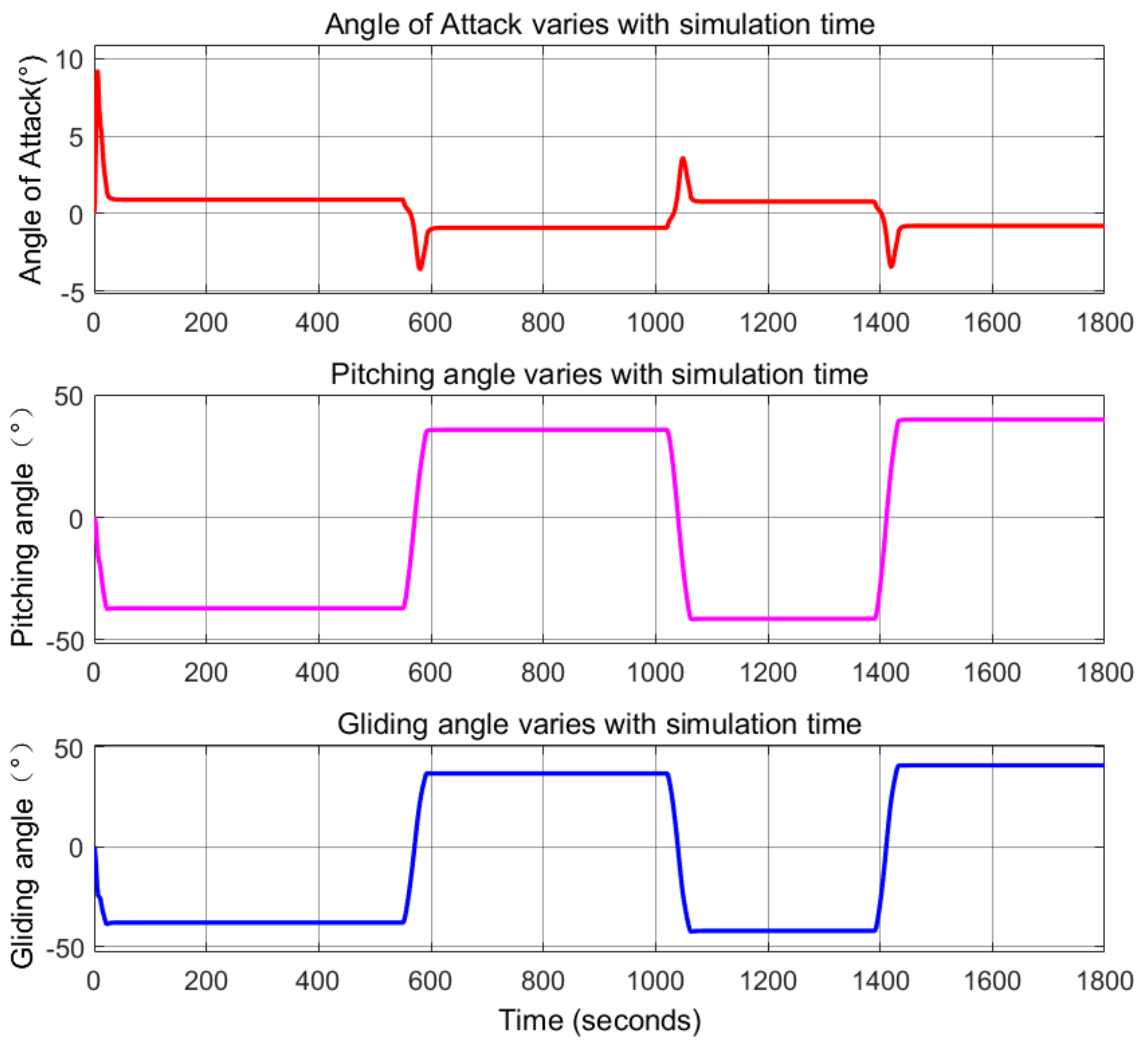
The piston was operated by the transmission motor; it propagated inward or outward from the initial equilibrium state, and the buoyancy engine began to absorb or drain water. The glider was subject to the net buoyancy and hydrodynamic forces, and it dove or floated in the water. Based on the simulation results, the trends of the pitch angle, AOA, and gliding angle of the glider were obtained. The UG adjusted the underwater navigation attitude via the buoyancy engine and movable mass, and the gliding attitude angle changed with the variations in the buoyancy engine and movable mass.

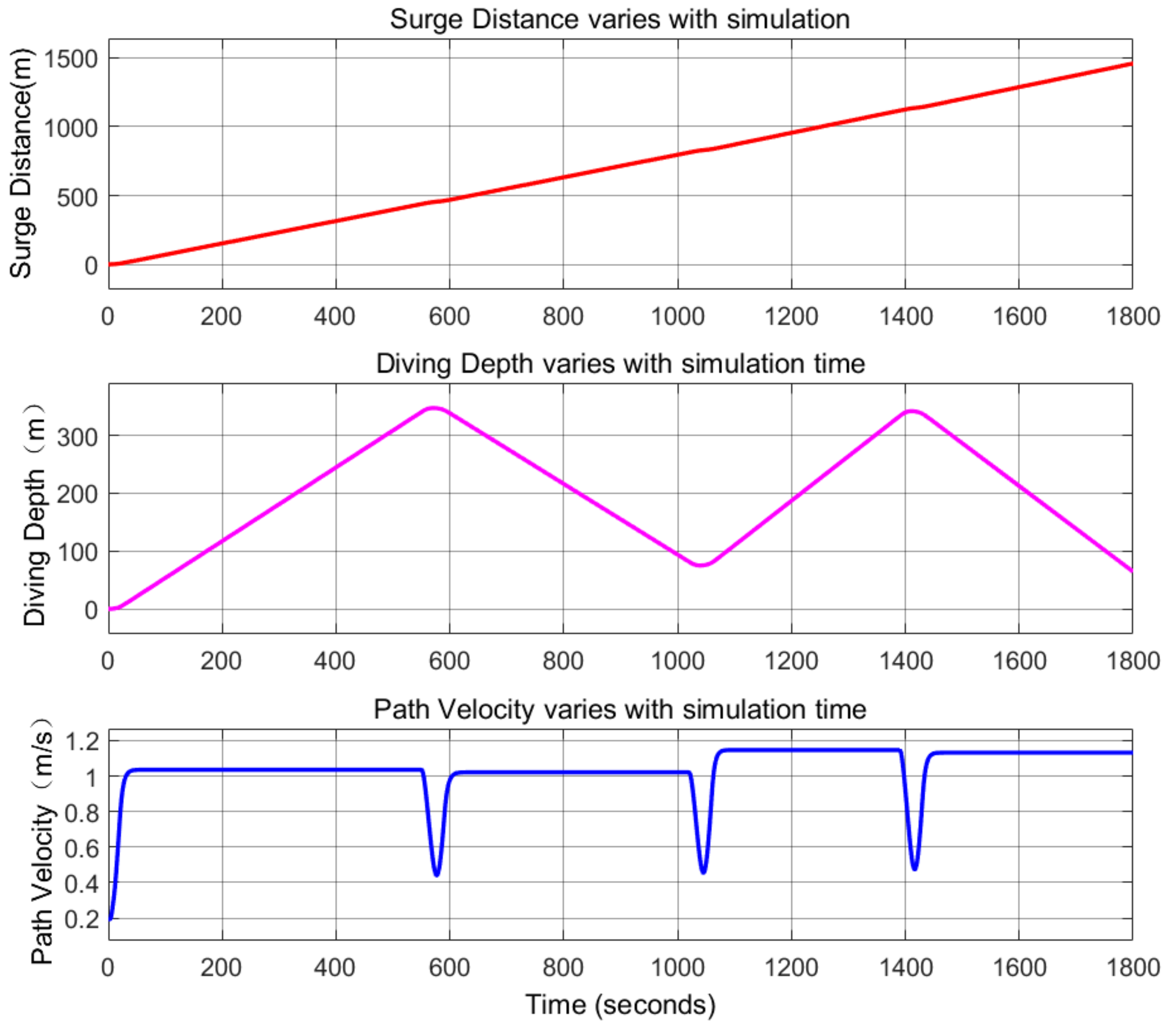
Figure 7 presents the change in angle with the simulation time when the UG glided upward or downward. Figure 8 presents the surge, diving, and path velocity varying with the simulation time when the UG glided upward or downward. The horizontal coordinate of the figure indicates the simulation time, and two motion cycles were observed, i.e., diving followed by surfacing.

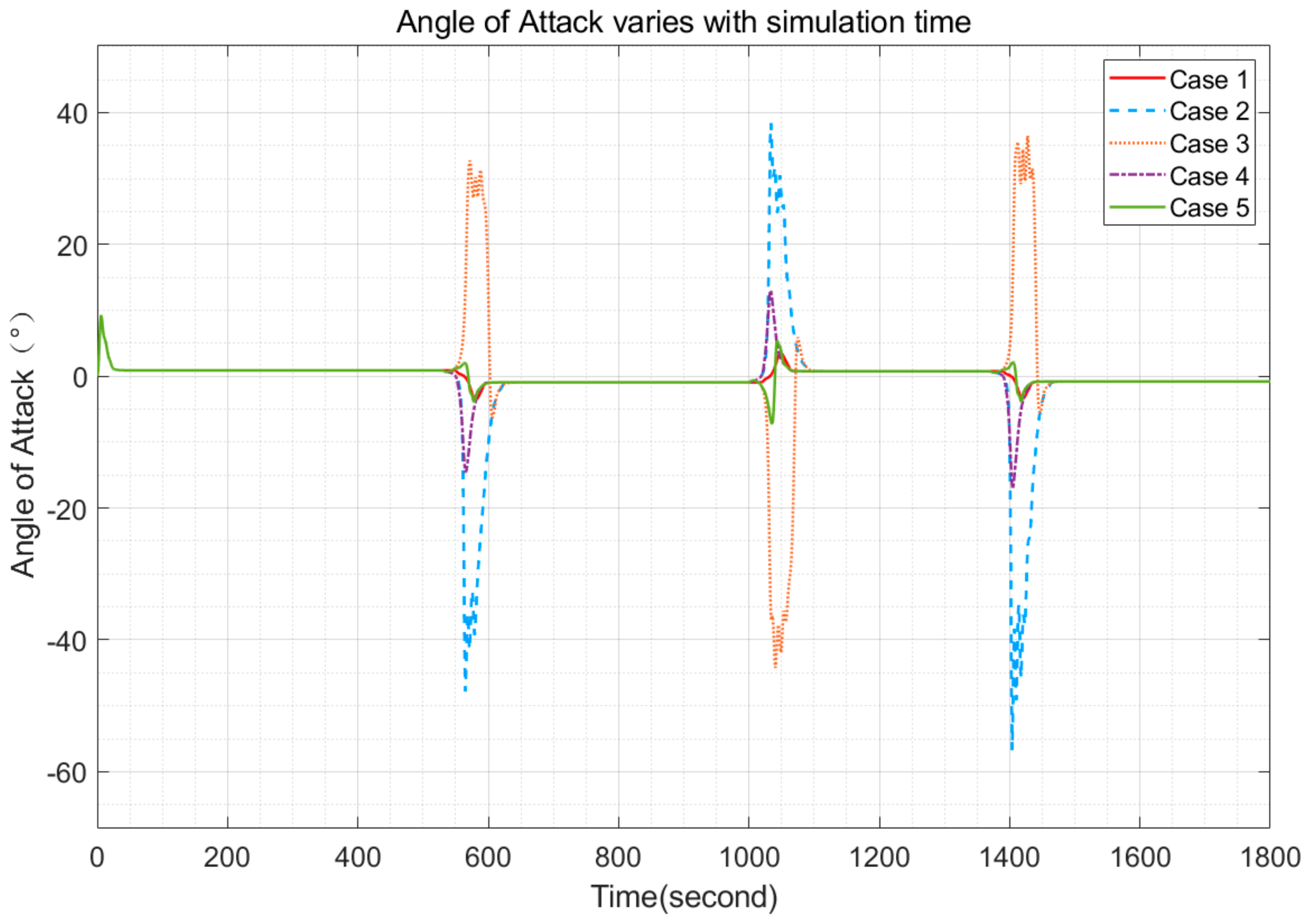
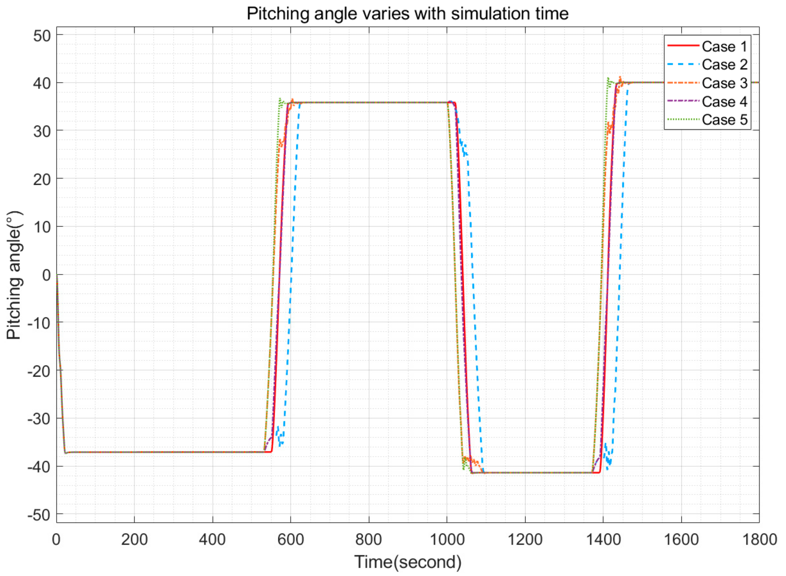
Based on the above model, the effect of the interrelationship between the movable mass block and the displacement variation of the piston assembly on the angle of attack and the pitch angle was further investigated. The following five displacement change relationships were simulated here, namely case 1, where the movable mass block moves and stops simultaneously with the piston assembly; case 2, where the piston assembly moves first and the movable mass block starts moving after the piston assembly stops; case 3, where the piston and movable mass block move in the opposite relationship to case 2; case 4, where the piston assembly moves first and the movable mass block starts moving before the piston assembly stops; and case 5, where the piston moves in relation to the movable mass block in the opposite way to case 4. From the changes of angle of attack and pitch angle during attitude transformation in Figure 9 and Figure 10, it can be seen that the fluctuation of angle occurs during attitude adjustment, while in case 1, the glide angle parameters change smoothly, and it can be considered that such state has the best attitude control effect. Figure 9 and Figure 10 show the variation of angles.

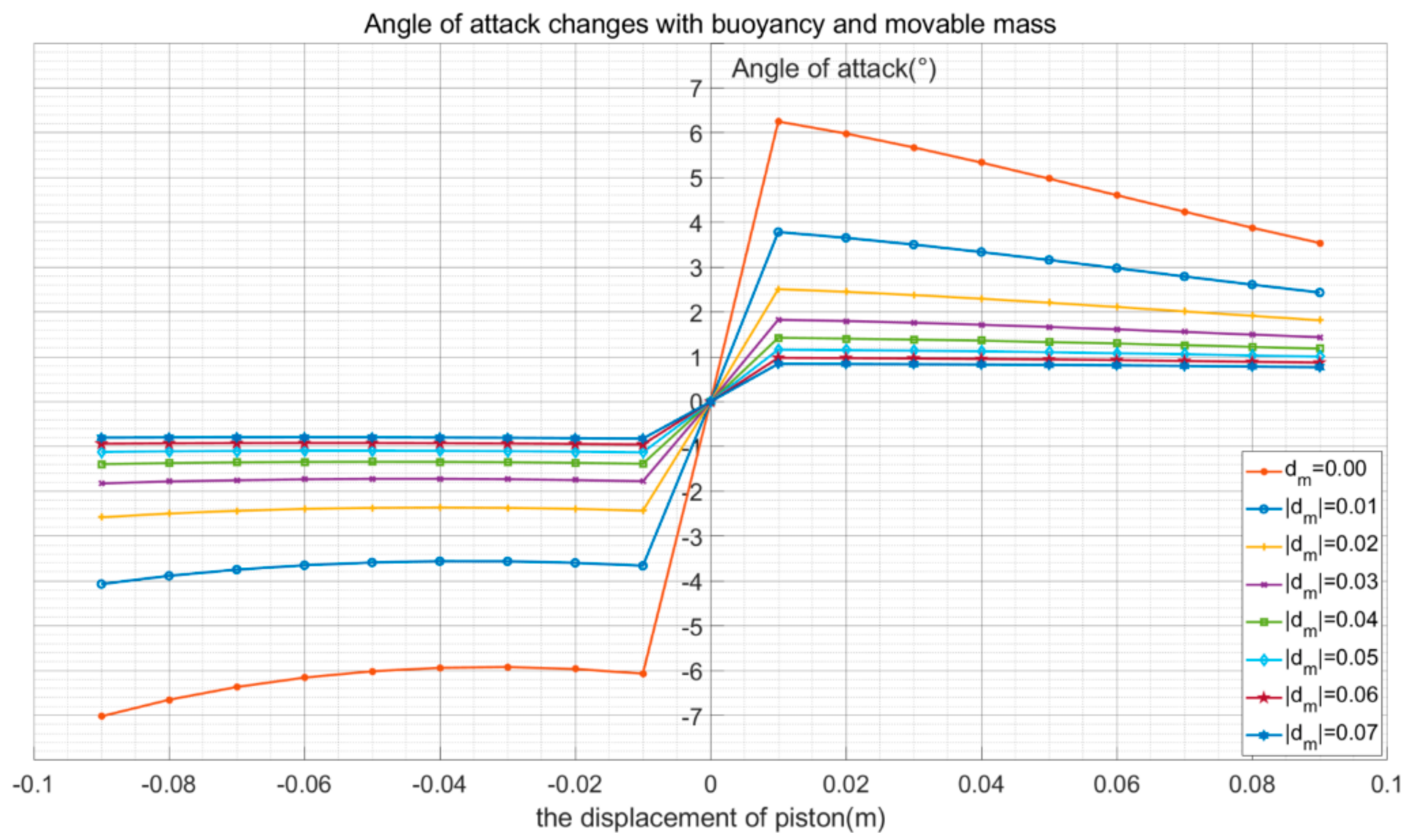
The relationship among the attitude angle, buoyancy engine, and movable mass was obtained from the motion simulation (see Figure 11). The AOA changed with the buoyancy and movable mass when the UG glided downward and upward. The horizontal coordinate in the figure indicates the displacement of the piston, i.e., the positive and negative regions represent the piston drawing inward and draining outward, respectively. The legend of the figure shows the displacement of the movable mass. The left-half plane indicates that the glider glides upward and the movable mass moves backward, whereas the right-half plane indicates that the glider dives downward and the movable mass moves forward.

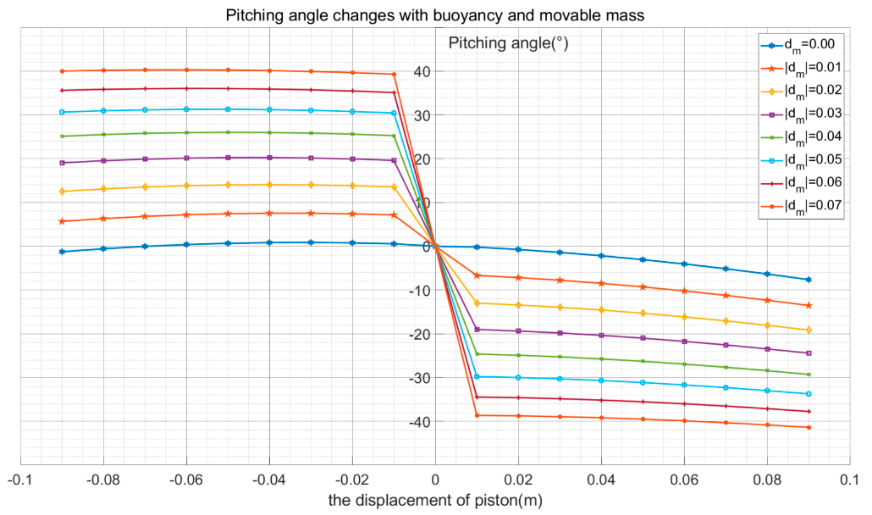
Figure 12 shows that the pitching angle changes with the buoyancy and the movable mass when the UG glides downward and upward. The horizontal coordinate of the figure indicates the displacement of the piston, i.e., the positive and negative regions represent the piston drawing inward and draining outward, respectively. The legend of the figure shows the displacement of the movable slider. The left-half plane indicates that the glider glides upward and the movable mass moves backward, whereas the right-half plane indicates that the glider dives downward and the movable mass moves forward.

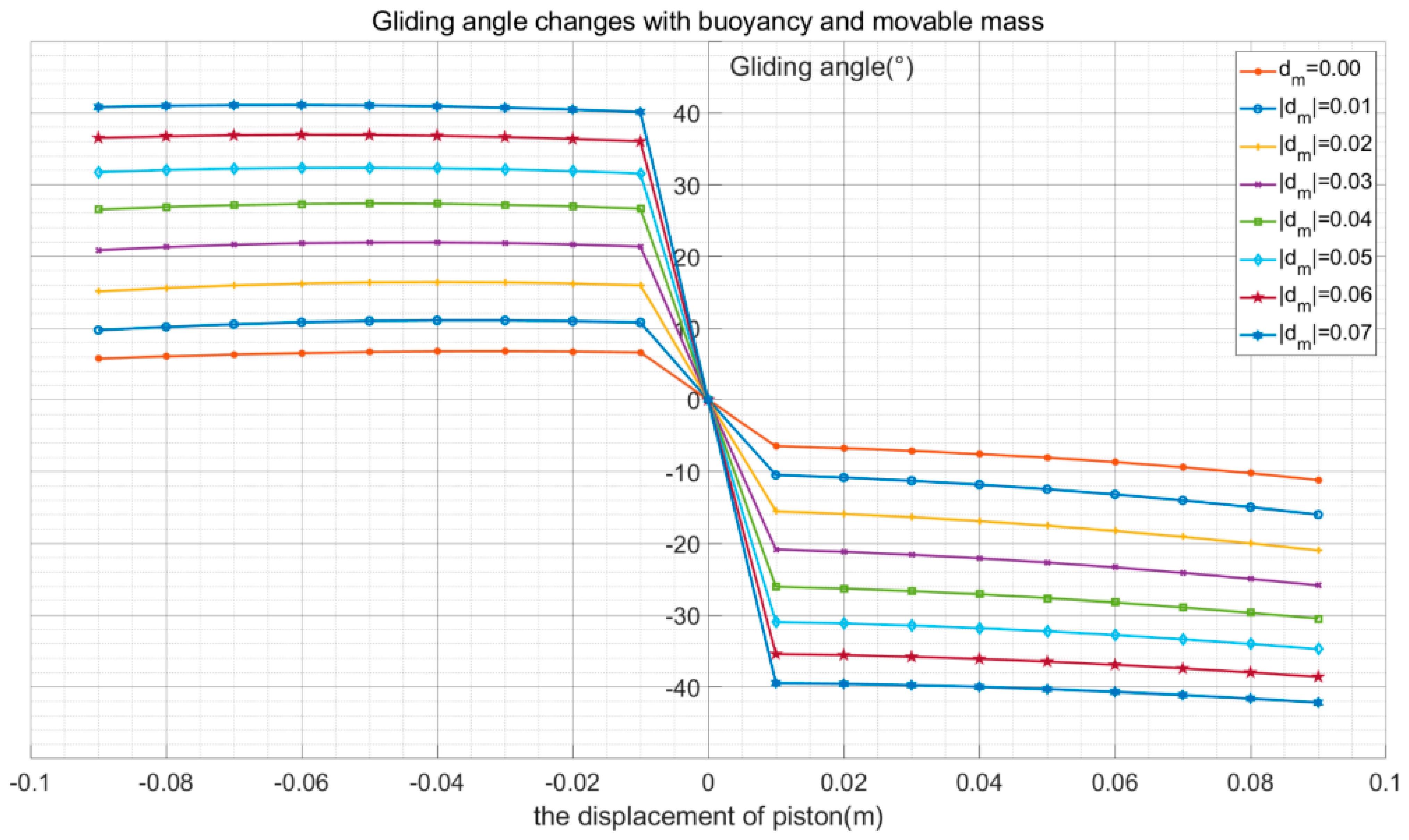
Figure 13 presents the change in the gliding angle with the buoyancy and movable mass when the UG glides upward or downward. The horizontal coordinate of the figure indicates the displacement of the piston, i.e., the positive and negative regions represent the piston drawing inward and draining outward, respectively. The legend of the figure shows the displacement of the movable slider. The left-half plane indicates that the glider glides upward and the movable mass moves backward, whereas the right-half plane indicates that the glider dives downward and the movable mass moves forward.

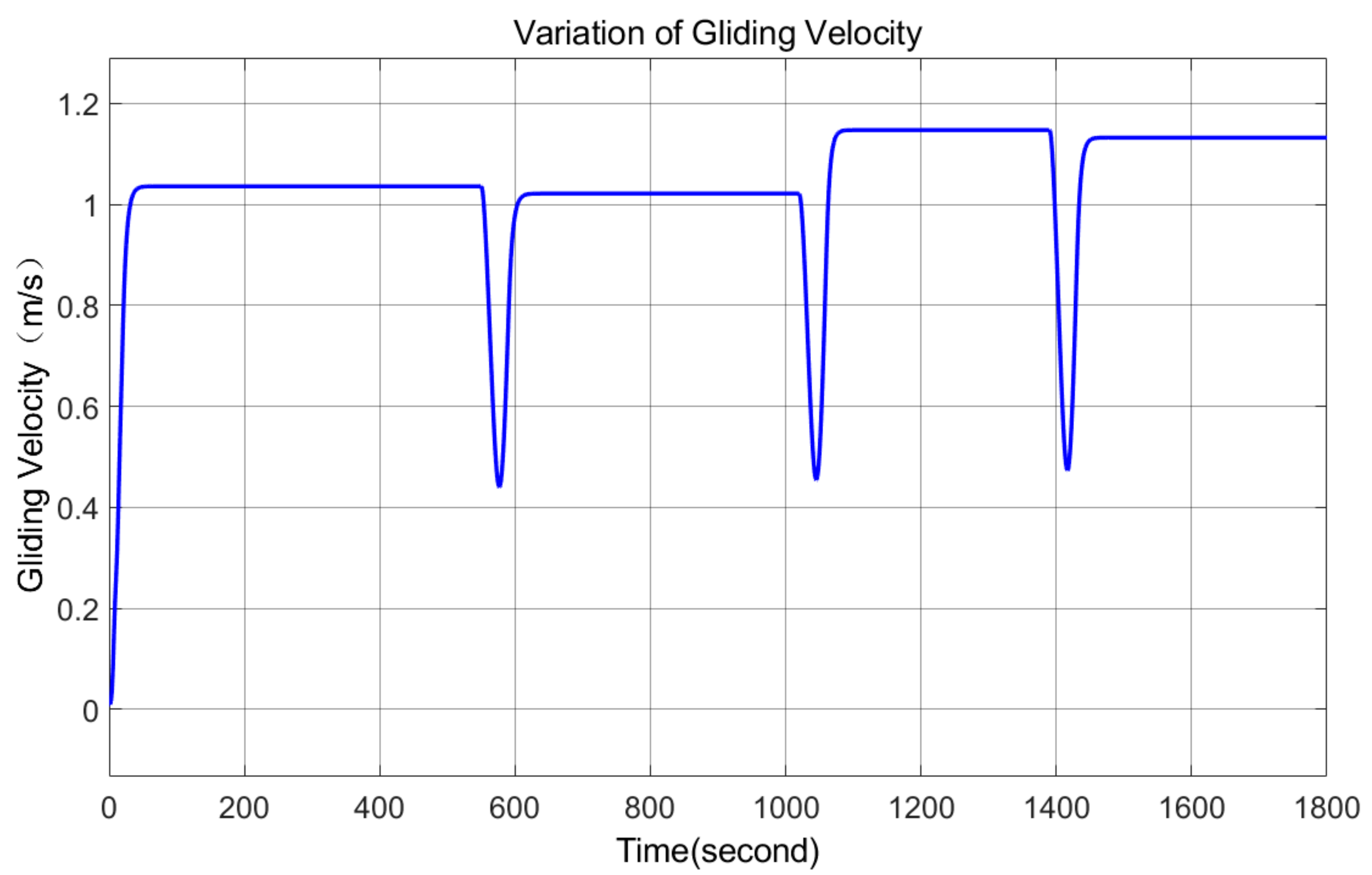
The path speed of the glider indicated the maximum value when the gliding angle was 35°. Based on the trend of the gliding angle shown in Figure 13, the displacement of the movable mass and piston corresponding to the instant the glider reached the maximum gliding speed can be derived. In this study, the glider motion was simulated in two cycles, i.e., diving followed by surfacing. Figure 14 shows the variation in the gliding speed during the simulation.

5. Experiment

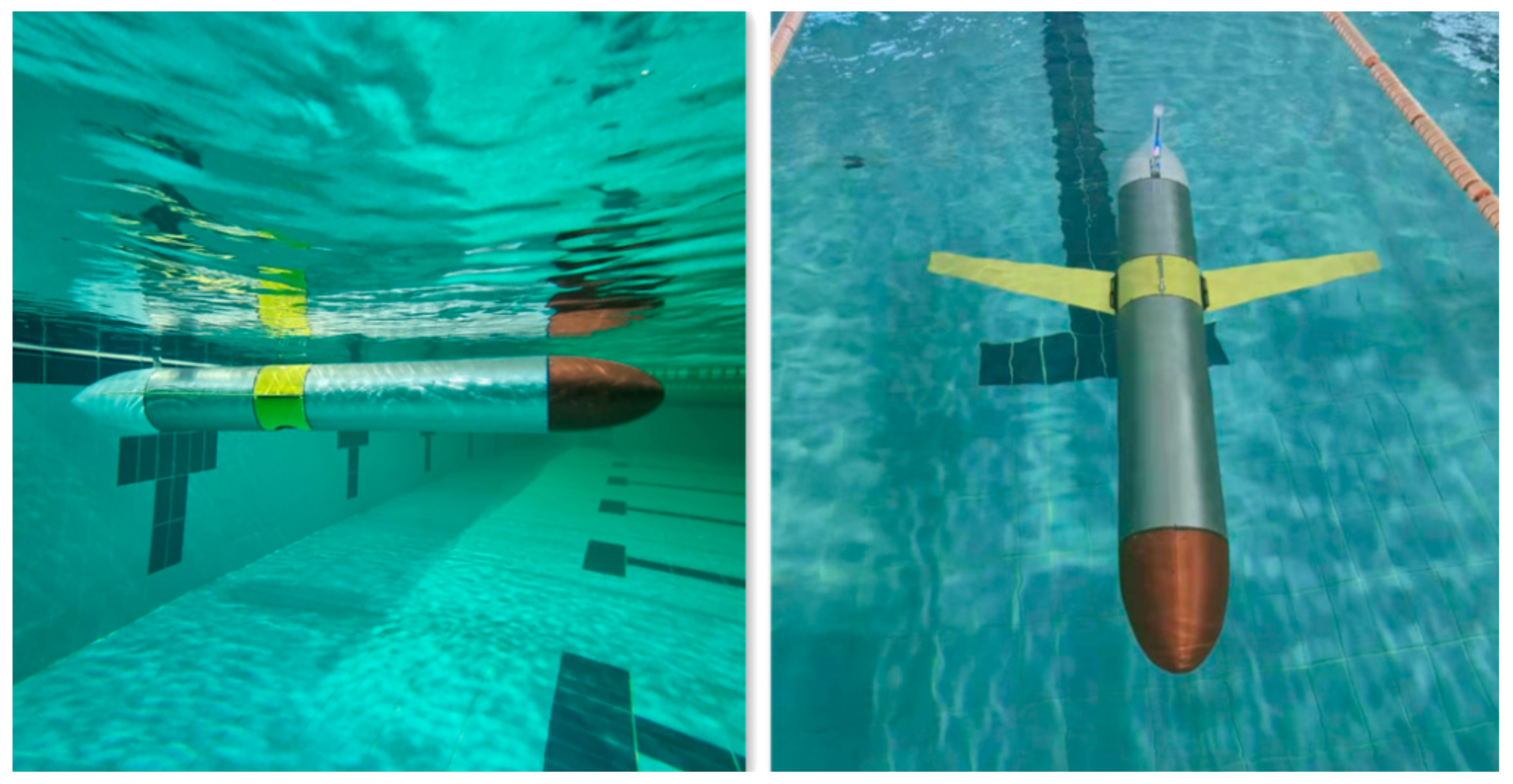
To verify the feasibility of the glider structure design, a simple experiment was conducted to investigate the variation in the glider pitch angle with the movable mass block owing to the limitations of the experimental conditions. Due to the communication needs, the antenna part must be exposed above the water surface, which means that the glider cannot be completely submerged in water, which is why the ballast water mass obtained from the experiment is not the same as the ballast water mass in the aforementioned Table 1. This experiment only tests the change of the pitch angle of the glider after the movable mass block is moved when the glider floats on the water surface. The experiment was conducted in the university swimming pool, and the deepest depth of the pool was 3 m, which does not satisfy the gliding experiment requirements. Figure 15 shows photographs of the experimental site.

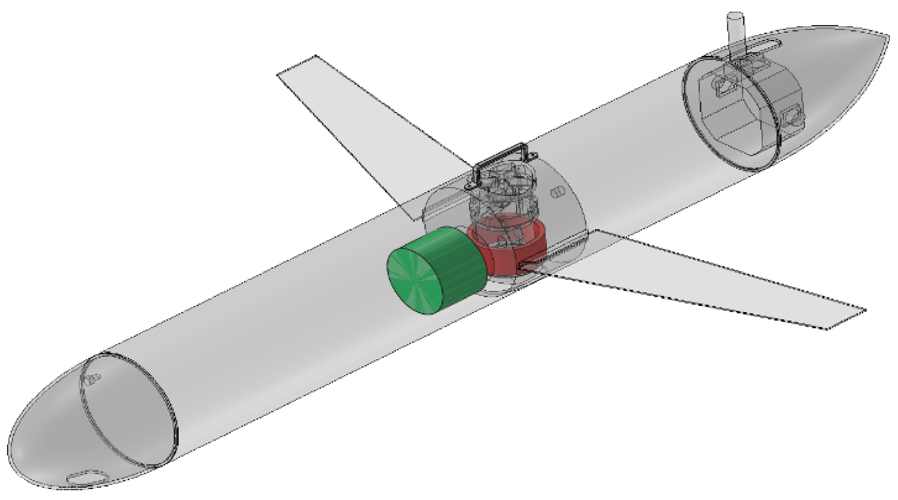
The middle section (yellow sector) shown in the photographs above contained communication cables. The total length of the cables was 2800 mm, their diameter was 10 mm, and the buoyancy of the cables was modeled as an equivalent circle (red model), as shown in Figure 15. The glider was not completely submerged in water, which implies that the antenna housing appeared partially above the water. The buoyancy of the glider is illustrated in Figure 16. The green part represents the ballast water in the buoyancy cylinder whose mass was 1.98 kg.

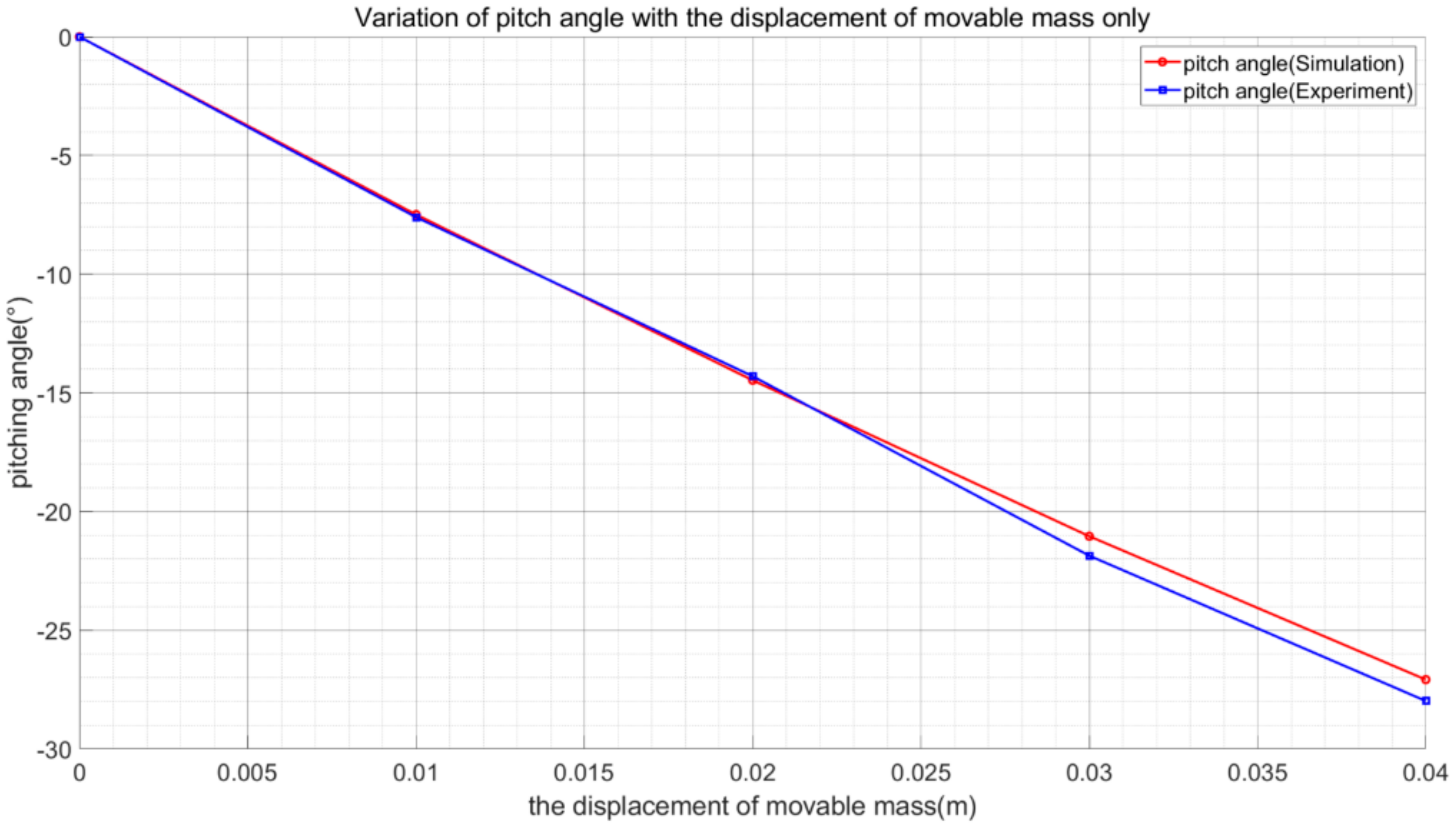
First, the glider was suspended horizontally in water by the buoyancy adjustment mechanism and the movable mass block; at the end of the experiment, the distance from the surface of the piston to the end face of the buoyancy cylinder in the buoyancy engine was measured so that the mass of ballast water in the buoyancy engine for this experiment could be calculated; subsequently, the buoyancy mechanism was maintained, and the experimental values of the pitch angle under different attitudes were obtained by adjusting the different positions of the movable mass block, in which the movable mass block moved 10 mm each time. During the motion of the movable mass, the pitch angle was recorded at each moment using the built-in sensor on board, and after the experiment, the data were exported and fitted to produce a relationship between the pitch angle and the displacement of the movable mass. Next, the experimental results were compared with the simulation results. Owing to the limitations of the experiment, only the comparative results of the forward motion of the movable mass block are shown herein. The comparison results showed that the simulation and experimental results agreed well, with a maximum error of less than 1°. By comparing the model with the physical glider, the analysis concluded that this error should be caused by the distribution of the cables inside the fuselage. We can only measure the mass and the approximate location distribution of the cables, but we cannot easily reproduce the distribution of the cables inside the fuselage with the modeling software. More detailed results will be described in a future paper. The comparative results of the experimental and simulation results are shown below Figure 17.

6. Conclusions

In this study, a UG that can dive to a depth of 400 m at a cruising speed of 2 knots was investigated. The motion of the UG with respect to the position variation of the internal movable mass and piston cylinder pump was analyzed. The hull profile of the glider was designed using the MYRING equations. The hydrodynamic parameters of the glider were obtained based on computer simulation using SolidWorks. By analyzing the mass distribution of each component in the glider, two reference coordinate systems were established for the underwater glider, different from the motion models of other references, the displacements of the movable mass block ($d_{\overline{m}1}$), and the piston assembly ($d_{p1}$) in the x-axis of body coordinate as inputs for the simulation, and the equations of motion of the glider in the vertical plane were derived and simulated using MATLAB and Simulink. An underwater glider was constructed to validate the simulation analysis, and experiments were conducted.

The simulation results indicated that the AOA changed rapidly with the position change of the movable mass, i.e., the larger the displacement of the movable mass, the smaller the AOA, and the smoother the change in the AOA. In addition, as the displacement of the movable mass increased, the buoyant effect on the AOA diminished gradually. The movable mass significantly affected the pitching angle, where a larger mass and displacement resulted in a more significant change in the pitching angle. The results showed that the pitch angle varied approximately linearly with the displacement of the piston in the glider dive stage and that the pitch angle changed by approximately 1° for every 10 mm movement of the piston. However, the displacement of the piston imposed a less significant effect on the pitch angle when the glider was surfacing. In the glider diving or surfacing stage, the pitch angle changed linearly with the displacement of the movable mass, and the pitch angle changed by approximately 7° for every 10 mm movement of the movable mass; however, as the displacement of the movable mass block increased, the change in pitch angle decreased slowly. The effects of the displacements of the piston and movable mass block on the glide angle were consistent with the pitch angle results. From the contents of Figure 10 and Figure 11, it can be obtained that under five different conditions, the glider showed different magnitude fluctuations in the angle of attack and pitch angle during the attitude switching; keeping the consistency of the piston and movable mass block can make the glider behave more stably in the attitude transformation; and the simulation results can be used as reference data for the attitude control of the UG. For the pitching experiments involving the adjustments of different positions of the movable mass block, the maximum pitching angle error was less than 1°, which indicates the excellent modeling of the glider.