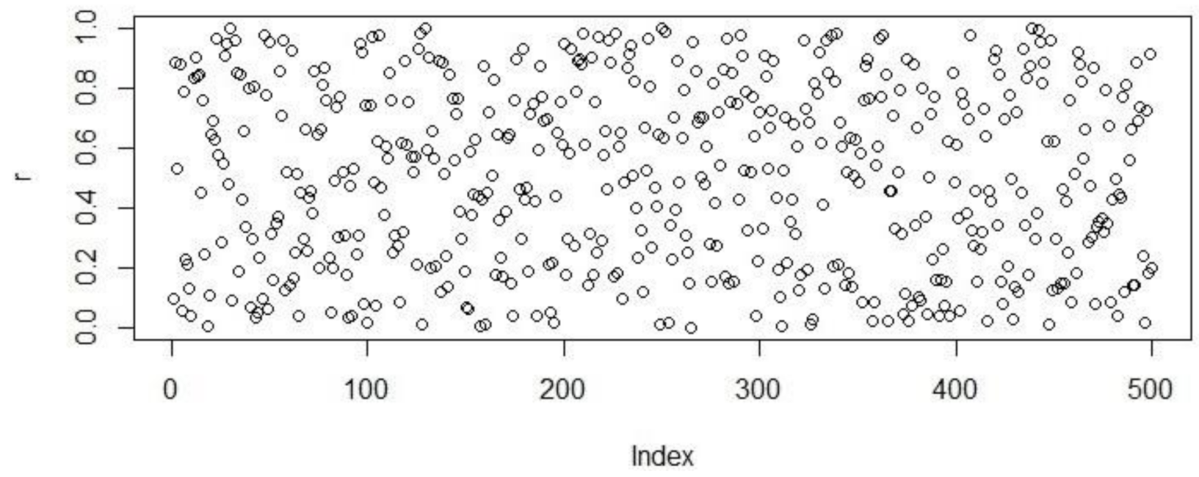
Figure 1.
Population initialization using uniform distribution.
Figure 1.
Population initialization using uniform distribution.
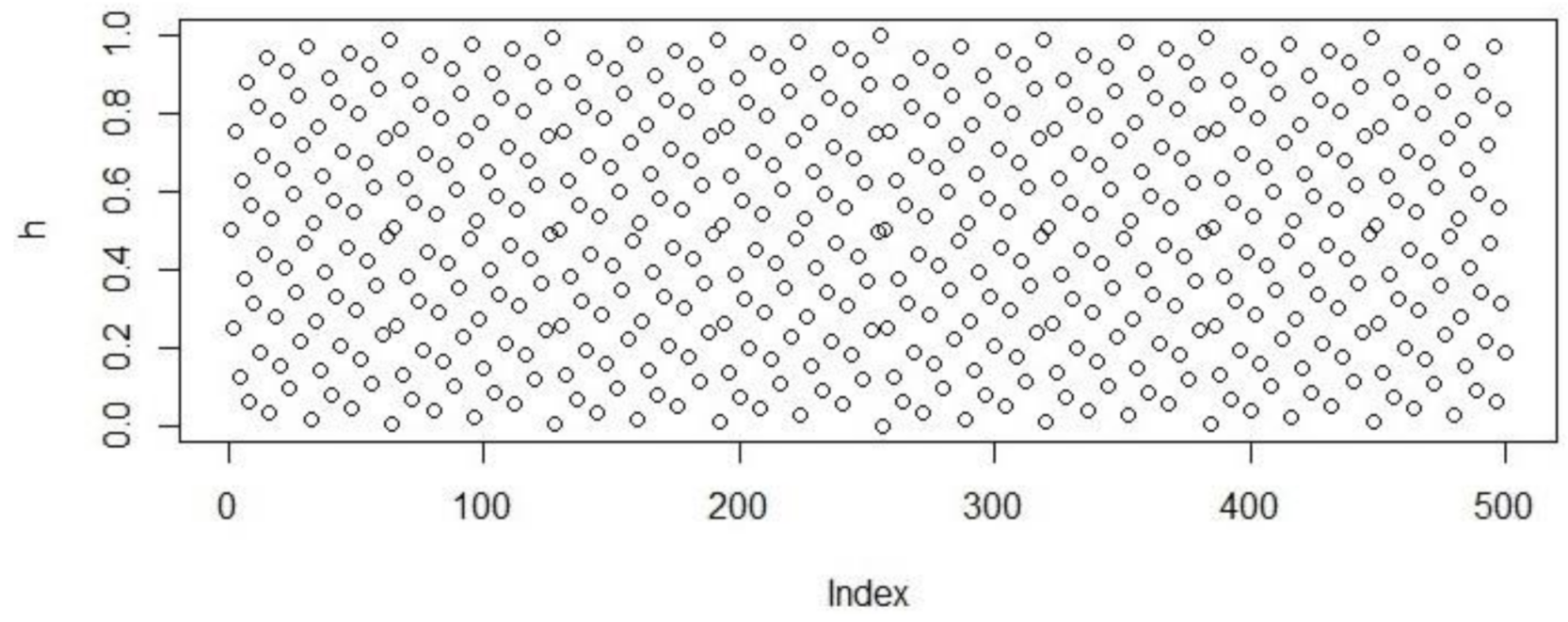
Figure 2.
Population initialization using Sobol distribution.
Figure 2.
Population initialization using Sobol distribution.
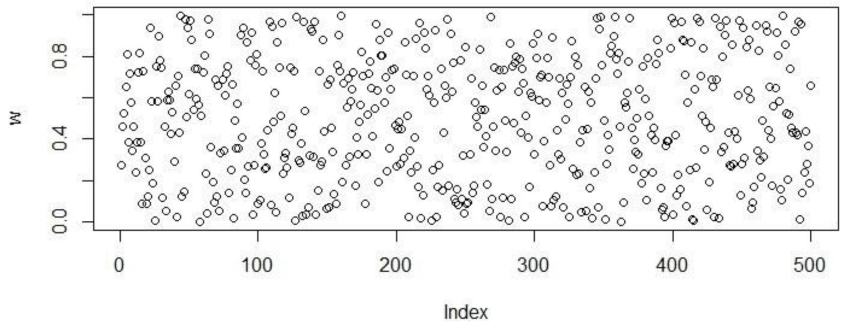
Figure 3.
Population initialization using Halton distribution.
Figure 3.
Population initialization using Halton distribution.
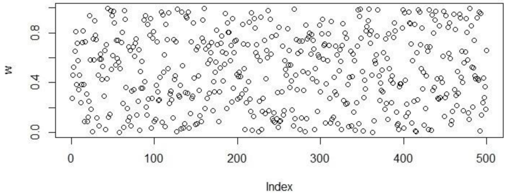
Figure 4.
Population initialization using WELL distribution.
Figure 4.
Population initialization using WELL distribution.
Figure 5.
Population initialization using Knuth distribution.
Figure 5.
Population initialization using Knuth distribution.
Figure 6.
Sample data generated using Torus distribution.
Figure 6.
Sample data generated using Torus distribution.
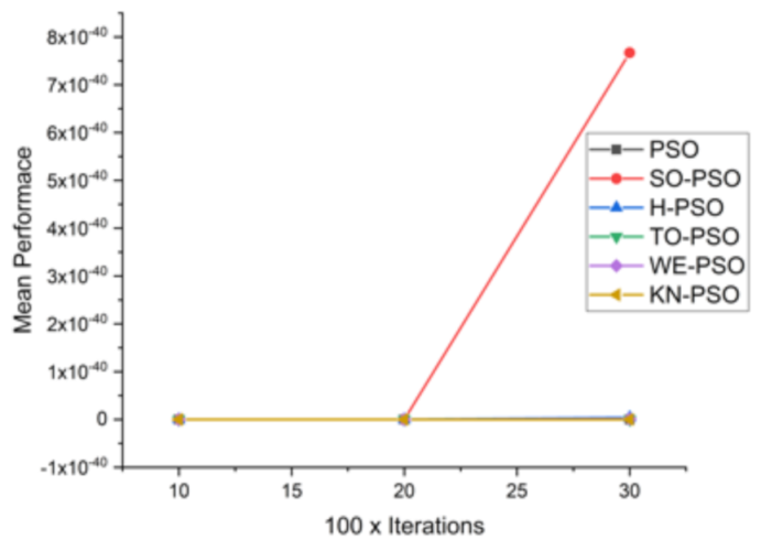
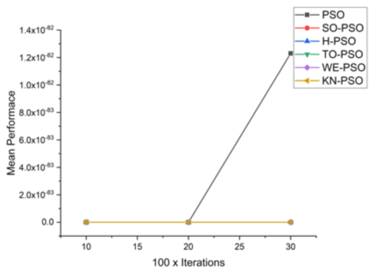
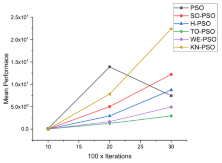
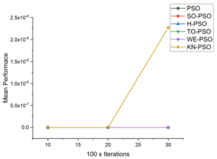
Figure 7.
Convergence curve on F1.
Figure 7.
Convergence curve on F1.
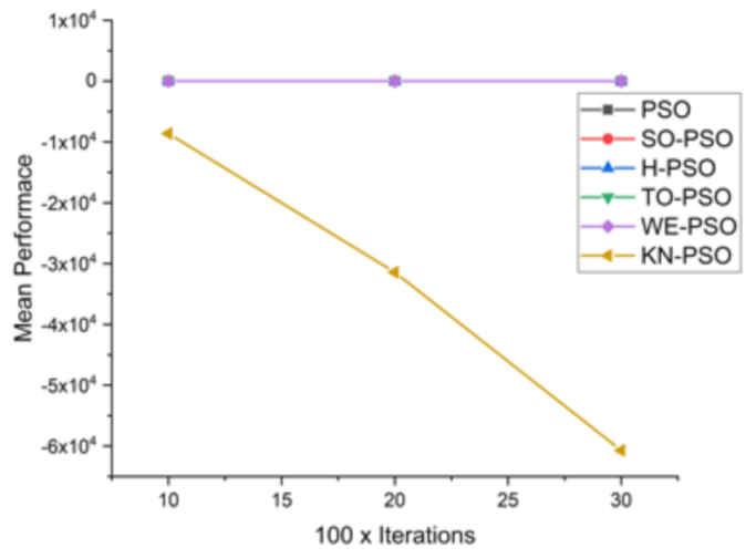
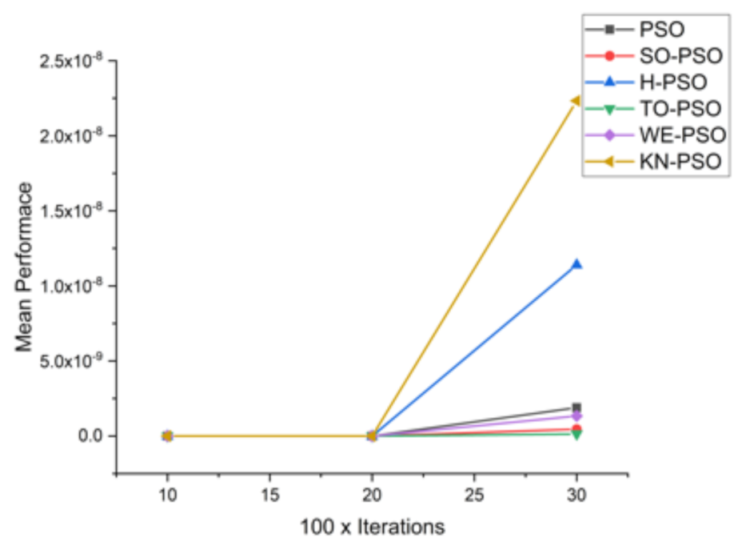
Figure 8.
Convergence curve on F2.
Figure 8.
Convergence curve on F2.
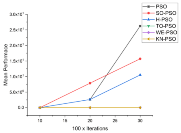
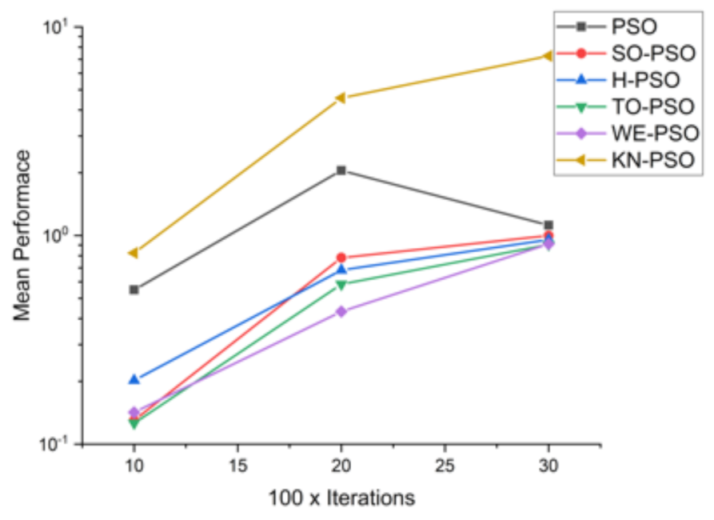
Figure 9.
Convergence curve on F3.
Figure 9.
Convergence curve on F3.
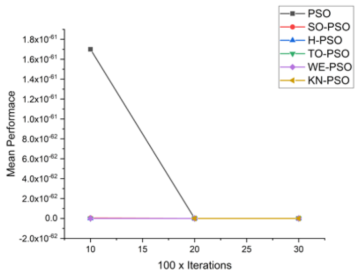
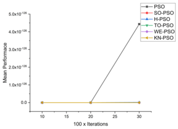
Figure 10.
Convergence curve on F4.
Figure 10.
Convergence curve on F4.
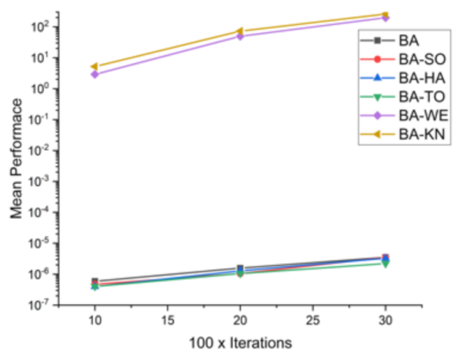
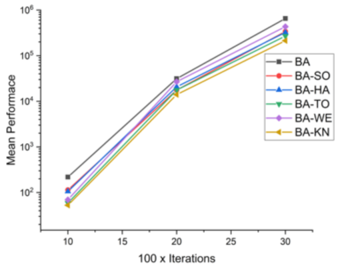
Figure 11.
Convergence curve on F5.
Figure 11.
Convergence curve on F5.
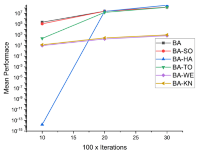
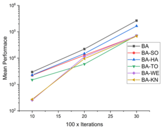
Figure 12.
Convergence curve on F6.
Figure 12.
Convergence curve on F6.
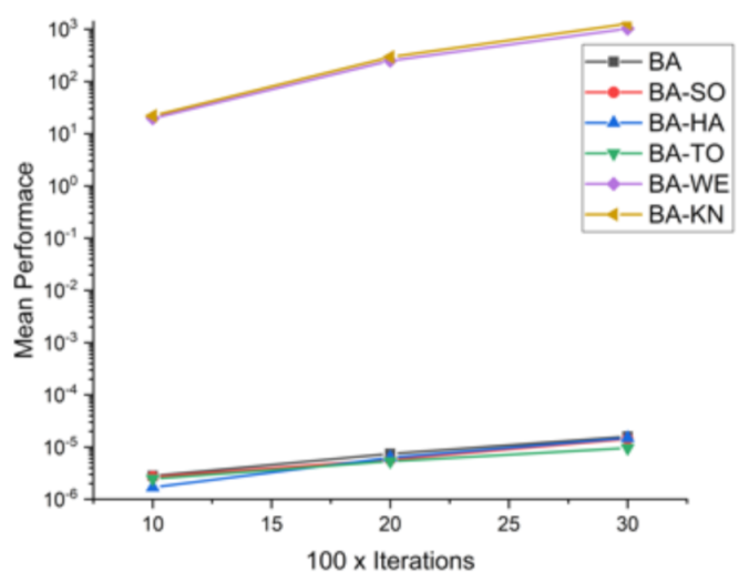
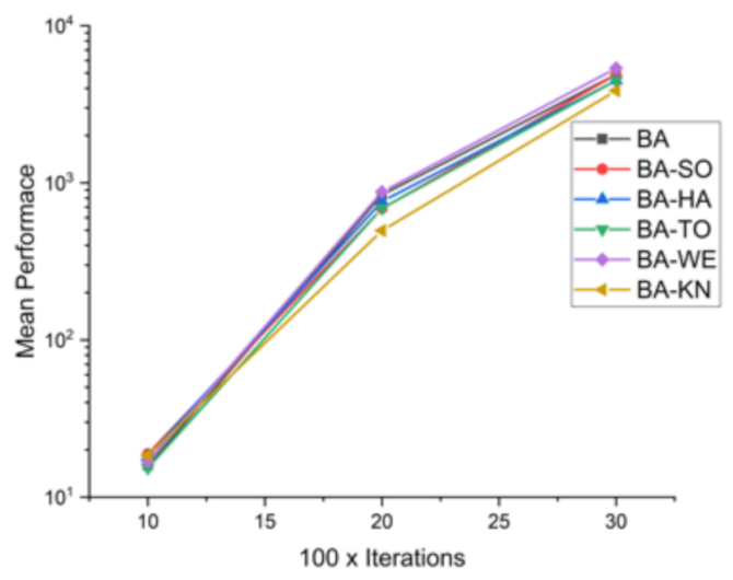
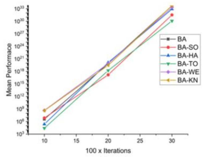
Figure 13.
Convergence curve on F7.
Figure 13.
Convergence curve on F7.
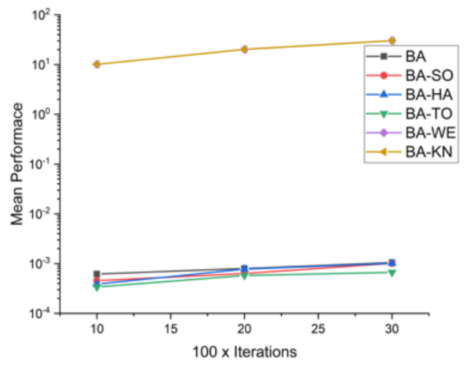
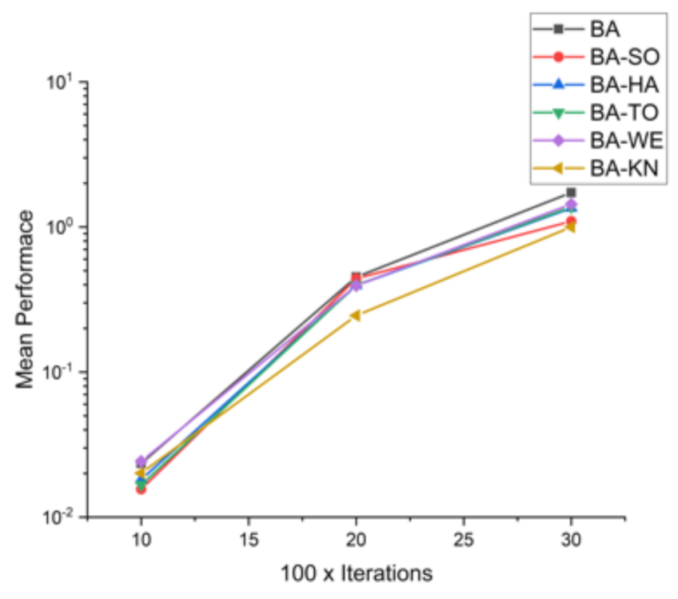
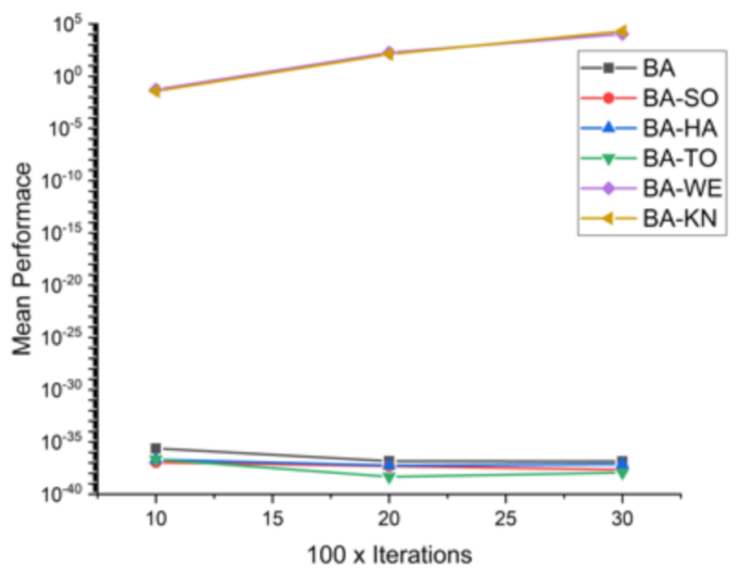
Figure 14.
Convergence curve on F8.
Figure 14.
Convergence curve on F8.
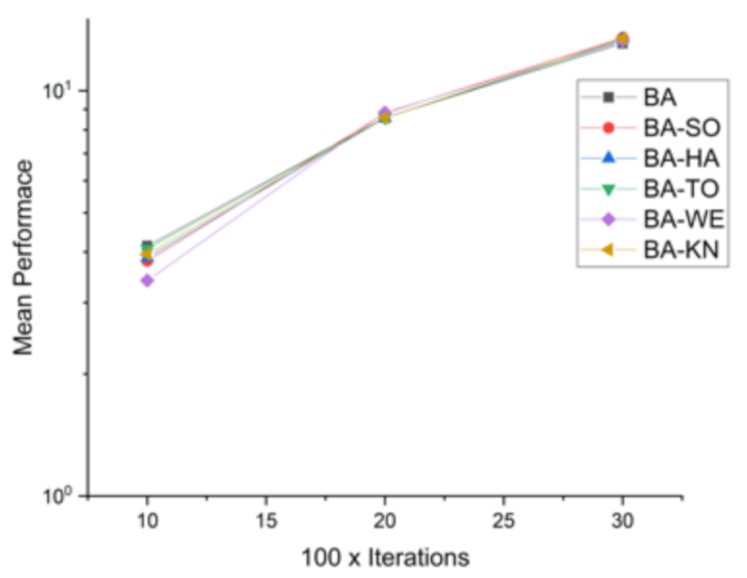
Figure 15.
Convergence curve on F9.
Figure 15.
Convergence curve on F9.
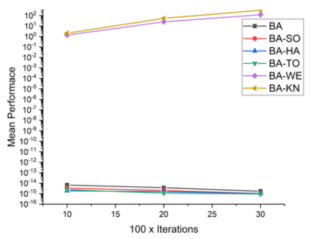
Figure 16.
Convergence curve on F10.
Figure 16.
Convergence curve on F10.
Figure 17.
Convergence curve on F11.
Figure 17.
Convergence curve on F11.
Figure 18.
Convergence curve on F12.
Figure 18.
Convergence curve on F12.
Figure 19.
Convergence curve on F13.
Figure 19.
Convergence curve on F13.
Figure 20.
Convergence curve on F14.
Figure 20.
Convergence curve on F14.
Figure 21.
Convergence curve on F15.
Figure 21.
Convergence curve on F15.
Figure 22.
Convergence curve on F16.
Figure 22.
Convergence curve on F16.
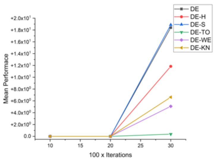
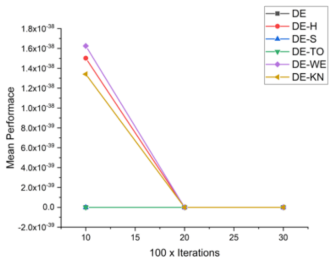
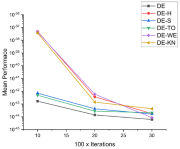
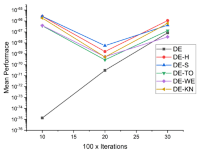
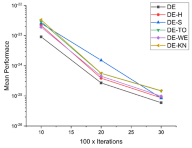
Figure 23.
Convergence curve on F1.
Figure 23.
Convergence curve on F1.
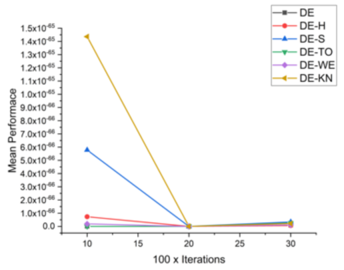
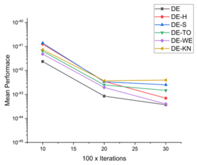
Figure 24.
Convergence curve on F2.
Figure 24.
Convergence curve on F2.
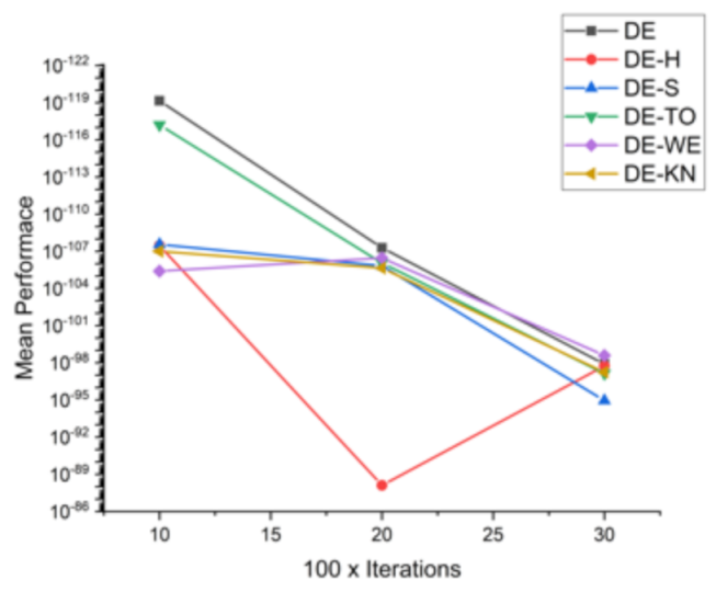
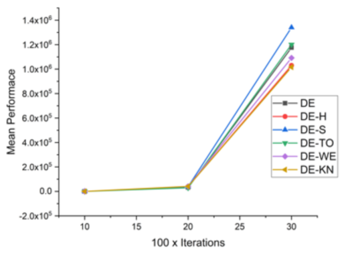
Figure 25.
Convergence curve on F3.
Figure 25.
Convergence curve on F3.
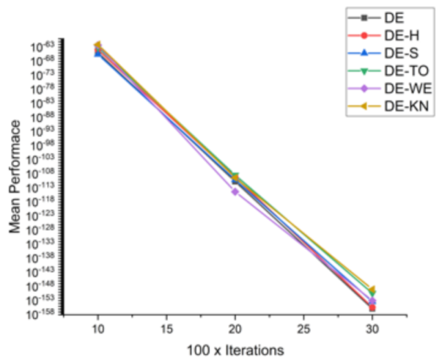
Figure 26.
Convergence curve on F4.
Figure 26.
Convergence curve on F4.
Figure 27.
Convergence curve on F5.
Figure 27.
Convergence curve on F5.
Figure 28.
Convergence curve on F6.
Figure 28.
Convergence curve on F6.
Figure 29.
Convergence curve on F7.
Figure 29.
Convergence curve on F7.
Figure 30.
Convergence curve on F8.
Figure 30.
Convergence curve on F8.
Figure 31.
Convergence curve on F9.
Figure 31.
Convergence curve on F9.
Figure 32.
Convergence curve on F10.
Figure 32.
Convergence curve on F10.
Figure 33.
Convergence curve on F11.
Figure 33.
Convergence curve on F11.
Figure 34.
Convergence curve on F12.
Figure 34.
Convergence curve on F12.
Figure 35.
Convergence curve on F13.
Figure 35.
Convergence curve on F13.
Figure 36.
Convergence curve on F14.
Figure 36.
Convergence curve on F14.
Figure 37.
Convergence curve on F15.
Figure 37.
Convergence curve on F15.
Figure 38.
Convergence curve on F16.
Figure 38.
Convergence curve on F16.
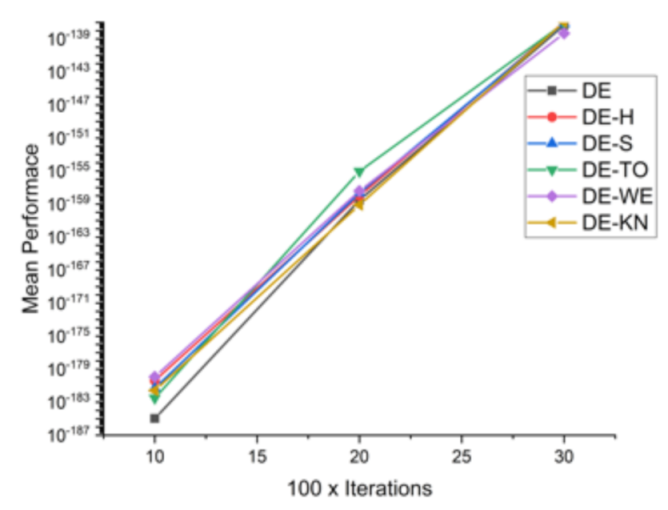
Figure 39.
Convergence curve on F1.
Figure 39.
Convergence curve on F1.
Figure 40.
Convergence curve on F2.
Figure 40.
Convergence curve on F2.
Figure 41.
Convergence curve on F3.
Figure 41.
Convergence curve on F3.
Figure 42.
Convergence curve on F4.
Figure 42.
Convergence curve on F4.
Figure 43.
Convergence curve on F5.
Figure 43.
Convergence curve on F5.
Figure 44.
Convergence curve on F6.
Figure 44.
Convergence curve on F6.
Figure 45.
Convergence curve on F7.
Figure 45.
Convergence curve on F7.
Figure 46.
Convergence curve on F8.
Figure 46.
Convergence curve on F8.
Figure 47.
Convergence curve on F9.
Figure 47.
Convergence curve on F9.
Figure 48.
Convergence curve on F10.
Figure 48.
Convergence curve on F10.
Figure 49.
Convergence curve on F11.
Figure 49.
Convergence curve on F11.
Figure 50.
Convergence curve on F12.
Figure 50.
Convergence curve on F12.
Figure 51.
Convergence curve on F13.
Figure 51.
Convergence curve on F13.
Figure 52.
Convergence curve on F14.
Figure 52.
Convergence curve on F14.
Figure 53.
Convergence curve on F15.
Figure 53.
Convergence curve on F15.
Figure 54.
Convergence curve on F16.
Figure 54.
Convergence curve on F16.
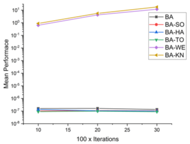
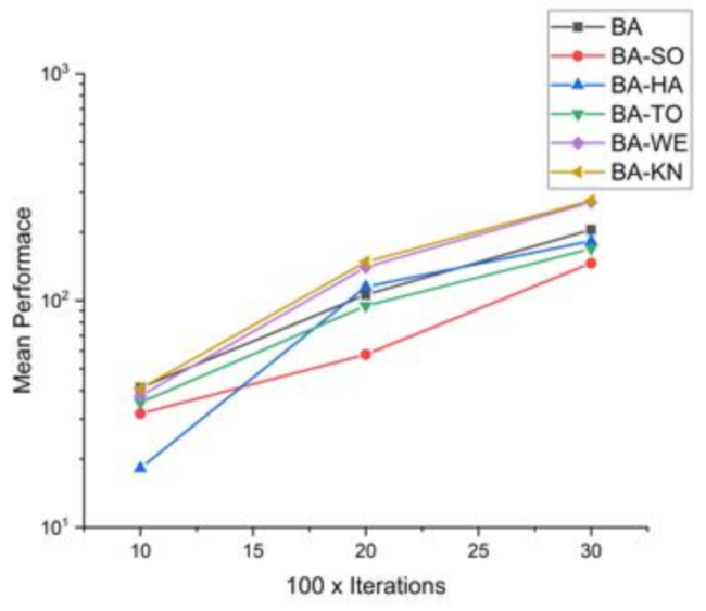
Figure 55.
Classification Testing Accuracy Results.
Figure 55.
Classification Testing Accuracy Results.
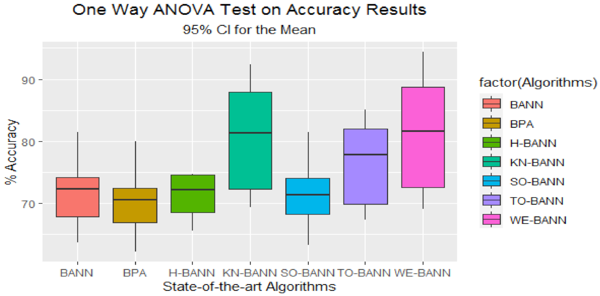
Figure 56.
Box plot visualization of the results achieved by the training of FFNN for all PSO-based initialization approaches and BPA for given datasets of the classification problem.
Figure 56.
Box plot visualization of the results achieved by the training of FFNN for all PSO-based initialization approaches and BPA for given datasets of the classification problem.
Figure 57.
Multi-comparison post-hoc Tukey test graph of all PSO-based.
Figure 57.
Multi-comparison post-hoc Tukey test graph of all PSO-based.
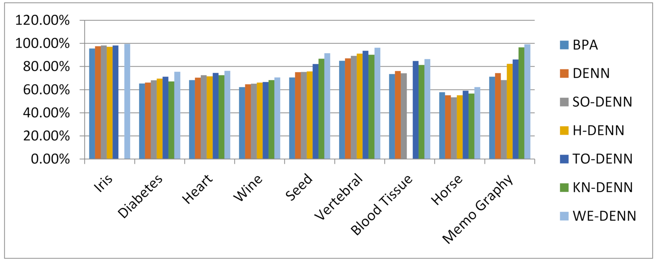
Figure 58.
Classification testing accuracy results.
Figure 58.
Classification testing accuracy results.
Figure 59.
Box plot visualization of the results achieved by the training of FFNN for all DE-based initialization approaches and BPA for given datasets of classification problem.
Figure 59.
Box plot visualization of the results achieved by the training of FFNN for all DE-based initialization approaches and BPA for given datasets of classification problem.
Figure 60.
Multi-comparison post-hoc Tukey test graph of all DE-based.
Figure 60.
Multi-comparison post-hoc Tukey test graph of all DE-based.
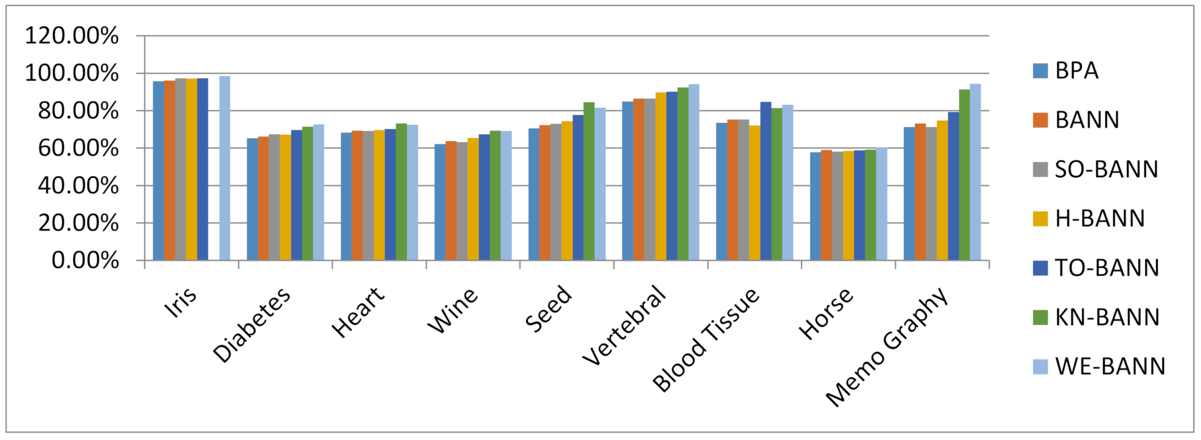
Figure 61.
Classification testing accuracy results.
Figure 61.
Classification testing accuracy results.
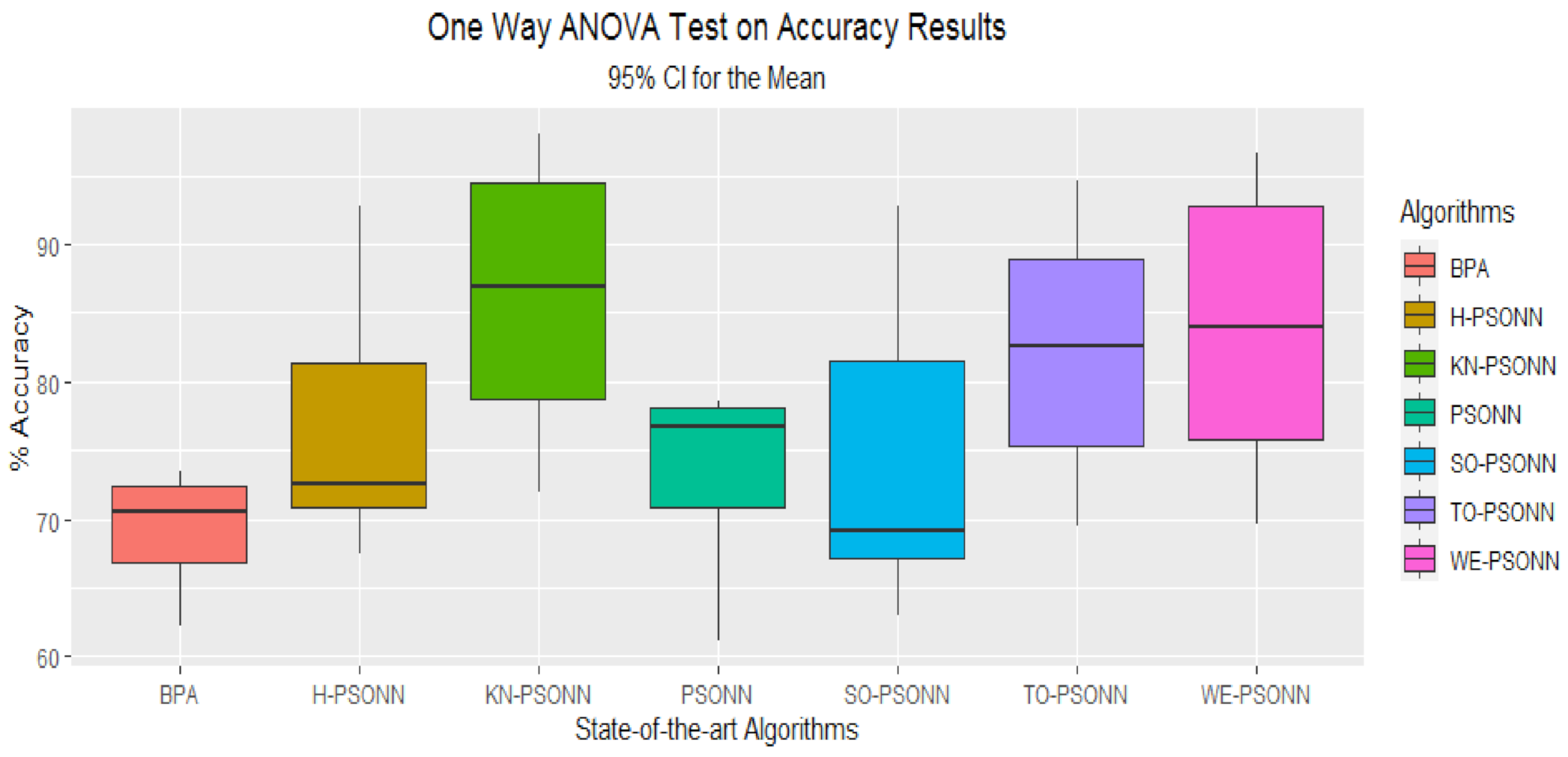
Figure 62.
Box plot visualization of the results achieved by the training of FFNN for all BA-based initialization approaches and BPA for given datasets of the classification problem.
Figure 62.
Box plot visualization of the results achieved by the training of FFNN for all BA-based initialization approaches and BPA for given datasets of the classification problem.
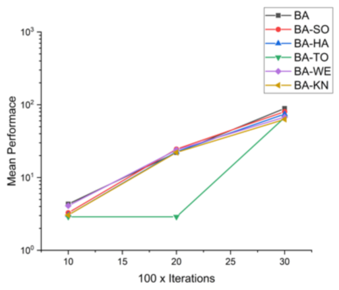
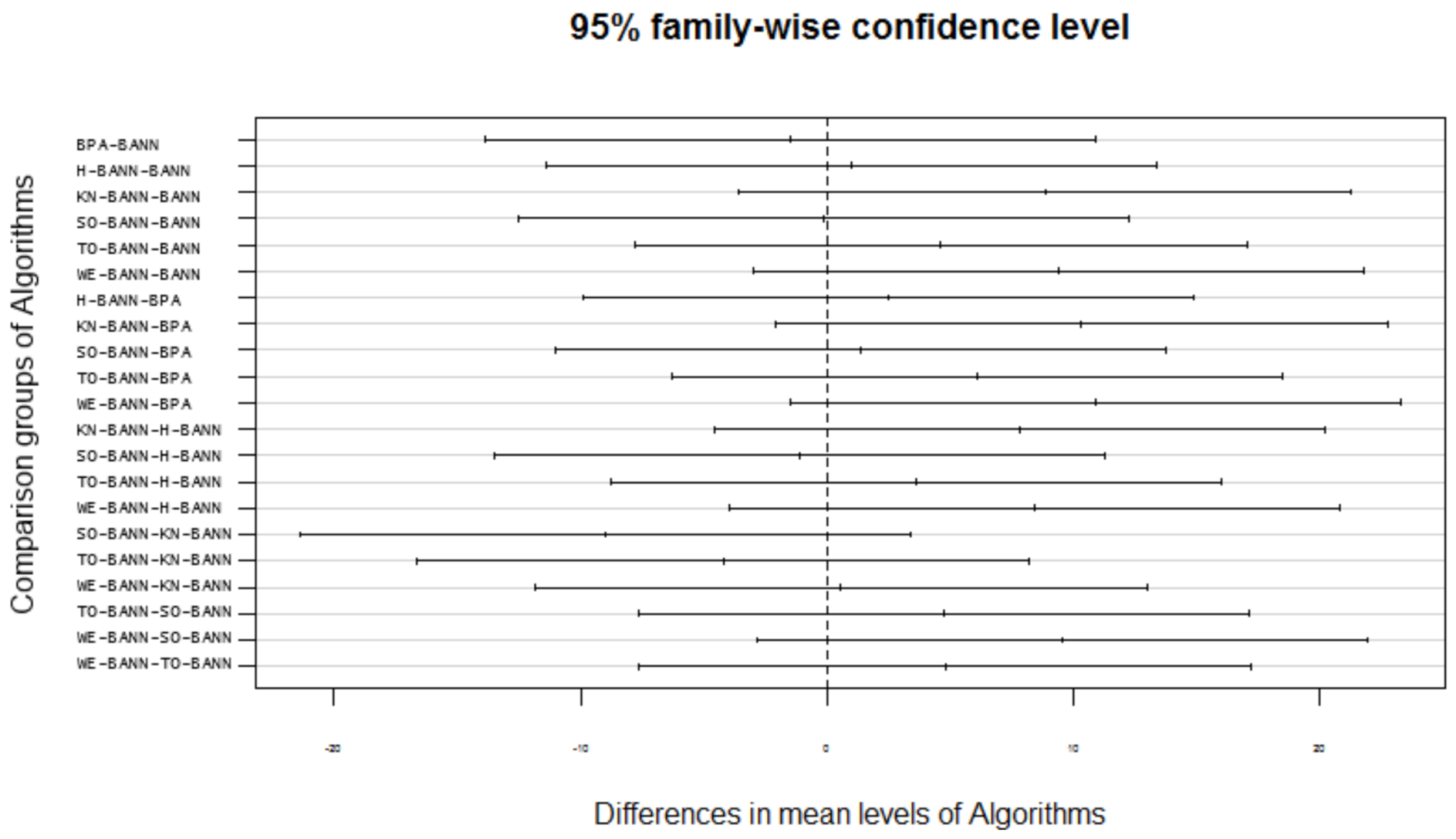
Figure 63.
Multi-comparison post-hoc Tukey test graph of all BA-based.
Figure 63.
Multi-comparison post-hoc Tukey test graph of all BA-based.
Table 1.
Experimental setting of parameters.
Table 1.
Experimental setting of parameters.
| Parameter | Value | | |
|---|
| Search Space | [100, −100] | | |
| Dimensions | 10 | 20 | 30 |
| Iterations | 1000 | 2000 | 3000 |
| Population size | 50 | | |
| Number of PSO Runs | 10 | | |
Table 2.
Parameters setting of parameters.
Table 2.
Parameters setting of parameters.
| Algorithm | Parameters |
|---|
| PSO | c1=c2=1.49, w = linearly decreasing |
| BA | =40, , |
| DE | F ∈ [0.4, 1], CR ∈ 0.6 |
Table 3.
Function table with characteristics.
Table 3.
Function table with characteristics.
| Sr.# | Function Name | Objective Function | Search Space | Optimal Value |
|---|
| 01 | Sphere | | | 0 |
| 02 | Rastrigin | | | 0 |
| 03 | Axis parallel hyper-ellipsoid | | | 0 |
| 04 | Rotated hyper ellipsoid | | | 0 |
| 05 | Moved Axis | | | 0 |
| 06 | Sum of different power | | | 0 |
| 07 | ChungReynolds | | | 0 |
| 08 | Csendes | | | 0 |
| 09 | Schaffer | | | 0 |
| 10 | Schumer_Steiglitz | | | 0 |
| 11 | Schwefel | | | 0 |
| 12 | Schwefel1.2 | | | 0 |
| 13 | Schwefel 2.21 | | | 0 |
| 14 | Schwefel 2.22 | | | 0 |
| 15 | Schwefel 2.23 | | | 0 |
| 16 | Zakharov | | | 0 |
Table 4.
Comparative results for all PSO-based approaches on 16 standard benchmark functions.
Table 4.
Comparative results for all PSO-based approaches on 16 standard benchmark functions.
| Functions | DIM × Itr | PSO | SO−PSO | H−PSO | TO−PSO | WE−PSO | KN−PSO |
|---|
| Mean | Mean | Mean | Mean | Mean | Mean |
|---|
| F1 | 10 × 1000 | 2.33 × 10−74 | 2.74 × 10−76 | 3.10 × 10−77 | 5.57 × 10−78 | 5.91 × 10−78 | 0.0000 × 10+00 |
| 20 × 2000 | 1.02 × 10−84 | 8.20 × 10−88 | 1.76 × 10−90 | 1.30 × 10−90 | 4.95 × 10−90 | 3.14001 × 10−217 |
| 30 × 3000 | 1.77 × 10⁻²⁶ | 7.67 × 10⁻²⁰ | 4.13 × 10⁻³² | 1.25 × 10−51 | 1.30 × 10−42 | 8.91595 × 10−88 |
| F2 | 10 × 1000 | 4.97 × 10−01 | 4.97 × 10−01 | 7.96 × 10−01 | 3.98 × 10−01 | 2.98 × 10−01 | −8602.02 |
| 20 × 2000 | 8.17 × 10+00 | 6.47 × 10+00 | 3.58 × 10+00 | 2.89 × 10+00 | 3.11 × 10+00 | −31,433.3 |
| 30 × 3000 | 1.01 × 10+01 | 9.86 × 10+00 | 9.45 × 10+00 | 8.16 × 10+00 | 7.76 × 10+00 | −60,711.8 |
| F3 | 10 × 1000 | 8.70 × 10−80 | 1.79 × 10−79 | 4.87 × 10−79 | 3.91 × 10−82 | 4.40 × 10−81 | 0.0000 × 10+00 |
| 20 × 2000 | 2.62144 | 7.86432 | 2.62144 | 7.07 × 10−90 | 1.78 × 10−89 | 4.78718 × 10−237 |
| 30 × 3000 | 2.62 × 10+01 | 1.57 × 10+01 | 1.05 × 10+01 | 7.70 × 10⁻³⁵ | 3.87 × 10−57 | 1.57084 × 10−97 |
| F4 | 10 × 1000 | 4.46 × 10−147 | 3.86 × 10−147 | 9.78 × 10−145 | 7.29 × 10−148 | 1.24 × 10−150 | 0.0000 × 10+00 |
| 20 × 2000 | 3.14 × 10−155 | 9.27 × 10−154 | 2.75 × 10−159 | 5.14 × 10−158 | 4.96 × 10−159 | 0.0000 × 10+00 |
| 30 × 3000 | 1.82 × 10−133 | 2.36 × 10−135 | 8.53 × 10−130 | 3.13 × 10−138 | 2.54 × 10−136 | 1.6439 × 10−228 |
| F5 | 10 × 1000 | 4.35 × 10−79 | 8.95 × 10−79 | 2.43 × 10−78 | 2.04 × 10−80 | 2.20 × 10−80 | 0.0000 × 10+00 |
| 20 × 2000 | 1.31 × 10+01 | 3.93 × 10+01 | 1.31 × 10+01 | 3.54 × 10−89 | 3.12 × 10−89 | 2.39359 × 10−236 |
| 30 × 3000 | 1.31 × 10+02 | 7.86 × 10+01 | 5.24 × 10+01 | 3.85 × 10⁻³⁴ | 1.94 × 10−56 | 2.9093 × 10−87 |
| F6 | 10 × 1000 | 1.70 × 10−61 | 4.45 × 10−64 | 7.29 × 10−66 | 2.46 × 10−66 | 4.62 × 10−66 | 3.04226 × 10−318 |
| 20 × 2000 | 3.25 × 10−112 | 4.39 × 10−112 | 5.01 × 10−109 | 2.56 × 10−115 | 4.45 × 10−113 | 8.59557 × 10−277 |
| 30 × 3000 | 7.21 × 10−135 | 4.10 × 10−124 | 1.51 × 10−134 | 6.22×10−137 | 6.96 × 10−135 | 2.33033 × 10−223 |
| F7 | 10 × 1000 | 2.96 × 10−157 | 2.39 × 10−157 | 1.28 × 10−157 | 4.89 × 10−159 | 2.47 × 10−163 | 0.0000 × 10+00 |
| 20 × 2000 | 8.79 × 10−177 | 1.77 × 10−184 | 3.49 × 10−183 | 3.09 × 10−187 | 3.41 × 10−186 | 0.0000 × 10+00 |
| 30 × 3000 | 1.23 × 10−82 | 1.25 × 10−116 | 5.99 × 10−130 | 5.01 × 10−135 | 4.60 × 10−134 | 8.03288 × 10−175 |
| F8 | 10 × 1000 | 4.39 × 10−200 | 1.98 × 10−194 | 4.51 × 10−197 | 1.26 × 10−202 | 8.99 × 10−201 | 4.9228 × 10−67 |
| 20 × 2000 | 1.57 × 10⁻²⁰ | 1.04 × 10−93 | 1.10 × 10−148 | 2.84 × 10−157 | 4.09 × 10−151 | 4.5887 × 10⁻¹⁶ |
| 30 × 3000 | 1.89 × 10−09 | 4.54 × 10⁻¹⁰ | 1.14 × 10−08 | 1.40 × 10⁻¹⁰ | 1.34 × 10−09 | 2.2334 × 10−08 |
| F9 | 10 × 1000 | 5.49 × 10−01 | 1.30 × 10−01 | 2.02 × 10−01 | 1.26 × 10−01 | 1.42 × 10−01 | 0.824968 |
| 20 × 2000 | 2.05 × 10+00 | 7.83 × 10−01 | 6.83 × 10−01 | 5.84 × 10−01 | 4.32 × 10−01 | 4.56265 |
| 30 × 3000 | 1.12 × 10+00 | 9.99 × 10−01 | 9.56 × 10−01 | 9.06 × 10−01 | 9.12 × 10−01 | 7.25675 |
| F10 | 10 × 1000 | 2.23 × 10−138 | 2.23 × 10−138 | 4.35 × 10−137 | 1.02 × 10−140 | 1.10 × 10−139 | 0.0000 × 10+00 |
| 20 × 2000 | 3.79 × 10−148 | 7.87 × 10−149 | 4.19 × 10−147 | 3.78 × 10−151 | 8.73 × 10−153 | 0.0000 × 10+00 |
| 30 × 3000 | 4.43 × 10−126 | 7.52 × 10−133 | 1.57 × 10−128 | 2.03 × 10−134 | 1.38 × 10−133 | 2.26229 × 10−221 |
| F11 | 10 × 1000 | 3.75 × 10−187 | 1.57 × 10−192 | 2.15 × 10−191 | 5.57 × 10−198 | 8.99 × 10−198 | 0.0000 × 10+00 |
| 20 × 2000 | 5.29 × 10−193 | 2.53 × 10−195 | 8.45 × 10−195 | 8.45 × 10−195 | 9.83 × 10−197 | 0.0000 × 10+00 |
| 30 × 3000 | 4.82 × 10−154 | 8.84 × 10−159 | 5.49 × 10−168 | 2.04 × 10−170 | 5.75 × 10−173 | 9.00586 × 10−278 |
| F12 | 10 × 1000 | 1.13 × 10−01 | 1.67 × 10−02 | 2.28 × 10−02 | 4.78 × 10−03 | 2.89 × 10−03 | 2.739 × 10⁻¹² |
| 20 × 2000 | 1.39 × 10+01 | 5.03 × 10+00 | 2.95 × 10+00 | 1.28 × 10+00 | 1.67 × 10+00 | 7.819 × 10+00 |
| 30 × 3000 | 7.45 × 10+00 | 1.22 × 10+01 | 8.74 × 10+00 | 2.94 × 10+00 | 4.94 × 10+00 | 2.239 × 10+01 |
| F13 | 10 × 1000 | 8.04 × 10⁻²⁶ | 8.01 × 10⁻²⁷ | 3.59 × 10⁻²⁷ | 1.24 × 10⁻²⁷ | 1.41 × 10⁻²⁷ | 0.0000 × 10+00 |
| 20 × 2000 | 1.42 × 10−08 | 2.64 × 10⁻¹¹ | 3.29 × 10⁻¹⁰ | 2.99 × 10⁻¹⁰ | 2.14 × 10⁻¹² | 0.0000 × 10+00 |
| 30 × 3000 | 6.20 × 10−03 | 1.41 × 10−03 | 9.36 × 10−03 | 1.12 × 10−03 | 1.41 × 10−03 | 0.0000 × 10+00 |
| F14 | 10 × 1000 | 3.62 × 10−38 | 3.62 × 10−38 | 5.92 × 10−36 | 6.92 × 10−39 | 1.95 × 10−38 | 7.78286 × 10−197 |
| 20 × 2000 | 6.27 × 10⁻¹⁰ | 1.38 × 10−09 | 7.91 × 10⁻¹³ | 2.49 × 10⁻¹² | 1.17 × 10⁻¹³ | 6.6163 × 10⁻¹² |
| 30 × 3000 | 2.56 × 10−06 | 4.80 × 10+01 | 1.34 × 10−06 | 5.40 × 10⁻¹¹ | 4.88 × 10−09 | 9.3032 × 10−06 |
| F15 | 10 × 1000 | 1.10 × 10−294 | 3.19 × 10−301 | 2.78 × 10−307 | 1.94 × 10−307 | 3.21 × 10−308 | 6.26612 × 10−138 |
| 20 × 2000 | 6.16 × 10−271 | 5.09 × 10−276 | 3.74 × 10−270 | 1.60 × 10−276 | 4.85 × 10−268 | 1.29033 × 10⁻²⁵ |
| 30 × 3000 | 3.08 × 10−207 | 1.04 × 10−200 | 8.12 × 10−209 | 2.34 × 10−215 | 3.06 × 10−212 | 2.27 × 10−06 |
| F16 | 10 × 1000 | 5.4835385 | 8.5299 × 10 | 3.3074 × 10⁻¹⁶ | 1.224803 | 8.3354 × 10−07 | 2.26476 × 10⁻²⁷ |
| 20 × 2000 | 83.467 | 1.6344 | 0.18037 | 49.16841 | 5.1322 | 7.17014 × 10−72 |
| 30 × 3000 | 265.90708 | 282.1864 | 45.0408 | 133.9679 | 67.0301 | 5.45179 × 10−251 |
Table 5.
Mean ranks obtained by Kruskal–Wallis and Friedman tests for all.
Table 5.
Mean ranks obtained by Kruskal–Wallis and Friedman tests for all.
| Approaches | Friedman Value | p-Value | Kruskal–Wallis | p-Value |
|---|
| PSO | 39.09 | 0.001 | 39.33 | 0.001 |
| SO-PSO | 37.47 | 0.001 | 38.39 | 0.001 |
| H-PSO | 38.50 | 0.001 | 38.91 | 0.001 |
| TO-PSO | 41.79 | 0.000 | 42.67 | 0.000 |
| WE-PSO | 41.88 | 0.000 | 42.50 | 0.000 |
| KN-PSO | 18.24 | 0.001 | 23.31 | 0.002 |
Table 6.
Comparative results for all DE-based approaches on 16 standard benchmark functions.
Table 6.
Comparative results for all DE-based approaches on 16 standard benchmark functions.
| Functions | DIM × Iter | DE | DE−H | DE−S | DE−TO | DE−WE | DE−KN |
|---|
| F1 | 10 × 1000 | 1.1464 × 10−44 | 2.1338 × 10−44 | 5.8561 × 10−44 | 7.4117 × 10−45 | 7.4827 × 10−39 | 5.7658 × 10−39 |
| 20 × 2000 | 3.3550 × 10−46 | 7.2338 × 10−46 | 1.3545 × 10−45 | 1.2426 × 10−45 | 9.6318 × 10−45 | 7.1501 × 10−45 |
| 30 × 3000 | 8.8946 × 10−47 | 1.2273 × 10−45 | 9.4228 × 10−46 | 1.6213 × 10−46 | 6.2007 × 10−46 | 5.7425 × 10−46 |
| F2 | 10 × 1000 | 0.0000 × 10+00 | 0.0000 × 10+00 | 0.0000 × 10+00 | 0.0000 × 10+00 | 0.0000 × 10+00 | 0.0000 × 10+00 |
| 20 × 2000 | 0.0000 × 10+00 | 0.0000 × 10+00 | 0.0000 × 10+00 | 0.0000 × 10+00 | 0.0000 × 10+00 | 0.0000 × 10+00 |
| 30 × 3000 | 1.8392 × 10+01 | 1.1846 × 10+01 | 1.8871 × 10+01 | 3.7132 × 10−01 | 5.0821 × 10+00 | 6.6313 × 10+00 |
| F3 | 10 × 1000 | 5.00325 × 10−44 | 1.5019 × 10−38 | 9.3956 × 10−44 | 4.7807 × 10−44 | 1.6251 × 10−38 | 1.3411 × 10−38 |
| 20 × 2000 | 2.56987 × 10−45 | 4.1485 × 10−44 | 1.5339 × 10−44 | 3.0262 × 10−45 | 9.5984 × 10−44 | 1.3606 × 10−43 |
| 30 × 3000 | 1.01692 × 10−45 | 2.7349 × 10−45 | 4.0581 × 10−45 | 4.5726 ×10−45 | 4.5686 × 10−45 | 5.4659 × 10−45 |
| F4 | 10 × 1000 | 5.81825 × 10−42 | 3.0950 × 10−36 | 2.2300 × 10−41 | 1.6903 × 10−41 | 1.1331 × 10−36 | 3.8869 × 10−36 |
| 20 × 2000 | 2.70747 × 10−43 | 1.0658 × 10−41 | 1.6730 × 10−42 | 1.3490 × 10−42 | 1.3094 × 10−41 | 6.0053 × 10−42 |
| 30 × 3000 | 2.99887 × 10−43 | 1.4032 × 10−42 | 4.4442 × 10−42 | 5.9186 × 10−43 | 4.6922 × 10−43 | 1.4829 × 10−42 |
| F5 | 10 × 1000 | 1.65318 × 10−43 | 4.7939 × 10−38 | 7.0329 × 10−43 | 4.8106 × 10−43 | 4.3219 × 10−38 | 3.5770 × 10−38 |
| 20 × 2000 | 1.39082 × 10−44 | 3.6325 × 10−43 | 4.2191 × 10−44 | 2.7448 × 10−44 | 5.8557 × 10−43 | 1.4008 × 10−43 |
| 30 × 3000 | 6.07162 × 10−45 | 1.7557 × 10−44 | 1.6295 × 10−44 | 2.0582 × 10−44 | 8.6773 × 10−45 | 4.2285 × 10−44 |
| F6 | 10 × 1000 | 7.8201 × 10−96 | 3.8819 × 10−96 | 9.7956 × 10−96 | 2.3292 × 10−95 | 8.4774 × 10−94 | 2.8037 × 10−95 |
| 20 × 2000 | 1.6847 × 10−125 | 8.6880 × 10−124 | 5.9005 × 10−122 | 8.7800 × 10−123 | 3.7438 × 10−124 | 1.3947 × 10−124 |
| 30 × 3000 | 2.4533 × 10−140 | 1.5487 × 10−139 | 5.7211 × 10−138 | 4.4492 × 10−137 | 6.5749 × 10−140 | 3.4442 × 10−137 |
| F7 | 10 × 1000 | 8.0217 × 10−75 | 7.3243 × 10−67 | 5.7807 × 10−66 | 1.0243 × 10−73 | 1.9035 × 10−67 | 1.4359 × 10−65 |
| 20 × 2000 | 4.0682 × 10−71 | 1.5037 × 10−70 | 1.5747 × 10−69 | 1.0623 × 10−70 | 5.5546 × 10−70 | 2.3507 × 10−70 |
| 30 × 3000 | 8.5895 × 10−68 | 6.6009 × 10−68 | 3.3919 × 10−67 | 2.6036 × 10−67 | 1.1587 × 10−67 | 2.1901 × 10−67 |
| F8 | 10 × 1000 | 7.0221 × 10−120 | 3.4271 × 10−108 | 2.7718 × 10−108 | 6.3092 × 10−118 | 3.9423 × 10−106 | 9.9394 × 10−108 |
| 20 × 2000 | 5.2096 × 10−108 | 7.7158 × 10−89 | 1.4732 × 10−106 | 8.8720 × 10−107 | 3.4490 × 10−107 | 2.2539 × 10−106 |
| 30 × 3000 | 1.2538 × 10−98 | 1.8071 × 10−98 | 1.1085 × 10−95 | 7.2462 × 10−98 | 2.5375 × 10−99 | 5.8040 × 10−98 |
| F9 | 10 × 1000 | 0.0000 × 10+00 | 0.0000 × 10+00 | 0.0000 × 10+00 | 0.0000 × 10+00 | 0.0000 × 10+00 | 0.0000 × 10+00 |
| 20 × 2000 | 0.0000 × 10+00 | 0.0000 × 10+00 | 0.0000 × 10+00 | 0.0000 × 10+00 | 0.0000 × 10+00 | 0.0000 × 10+00 |
| 30 × 3000 | 0.0000 × 10+00 | 0.0000 × 10+00 | 0.0000 × 10+00 | 0.0000 × 10+00 | 0.0000 × 10+00 | 0.0000 × 10+00 |
| F10 | 10 × 1000 | 1.3459 × 10−75 | 2.6493 × 10−66 | 2.6884 × 10−66 | 3.6168 × 10−67 | 3.8397 × 10−67 | 1.8408 × 10−66 |
| 20 × 2000 | 3.0478 × 10−71 | 1.6106 × 10−69 | 5.5253 × 10−69 | 2.7746 × 10−70 | 5.3662 × 10−70 | 5.0931 × 10−70 |
| 30 × 3000 | 8.2514 × 10−68 | 1.0937 × 10−66 | 4.1120 × 10−67 | 1.3055 × 10−67 | 3.5397 × 10−68 | 6.073 × 10−67 |
| F11 | 10 × 1000 | 2.3417 × 10−42 | 1.2483 × 10−41 | 1.3726 × 10−41 | 6.3337 × 10−42 | 4.8161 × 10−42 | 7.34640 × 10−42 |
| 20 × 2000 | 8.4769 × 10−44 | 3.5140 × 10−43 | 3.3777 × 10−43 | 2.4721 × 10−43 | 1.9553 × 10−43 | 3.6961 × 10−43 |
| 30 × 3000 | 3.6888 × 10−44 | 6.9938 × 10−44 | 2.5123 × 10−43 | 1.4710 × 10−43 | 4.0019 × 10−44 | 3.9503 × 10−43 |
| F12 | 10 × 1000 | 2.3304 × 10+00 | 4.4354 × 10+00 | 3.4520 × 10+00 | 5.1229 × 10+00 | 3.8782 × 10+00 | 2.7840 × 10+00 |
| 20 × 2000 | 3.1768 × 10+04 | 3.9596 × 10+04 | 3.8814 × 10+04 | 2.9488 × 10+04 | 4.1181 × 10+04 | 4.0914 × 10+04 |
| 30 × 3000 | 1.1760 × 10+06 | 1.0300 × 10+06 | 1.3402 × 10+06 | 1.2008 × 10+06 | 1.0916 × 10+06 | 1.0160 × 10+06 |
| F13 | 10 × 1000 | 1.3940 × 10−65 | 1.3756 × 10−64 | 3.1956 × 10−66 | 9.3609 × 10−64 | 5.4864 × 10−63 | 9.2695 × 10−63 |
| 20 × 2000 | 2.0163 × 10−111 | 8.5333 × 10−110 | 8.5260 × 10−111 | 3.9836 × 10−109 | 5.0102 × 10−115 | 4.4624 × 10−110 |
| 30 × 3000 | 1.4146 × 10−156 | 4.3434 × 10−156 | 4.4702 × 10−154 | 4.3862 × 10−151 | 1.0781 × 10−153 | 1.0142 × 10−149 |
| F14 | 10 × 1000 | 9.1259 × 10⁻²⁴ | 2.1900 × 10⁻²³ | 2.5559 × 10⁻²³ | 2.9039 × 10⁻²³ | 1.9174 × 10⁻²³ | 3.3427 × 10⁻²³ |
| 20 × 2000 | 2.6867 × 10⁻²⁵ | 3.8631 × 10⁻²⁵ | 1.5177 × 10⁻²⁴ | 5.5714 × 10⁻²⁵ | 4.5049 × 10⁻²⁵ | 5.6503 × 10⁻²⁵ |
| 30 × 3000 | 5.9241 × 10⁻²⁶ | 8.6401 × 10⁻²⁶ | 8.4348 × 10⁻²⁶ | 1.4630 × 10⁻²⁵ | 9.7932 × 10⁻²⁶ | 1.4921 × 10⁻²⁵ |
| F15 | 10 × 1000 | 1.0493 × 10−185 | 4.0276 × 10−181 | 5.0331 × 10−182 | 3.1770 × 10−183 | 1.1698 × 10−180 | 2.6563 × 10−182 |
| 20 × 2000 | 2.9407 × 10−159 | 9.9152 × 10−159 | 2.1401 × 10−158 | 9.0345 × 10−156 | 3.8871 × 10−158 | 8.0144 × 10−160 |
| 30 × 3000 | 4.6769 × 10−138 | 1.0737 × 10−137 | 7.0544 × 10−138 | 8.0376 × 10−138 | 4.9091 × 10−139 | 1.1054 × 10−137 |
| F16 | 10 × 1000 | 1.8635 × 10−04 | 1.8109 × 10−02 | 4.9798 × 10−02 | 5.8605 × 10−04 | 1.4858 × 10−02 | 3.7220 × 10−02 |
| 20 × 2000 | 1.1032 × 10+00 | 1.6605 × 10+00 | 1.7157 × 10+00 | 1.4875 × 10+00 | 1.5697 × 10+00 | 1.2008 × 10+00 |
| 30 × 3000 | 2.8283 × 10+01 | 2.2049 × 10+01 | 2.9388 × 10+01 | 2.8205 × 10+01 | 2.5794 × 10+01 | 2.9526 × 10+01 |
Table 7.
Mean ranks obtained by Kruskal–Wallis and Friedman tests for all.
Table 7.
Mean ranks obtained by Kruskal–Wallis and Friedman tests for all.
| Approaches | Friedman Value | p-Value | Kruskal–Wallis | p-Value |
|---|
| DE | 63.74 | 0.000 | 65.11 | 0.000 |
| DE-H | 59.31 | 0.000 | 60.41 | 0.000 |
| DE-S | 64.01 | 0.000 | 65.05 | 0.000 |
| DE-TO | 63.76 | 0.000 | 65.35 | 0.000 |
| DE-WE | 63.35 | 0.000 | 63.93 | 0.000 |
| DE-KN | 63.33 | 0.000 | 64.06 | 0.000 |
Table 8.
Comparative results for all BA-based approaches on 16 standard benchmark functions.
Table 8.
Comparative results for all BA-based approaches on 16 standard benchmark functions.
| | | BA | BA−SO | BA−HA | BA−TO | BA−WE | BA−KN |
|---|
| F# | DIM × Iter | Mean | Mean | Mean | Mean | Mean | Mean |
|---|
| F1 | 10 × 1000 | 1.59 × 10−07 | 1.03 × 10−07 | 1.32 × 10−07 | 8.95 × 10−08 | 0.63202 | 0.88186 |
| 20 × 2000 | 1.02 × 10−84 | 8.20 × 10−88 | 1.76 × 10−90 | 1.30 × 10−90 | 4.95 × 10−90 | 3.14001 × 10−217 |
| 30 × 3000 | 1.77 × 10⁻²⁶ | 7.67 × 10⁻²⁰ | 4.13 × 10⁻³² | 1.25 × 10−51 | 1.30 × 10−42 | 8.91595 × 10−88 |
| F2 | 10 × 1000 | 4.13 × 10+01 | 3.17 × 10+01 | 1.82 × 10+01 | 3.55 × 10+01 | 37.9883 | 40.8852 |
| 20 × 2000 | 1.06 × 10+02 | 5.78 × 10+01 | 1.15 × 10+02 | 9.47 × 10+01 | 140.2023 | 147.8938 |
| 30 × 3000 | 2.05 × 10+02 | 1.46 × 10+02 | 1.83 × 10+02 | 1.69 × 10+02 | 271.307 | 275.8626 |
| F3 | 10 × 1000 | 5.93 × 10−07 | 4.70 × 10−07 | 3.99 × 10−07 | 4.0 × 10−07 | 2.9125 | 5.2009 |
| 20 × 2000 | 1.57 × 10−06 | 1.05 × 10−06 | 1.29 × 10−06 | 1.05 × 10−06 | 49.3011 | 72.4834 |
| 30 × 3000 | 3.53 × 10−06 | 3.48 × 10−06 | 3.27 × 10−06 | 2.20 × 10−06 | 197.4826 | 257.9855 |
| F4 | 10 × 1000 | 2.19 × 10+05 | 1.11 × 10+05 | 1.66 × 10⁻¹⁴ | 2.07 × 10+02 | 9.268 | 13.5548 |
| 20 × 2000 | 2.56 × 10+07 | 2.42 × 10+07 | 2.31 × 10+07 | 1.50 × 10+07 | 160.0394 | 255.3367 |
| 30 × 3000 | 1.43 × 10+08 | 1.38 × 10+08 | 3.30 × 10+08 | 1.34 × 10+08 | 656.5592 | 946.3934 |
| F5 | 10 × 1000 | 2.81 × 10−06 | 2.67 × 10−06 | 1.69 × 10−06 | 2.47 × 10−06 | 19.7651 | 22.0461 |
| 20 × 2000 | 7.43 × 10−06 | 5.77 × 10−06 | 6.25 × 10−06 | 5.33 × 10−06 | 250.8679 | 293.7174 |
| 30 × 3000 | 1.59 × 10−05 | 1.43 × 10−05 | 1.50 × 10−05 | 9.59 × 10−06 | 1029.0595 | 1277.0077 |
| F6 | 10 × 1000 | 6.19 × 10−04 | 4.54 × 10−04 | 3.89 × 10−04 | 3.39 × 10−04 | 10.1173 | 10.1222 |
| 20 × 2000 | 7.96 × 10−04 | 6.32 × 10−04 | 7.77 × 10−04 | 5.78 × 10−04 | 20.2119 | 20.1467 |
| 30 × 3000 | 1.05 × 10−03 | 1.01 × 10−03 | 1.01 × 10−03 | 6.65 × 10−04 | 30.3623 | 30.2845 |
| F7 | 10 × 1000 | 15.8966 | 18.851 | 18.2544 | 15.3465 | 16.9429 | 18.4835 |
| 20 × 2000 | 839.1846 | 686.8456 | 762.1919 | 690.0657 | 876.2518 | 496.7506 |
| 30 × 3000 | 4892.6864 | 4877.7072 | 4476.0152 | 4482.3035 | 5361.4808 | 3860.4327 |
| F8 | 10 × 1000 | 0.023455 | 0.01557 | 0.018152 | 0.016735 | 0.024264 | 0.020123 |
| 20 × 2000 | 0.45222 | 0.44101 | 0.39478 | 0.39719 | 0.39445 | 0.24522 |
| 30 × 3000 | 1.7266 | 1.0969 | 1.3512 | 1.3717 | 1.4375 | 0.99905 |
| F9 | 10 × 1000 | 4.1394 | 3.8003 | 3.8687 | 4.0739 | 3.4024 | 3.9516 |
| 20 × 2000 | 8.587 | 8.8019 | 8.5686 | 8.585 | 8.8319 | 8.5709 |
| 30 × 3000 | 13.0878 | 13.502 | 13.4188 | 13.2291 | 13.2835 | 13.4514 |
| F10 | 10 × 1000 | 6.66 × 10⁻¹⁵ | 3.31 × 10⁻¹⁵ | 1.90 × 10⁻¹⁵ | 2.43 × 10⁻¹⁵ | 1.3357 | 2.0298 |
| 20 × 2000 | 3.65 × 10⁻¹⁵ | 2.03 × 10⁻¹⁵ | 1.55 × 10⁻¹⁵ | 1.12 × 10⁻¹⁵ | 24.9415 | 53.16 |
| 30 × 3000 | 1.71 × 10⁻¹⁵ | 1.06 × 10⁻¹⁵ | 1.06 × 10⁻¹⁵ | 9.24 × 10⁻¹⁶ | 115.9262 | 318.7949 |
| F11 | 10 × 1000 | 218.1498 | 113.8805 | 105.5027 | 58.8987 | 69.5656 | 52.7079 |
| 20 × 2000 | 31293.8096 | 17609.1493 | 20760.6498 | 17638.3139 | 26832.6985 | 13990.4835 |
| 30 × 3000 | 651165.7416 | 338621.8857 | 323118.6791 | 268752.5102 | 432441.3838 | 213235.6129 |
| F12 | 10 × 1000 | 2.96 × 10+03 | 2.21 × 10+03 | 2.27 × 10+03 | 1.49 × 10+03 | 253.722 | 272.7033 |
| 20 × 2000 | 2.21 × 10+04 | 1.28 × 10+04 | 1.49 × 10+04 | 5.93 × 10+03 | 11265.9616 | 9512.9456 |
| 30 × 3000 | 2.65 × 10+05 | 7.06 × 10+04 | 1.65 × 10+05 | 7.19 × 10+04 | 71723.2776 | 67828.8796 |
| F13 | 10 × 1000 | 1.4453 | 1.2827 | 1.2766 | 1.298 | 1.3884 | 1.3271 |
| 20 × 2000 | 2.7303 | 2.8404 | 2.746 | 2.7973 | 2.9688 | 2.6632 |
| 30 × 3000 | 3.9975 | 3.9993 | 4.2588 | 4.0509 | 4.2646 | 3.9435 |
| F14 | 10 × 1000 | 3.83 × 10+06 | 7.39 × 10+06 | 2.33 × 10+05 | 2.69 × 10+04 | 4.71 × 10+08 | 4.23 × 10+08 |
| 20 × 2000 | 7.28 × 10+19 | 1.55 × 10+17 | 1.30 × 10+20 | 1.69 × 10+18 | 7.78 × 10+19 | 2.94 × 10+19 |
| 30 × 3000 | 5.15 × 10+33 | 3.30 × 10+31 | 8.00 × 10+32 | 1.21 × 10+30 | 1.99 × 10+33 | 5.50 × 10+33 |
| F15 | 10 × 1000 | 2.40 × 10−36 | 1.11 × 10−37 | 2.08 × 10−37 | 2.19 × 10−37 | 5.27 × 10−02 | 3.76 × 10−02 |
| 20 × 2000 | 1.50 × 10−37 | 4.91 × 10−38 | 5.70 × 10−38 | 4.72 × 10−39 | 1.83 × 10+02 | 1.30 × 10+02 |
| 30 × 3000 | 1.39 × 10−37 | 2.20 × 10−38 | 7.43 × 10−38 | 1.15 × 10−38 | 1.08 × 10+04 | 2.04 × 10+04 |
| F16 | 10 × 1000 | 4.3197 | 3.2767 | 3.0513 | 2.8833 | 4.0923 | 3.0495 |
| 20 × 2000 | 21.9881 | 24.5093 | 22.608 | 2.8833 | 23.917 | 22.102 |
| 30 × 3000 | 89.0053 | 80.3004 | 74.4391 | 66.7812 | 67.7061 | 63.0376 |
Table 9.
Mean ranks obtained by Kruskal–Wallis and Friedman tests for all.
Table 9.
Mean ranks obtained by Kruskal–Wallis and Friedman tests for all.
| Approaches | Friedman Value | p-Value | Kruskal–Wallis | p-Value |
|---|
| BA | 44.88 | 0.000 | 46.15 | 0.000 |
| BA-SO | 44.82 | 0.000 | 46.00 | 0.000 |
| BA-HA | 40.29 | 0.000 | 40.90 | 0.000 |
| BA-TO | 44.71 | 0.000 | 45.16 | 0.000 |
| BA-WE | 40.12 | 0.001 | 32.67 | 0.005 |
| BA-KN | 39.53 | 0.000 | 32.32 | 0.006 |
Table 10.
Characteristics of UCI benchmarks DataSets.
Table 10.
Characteristics of UCI benchmarks DataSets.
| S. No | Data Set | Continuous | Nature | No. of Inputs | No. of Classes |
|---|
| 1 | Diabetes | 8 | Real | 8 | 2 |
| 2 | Heart | 13 | Real | 13 | 2 |
| 3 | Wine | 13 | Real | 13 | 3 |
| 4 | Seed | 7 | Real | 7 | 3 |
| 5 | Vertebral | 6 | Real | 6 | 2 |
| 6 | Blood Tissue | 5 | Real | 5 | 2 |
| 7 | Memo Graphy | 6 | Real | 6 | 2 |
Table 11.
Results of 10-fold classification rates of ANN-training methods in 7 datasets for accuracy.
Table 11.
Results of 10-fold classification rates of ANN-training methods in 7 datasets for accuracy.
| S. No | Data Sets | Type | BPA | PSONN | SO-PSONN | H-PSONN | TO-PSONN | WE-PSONN | KN-PSONN |
|---|
| Ts. Acc | Ts. Acc | Ts. Acc | Ts. Acc | Ts. Acc | Ts. Acc | Ts. Acc |
|---|
| 1 | Diabetes | 2-Class | 65.3% | 69.1% | 69.1% | 71.6% | 73.3% | 74.1% | 78.5% |
| 2 | Heart | 2-Class | 68.3% | 72.5% | 67.5% | 72.5% | 77.5 | 77.5% | 79% |
| 3 | Wine | 3-Class | 62.17% | 61.11% | 66.66% | 67.44% | 69.44% | 69.6% | 72% |
| 4 | Seed | 3-Class | 70.56% | 77.77% | 84.44% | 77.77% | 88.88% | 91.11% | 93% |
| 5 | Vertebral | 2-Class | 84.95% | 92.85% | 92.85% | 92.85% | 94.64% | 94.64% | 96% |
| 6 | Blood Tissue | 2-Class | 73.47% | 78.6% | 78.66% | 70% | 82.66% | 84% | 87% |
| 7 | Memo Graphy | 2-Class | 71.26% | 76.66% | 63% | 85% | 88.88% | 96.66% | 98% |
Table 12.
One-way ANOVA results of PSO variants.
Table 12.
One-way ANOVA results of PSO variants.
| Parameter | Relation | Sum of Squares | df | Mean Square | F | Significance |
|---|
| Testing Accuracy | Among groups | 1318.2 | 6 | 219.697 | 2.3676 | 0.04639 |
Table 13.
Results of 10-fold classification rates of ANN-training methods in 7 datasets for accuracy.
Table 13.
Results of 10-fold classification rates of ANN-training methods in 7 datasets for accuracy.
| S. No | Data Sets | Type | BPA | DENN | SO-DENN | H-DENN | TO-DENN | KN-DENN | WE-DENN |
|---|
| Ts. Acc | Ts. Acc | Ts. Acc | Ts. Acc | Ts. Acc | Ts. Acc | Ts. Acc |
|---|
| 2 | Diabetes | 2-Class | 65.3% | 66.1% | 68.16% | 69.6% | 71.30% | 67.17% | 75.50% |
| 3 | Heart | 2-Class | 68.3% | 70.5% | 72.5% | 71.5% | 74.50% | 72.56% | 76.34% |
| 4 | Wine | 3-Class | 62.17% | 64.7% | 65.19% | 66.20% | 66.59% | 68.25% | 70.51% |
| 5 | Seed | 3-Class | 70.56% | 75.16% | 75.29% | 75.77% | 82.13% | 86.76% | 91.54% |
| 6 | Vertebral | 2-Class | 84.95% | 87.13% | 89.26% | 91.15% | 93.64% | 90.17% | 96.25% |
| 7 | Blood Tissue | 2-Class | 73.47% | 76.23% | 74.16% | 72..21% | 84.76% | 81.34% | 86.45% |
| 9 | Memo Graphy | 2-Class | 71.26% | 74.39% | 68.37% | 82.45% | 86.17% | 96.66% | 99.21% |
Table 14.
One-way ANOVA results of DE variants.
Table 14.
One-way ANOVA results of DE variants.
| Parameter | Relation | Sum of Squares | df | Mean Square | F | Significance |
|---|
| Testing Accuracy | Among groups | 1180 | 6 | 196.672 | 2.8453 | 0.02043 |
Table 15.
Results of 10-fold classification rates of ANN-training methods in for 7 datasets for accuracy.
Table 15.
Results of 10-fold classification rates of ANN-training methods in for 7 datasets for accuracy.
| S. No | Data Sets | Type | BPA | BANN | SO-BANN | H-BANN | TO-BANN | KN-BANN | WE-BANN |
|---|
| Ts. Acc | Ts. Acc | Ts. Acc | Ts. Acc | Ts. Acc | Ts. Acc | Ts. Acc |
|---|
| 1 | Diabetes | 2-Class | 65.31% | 66.23% | 67.40% | 67.28% | 69.62% | 71.39% | 72.68% |
| 2 | Heart | 2-Class | 68.34% | 69.39% | 69.11% | 69.65% | 70.12% | 73.19% | 72.47% |
| 3 | Wine | 3-Class | 62.17% | 63.7% | 63.22% | 65.53% | 67.33% | 69.27% | 69.08% |
| 4 | Seed | 3-Class | 70.56% | 72.29% | 72.97% | 74.41% | 77.76% | 84.53% | 81.54% |
| 5 | Vertebral | 2-Class | 84.95% | 86.47% | 86.39% | 89.72% | 90.11% | 92.38% | 94.19% |
| 6 | Blood Tissue | 2-Class | 73.47% | 75.28% | 75.23% | 72.21% | 84.76% | 81.34% | 83.19% |
| 7 | Memo Graphy | 2-Class | 71.26% | 73.17% | 71.29% | 74.71% | 79.23% | 91.32% | 94.34% |
Table 16.
One-way ANOVA results of BA variants.
Table 16.
One-way ANOVA results of BA variants.
| Parameter | Relation | Sum of Squares | df | Mean Square | F | Significance |
|---|
| Testing Accuracy | Among groups | 845.8 | 6 | 140.967 | 2.5113 | 0.03623 |


 ,
, 


