0D/1D Thermo-Fluid Dynamic Modeling Tools for the Simulation of Driving Cycles and the Optimization of IC Engine Performances and Emissions

Abstract

The prediction of internal combustion engine performance and emissions in real driving conditions is getting more and more important due to the upcoming stricter regulations. This work aims at introducing and validating a new transient simulation methodology of an ICE coupled to a hybrid architecture vehicle, getting closer to real-time calculations. A one-dimensional computational fluid dynamic software has been used and suitably coupled to a vehicle dynamics model in a user function framework integrated within a Simulink^® environment. A six-cylinder diesel engine has been modeled by means of the 1D tool and cylinder-out emissions have been compared to experimental data. The measurements available have been used also to calibrate the combustion model. The developed 1D engine model has been then used to perform driving cycle simulations considering the vehicle dynamics and the coupling with the energy storage unit in the hybrid mode. The map-based approach along with the vehicle simulation tool has also been used to perform the same simulation and the two results are compared to evaluate the accuracy of each approach. In this framework, to achieve the best simulation performance in terms of computational time over simulated time ratio, the 1D engine model has been used in a configuration with a very coarse mesh. Results have shown that despite the high mesh spacing used the accuracy of the wave dynamics prediction was not affected in a significant way, whereas a remarkable speed-up factor was achieved. This means that a crank angle resolution approach to the vehicle simulation is a viable and accurate strategy to predict the engine emission during any driving cycle with a computation effort compatible with the tight schedule of a design process.

1. Introduction

Nowadays internal combustion engines play a crucial role in worldwide mobility. A general concern about climate change imposes the adoption of an environmentally sustainable policy, as well relevant efforts towards a reduction of fuel consumption and compliance with strict emission regulations [1,2]. In the past decades, analytical and numerical models provided fundamental support to the design of IC engines, in addition to the necessary experimental campaign on real engine prototypes. Today reliable 1D CFD tools are commonly used in the community of engineers and researchers to investigate the behavior and performance of new engines [3,4]. In general, state of the art 1D simulation models can calculate the steady-state engine maps (in terms of air mass flow rate, torque and power, max. cylinder pressure, fuel consumption and emissions), being able to represent every operating condition just starting from a few operating points analyzed in the experimental laboratory (map-based approach) [5,6]. This is a very powerful and fast simulation approach, but the hypothesis of steady state working condition represents a major limitation. In fact, the IC engine is an unsteady volumetric machine, and its behavior is deeply influenced by transient conditions due to mechanical, thermal and fluid-dynamics inertias, not considered in a map-based approach. A robust simulation method is required to account for the transient conditions of the IC engine coupled to the vehicle and its components, to obtain more realistic results in terms of fuel consumption and emissions [7].

The present work wants to highlight the application of the new simulation platform based on Gasdyn, for the 1D thermo-fluid dynamic engine simulation, and Velodyn, for the simulation of the vehicle longitudinal dynamics and powertrain composition, to cope with a typical transient condition simulation. The two simulation tools are integrated in a “co-simulation” framework, which allows the two software to interact in real-time within the MATLAB^® Simulink^® environment. The vehicle simulation tool interacts with the virtual engine to proceed forward in time and follow the prescribed test cycle.

In particular, the adoption of a specific numerical scheme, based on a staggered leapfrog, finite volume method applied to coarse meshes, allows to preserve the mass conservation and accuracy of the 1D fluid dynamic modeling of the IC engine, resulting in an optimal solution for the simulation of driving cycles in time frames comparable to real-time. In this way, the 1D simulation tool allows the investigation and comparison of different solutions of hybrid architectures in terms of performance, fuel consumption and emissions.

A six-cylinder, 210 kW diesel engine has been modeled in detail and then validated in steady-state conditions, on the basis of experimental engine map data. Then the 1D engine model was made compatible for the two-way coupling with the vehicle simulation tool, via an S-function block in the Simulink^® framework.

Finally, the Co-Simulation environment has been applied and validated against the traditional map-based approach, which is based on the available experimental engine maps of the IC engine. The test case considered is a hybrid powertrain of a commercial bus. An analysis of fuel consumption in real driving emission (RDE) cycles is discussed, considering both the conventional and hybrid architectures of the bus, mainly focusing on the hybrid components design and hybrid control unit (HCU) logic settings.

2. 0D/1D Thermo-Fluid Dynamic Modeling of IC Engine

The 1D thermo-fluid dynamic tool used to carry out the simulation of the Diesel engine is based on the solution of the conservation equations of mass, momentum and energy along the IC engine domain, modelled by means of one-dimensional pipes, to represent the complete intake and exhaust duct systems, and zero-dimensional elements, to represent junctions of pipes, abrupt area changes, valves, turbocharger and cylinders. For what concerns the fluid dynamics, the gas flow is assumed to be one-dimensional, unsteady, compressible with friction and heat transfer at the pipe walls. Moreover, the transport equations for the tracking of chemical species along the pipes could have been considered as well, but in this study, this aspect was not considered. This comprehensive approach is extensively described in literature, see for example [5,6,8,9,10]. In this work, an innovative contribution is represented by the development and application of a fast simulation method (FSM) to reduce the computational time and reduce the CPU/real-time ratio. The FSM numerical solver developed can achieve satisfactory conservation of mass with coarse meshes adopted to discretize the ducts, up to 10 cm, to significantly reduce the computational effort, because of the decreased number of computational nodes and increased time step. 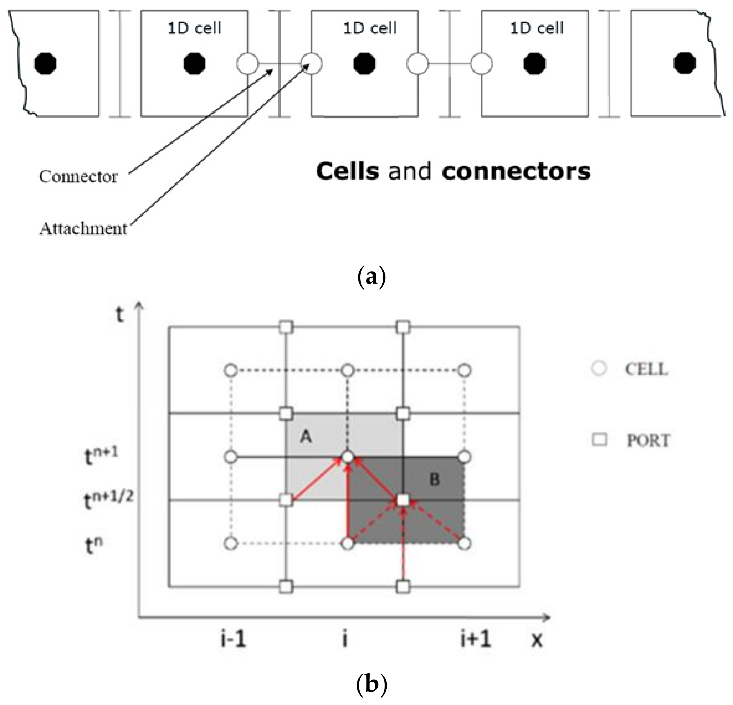Traditional numerical methods, based on finite difference techniques with 2nd order accuracy [11,12], behave as non-conservative when the calculation domain is so coarsely discretized [13]. Hence, an alternative numerical solver which ensures a good conservation with such large meshes has been applied, as briefly described below. The numerical method is a one-dimensional finite volume technique based on cells and connectors, named 1Dcell, explicit in time and 2nd order accurately derived from a quasi-3D formulation [14]. The transported quantities are defined in the cell centers, while their fluxes are established on the connectors. The space-time grid is staggered, as shown in Figure 1. The centers of the computational control volumes for the solution of the momentum equation are represented as small squares, while the cell control volume centers for the solution of mass and energy equations are represented by circles. They are located at different positions in both space and time.

With the above-mentioned reference frame, the continuity and energy conservation equations are solved with respect to the cell element, whereas the momentum equation is solved with respect to the connector elements between cells. The grid is also staggered in time as depicted by Figure 1. The closing equation is the perfect gas equation of state. The conservation equations of mass, energy and momentum are reported below:

$${\rho }_{cell}^{t+1}={\rho }_{cell}^t+\frac{∆t}{V}{\displaystyle \sum }_P^{Nports}{\left(\rho vA\right)}_P^{t+\frac{1}{2}}$$

(1)

$${\left(\rho e^0\right)}_{cell}^{t+1}={\left(\rho e^0\right)}_{cell}^t+\frac{∆t}{V}{\displaystyle \sum }_P^{Nports}{\left(\rho v{h}^{0}A\right)}_P^{t+\frac{1}{2}}+S_e$$

(2)

$${\left(\rho vA\right)}_{cell}^{t+\frac{1}{2}}={\left(\rho \overrightarrow{v}A\right)}_{cell}^{t-\frac{1}{2}}+\frac{∆t}{∆L}{\displaystyle \sum }_P^{Nports}\left[{\left(p+\rho v^2\right)}_P{A}_P\right]+S_M,$$

(3)

where $\rho$ is the gas density, $p$ is the gas pressure, $A$ is the pipe section and $V$ is the cell volume; $∆t$ and $∆x$ the time step size and the distance between cell centers, respectively; $h^0$ is the total enthalpy of the cell; $e^0$ is the total internal energy of the cell; $S_e$ and $S_m$ terms are the sources of the corresponding equations which consider heat transfer and friction with the duct wall.

This 1Dcell method has been applied for the solution with coarse meshes, to achieve a robust fast simulation method (FSM). Regarding the accurate solution in the case of ordinary mesh sizes (1 cm), the Corberán–Gascon TVD, finite difference, symmetric, explicit method was applied [15]. The TVD feature of this explicit method allows the reduction of the intrinsic instabilities or spurious oscillations which may appear using the explicit formulation. For both numerical methods, the time step is computed according to the Courant–Friedrichs–Lewy condition described by [16].

Intra-pipe boundary conditions are treated resorting to a characteristic-based approach [11,16] to handle junctions, valves, sudden area changes, intercoolers and turbochargers. In particular, for pressure loss junctions experimentally derived loss coefficients are used. These data are available from the literature and are obtained mainly in steady-state flow conditions. Similarly, for poppet valves, measured flow coefficients have been used. Their applicability can be argued but, in any case, they allow a good representation of the physical phenomena with a reasonable approximation. The coupling with 3D models can be realized, improving the accuracy of the simulation, but this brings, as expected, an increase of computational burden that cannot be accepted when the calculation of a driving cycle is addressed [9]. A major concern in this type of simulation is also the approximation introduced by the modeling of the turbocharger. Usually, the compressor and the turbine are treated relying on performance maps, obtained experimentally in state-state flow conditions. The maps are provided by the supplier of the turbocharger or, alternatively, they can be obtained by measuring the turbocharger performances on the test bench [17]. In both cases, the result is a discrete map where information is available for specific revolution speeds. To extend the validity of the maps in regions outside of the experimental ones and between the single iso-velocity lines, interpolation techniques are used. The reliability of the procedure depends mainly on the interpolation technique adopted, but also on the pre-processing of the raw data of the map, which needs to be properly smoothed [18]. Alternatively, a few 1D models can solve the 1D conservation equations for the stator and the rotor, considering the effect of the rotation of the turbine and compressor wheel [19,20]. These are known as map-less approaches, which have a reduced level of approximation, but they need in any case a bit of calibration and detailed data about the turbo geometry. This approach, going in the direction of a better approximation, brings the increase of the computational burden, which, once again, cannot be accepted when the goal is to reach a real-time simulation of a driving cycle.

3. Engine Description

The engine considered is a 6.7 L, turbocharged Diesel engine for heavy-duty applications such as buses and trucks, developed by FPT Industrial. This engine belongs to a commercial family, with a maximum power ranging from 184 kW to 235 kW. In this work, the medium-size 210 kW engine has been investigated.

Specific information about the engines studied is summarized in

Table 1. Engine geometrical data.

Quantity	Value	Unit of Measure
Bore × Stroke	104 × 132	mm × mm
Rod Length	195	mm
Number of Cylinders	6 (In-Line)	-
Total Displacement	6728	cm3
Compression Ratio	17	-
Valves per Cylinder	4	-

and

Table 2. Engine performance data.

Quantity	Value	Unit of Measure
Rotational Speed Range	600 ÷ 2600	rpm
Maximum Brake Torque	1010	Nm
Maximum Brake Power	210	kW

.

The engine is equipped with a twin-entry turbocharger characterized by a fixed geometry and a wastegate valve.

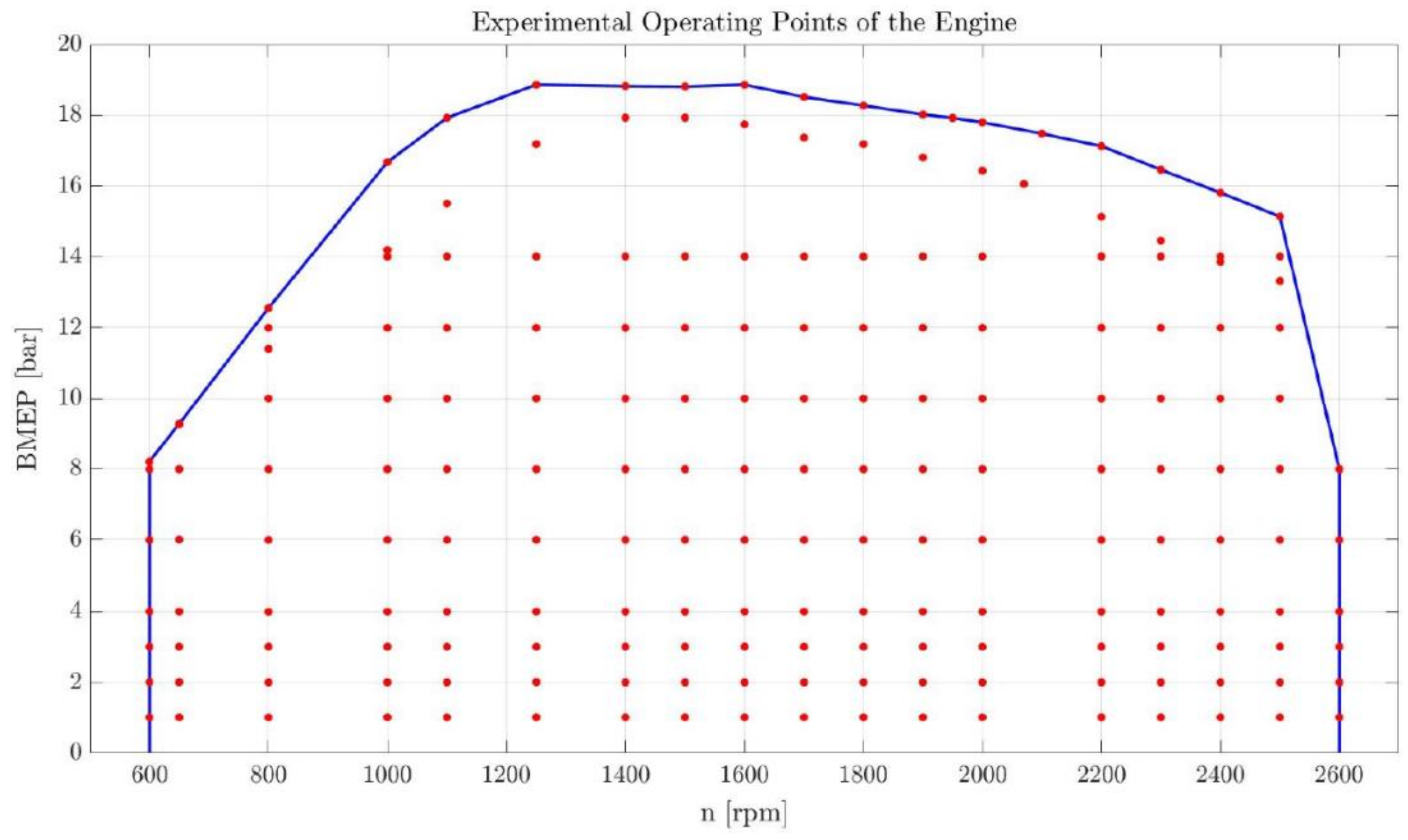
A wide set of experimental data was available to validate the engine thermo-fluid dynamic model. All these data refer to different steady-state operating points, defined by engine speed and brake mean effective pressure (BMEP). The operating map of the 210 kW engine, investigated in this study, is represented by the red points in Figure 2.

4. Calculation Methodology

As anticipated, the final aim of this work is to carry out the transient simulation of the IC engine integrated with a complete vehicle model, considering the real driving conditions. The analysis conducted is summarized by the following steps:

• development of the engine simulation model.
• validation of the model at fixed point operating conditions.
• vehicle and engine model integration.
• vehicle dynamics simulation in real driving conditions.

During the first two steps of the activity, the 1D engine model is refined and then validated under steady-state conditions throughout the whole engine map. The simulation code iterates the calculation by studying all the operating points in sequence. Once the results obtained match the experimental data with minor discrepancy, the simulation of transient operation of the engine can be investigated through step 3 and step 4. The 1D model is reported in Figure 3.

Relying on the coupling functionality of the simulation tool, the 1D engine model can be exported to the Simulink^® environment by means of an S-Function block. This possibility is exploited for the vehicle simulation, which is performed by means of the vehicle tool: this software is a Simulink^® add-on that allows the simulation of the longitudinal dynamics of vehicles with a large variety of architectures [21]. The vehicle model consists of different sub-system blocks, each one in charge of a specific task, to represent the specific devices along the powertrain such as gearbox, electric motor, and battery as described with more details in [4].

The IC engine model operating in transient conditions is represented by the simplified scheme reported in Figure 4.

In Figure 4 the S-Function block in light yellow contains the engine 0D/1D thermo-fluid dynamic model, which acts as virtual engine solver. All the parameters to be set or monitored and controlled while the engine is running are highlighted in the green and blue box.

The complete transient model receives as input the target torque and the engine speed as function of time: these are used to define the required engine parameters for the current engine speed and load by means of interpolation tables. The controllers (green blocks) determine the actuated quantities such as injected fuel mass, wastegate valve opening and inter-cooler wall temperature, which enter the virtual engine S-Function. Finally, the S-Function block provides the desired outputs.

This complete engine model, operating in transient conditions, can be coupled to the conventional vehicle model, improving the basic representation of the IC engine by means of measured steady-state operating maps. The standard vehicle simulation tool reproduces the behavior of the different vehicle components, including the engine, by pre-determined tables and via interpolation, every output quantity requested can be instantly calculated without considering the dynamics of the device.

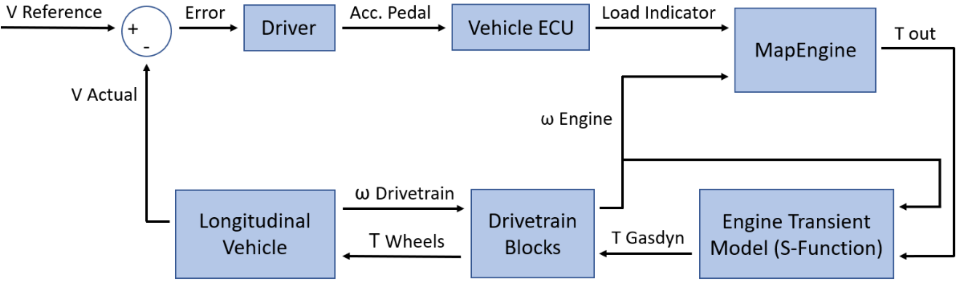
To introduce the engine model by an S-Function block, the pre-existent vehicle velocity control is modified as reported in Figure 5, which shows the simulation architecture.

While in the conventional approach, the output torque of the engine is simply determined via interpolation of the engine maps. The proposed methodology instead asks the running engine model to produce the required torque. This implies that the output torque of the engine might not be equal to the target but reflects the fluid dynamic solution obtained, hence it is affected by the intrinsic inertia and unsteadiness of the engine. It is the actual torque produced by the engine that is fed to the vehicle dynamics.

5. Calibration of Engine Model

An important step is related to the calibration of the 1D thermo-fluid dynamic model of the engine; in particular, the set up and consequent tuning of the combustion model is fundamental to achieve reliable results.

5.1. Description of Complete Engine Model

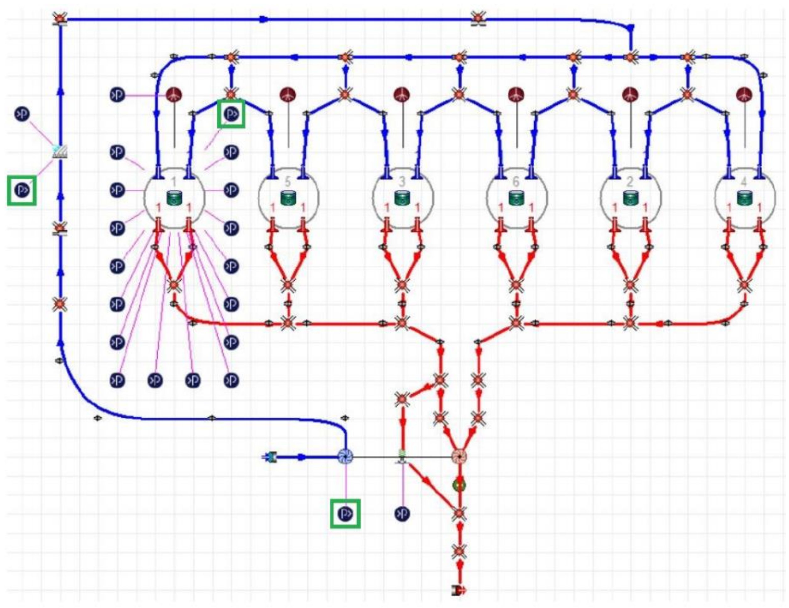
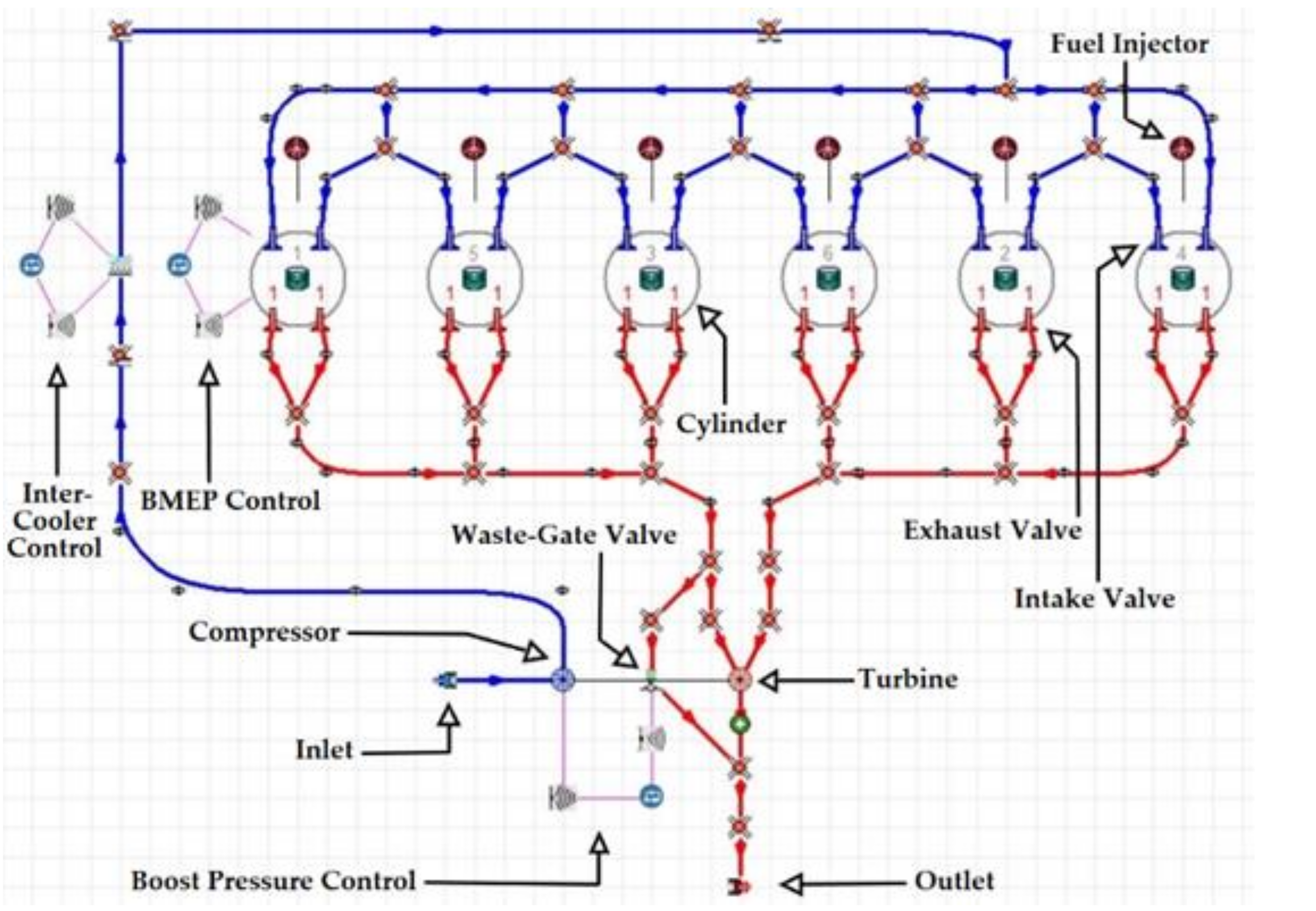
The 6-cylinder turbocharged Diesel engine schematic is reported in Figure 6, highlighting the typical components introduced for the simulation.

Figure 6 shows the air and exhaust gas paths, including the compressor and the fixed geometry twin-entry turbine with a waste-gate valve. Six fuel injectors are present, together with dedicated controllers for intercooler outlet temperature and engine BMEP, to make the engine work in the same operating points of the experimental campaign. In the case of steady-state operating points, the engine cycles calculations are performed until convergence to the targets is reached.

It is important to underline that the model does not feature any after-treatment system (ATS) and that the transport of chemical species along the ducts was not activated: this means that the emissions could be evaluated only as cylinder-out.

The calibration procedure of the model was carried out with a detailed 1D schematic, with a very refined mesh. After that, the subsequent simulations with the complete engine-vehicle system were based on the FSM approach with a coarse mesh, to achieve a significant reduction of the computational burden preserving the accuracy.

5.2. Engine Model Calibration

The CI engine combustion process is modeled with this approach: the cylinder volume is considered as a 0D system, in which the different chemical species are accounted for by a mixture of ideal gases. The process takes place with closed valves and is governed by the following energy equation (1st law of thermodynamics) [22]:

$$\frac{\mathrm{V}}{\overline{\mathsf{\gamma }}-1}·\frac{\mathrm{dP}}{\mathrm{d}\mathsf{\theta }}+\frac{\overline{\mathsf{\gamma }}}{\overline{\mathsf{\gamma }}-1}·\mathrm{P}·\frac{\mathrm{dV}}{\mathrm{d}\mathsf{\theta }}={\mathrm{m}}_{\mathrm{F}}·\mathrm{LHV}·\frac{{\mathrm{dx}}_{\mathrm{b}}}{\mathrm{d}\mathsf{\theta }}·{\mathsf{\eta }}_{\mathrm{c}}-\frac{{\dot{\mathrm{Q}}}_{\mathrm{w}}}{\mathsf{\omega }}$$

(4)

where V is the instantaneous in-cylinder volume, P the in-cylinder pressure (known from the experimental pressure traces), $\overline{\mathsf{\gamma }}$ the average adiabatic constant of the equivalent gas mixture, θ the crank angle, m_F the injected fuel mass (per cylinder per cycle), LHV the lower heating value of the fuel, x_b the “fuel burnt mass fraction” (i.e., the mass fraction of fuel that has already taken part to the combustion, at a specific crank angle position), η_c the efficiency of the combustion process, ${\dot{\mathrm{Q}}}_{\mathrm{w}}$ the heat loss through the cylinder walls and ω the crankshaft angular speed. In the energy balance, the unknown to be computed is x_b.

In Equation (4), the left side member is the so-called “actual heat release rate” (AHRR), an energy contribution due to pressure and volume variation representing the energy effectively used to produce work. This term equals the difference between the “heat release rate” (HRR) by fuel combustion and the heat losses through the cylinder walls.

While the quantities AHRR and HRR have a known expression, the heat losses typically do not. The simple application of predictive formulas such as the Woschni model [23,24] ([6,7]) does not guarantee a reliable calculation of this term, since those models need to be recalibrated for each test case (as documented in [25,26]). Hence, by integrating Equation (4) during the combustion phase, it is possible to write that:

$${\mathrm{Q}}_{\mathrm{w},\mathrm{tot}}={{\displaystyle \int }}_{{\mathsf{\theta }}_{\mathrm{i}}}^{{\mathsf{\theta }}_{\mathrm{f}}}\frac{{\dot{\mathrm{Q}}}_{\mathrm{w}}}{\mathsf{\omega }}\mathrm{d}\mathsf{\theta }={\mathrm{m}}_{\mathrm{F}}·\mathrm{LHV}-\underset{{\mathsf{\theta }}_{\mathrm{i}}}{\overset{{\mathsf{\theta }}_{\mathrm{f}}}{{\displaystyle \int }}}\left(\frac{\mathrm{V}}{\overline{\mathsf{\gamma }}-1}·\frac{\mathrm{dP}}{\mathrm{d}\mathsf{\theta }}+\frac{\overline{\mathsf{\gamma }}}{\overline{\mathsf{\gamma }}-1}·\mathrm{P}·\frac{\mathrm{dV}}{\mathrm{d}\mathsf{\theta }}\right)\mathrm{d}\mathsf{\theta }$$

(5)

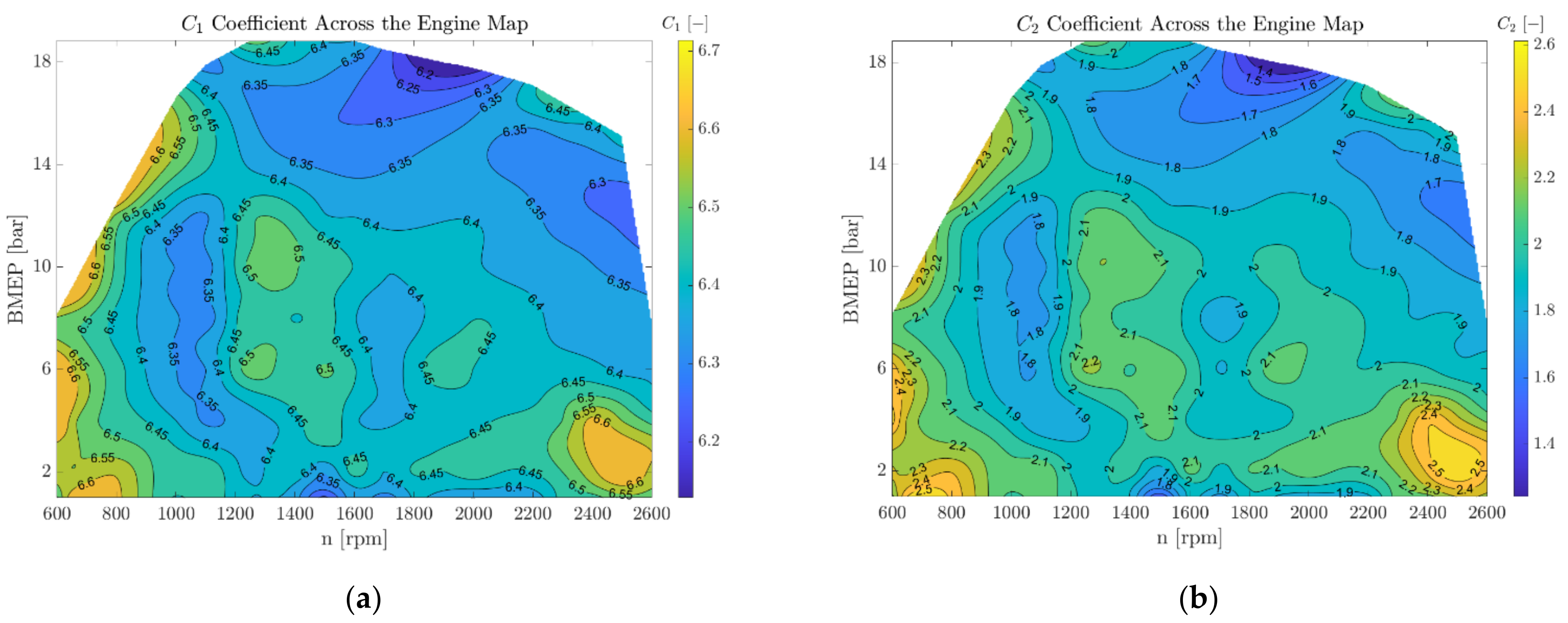
where ${\mathrm{Q}}_{\mathrm{w},\mathrm{tot}}$_t is the total heat exchanged during combustion, by assuming the combustion efficiency η_c equal to 1. This quantity can be computed for all the engine map operating points, once the in-cylinder pressure is known by measurements and used to calibrate the Woschni model point by point. In this work the tuning has been carried out by means of the two coefficients and (for more details please refer to [23,24]) and by minimizing the following error function for each operating point:

$$z\left(C_1,C_2\right)=\left|\frac{Q_{w,tot}-Q_w\left(C_1,C_2\right)}{\mathrm{CHR}}\right|$$

(6)

where CHR is the cumulative heat release, and $Q_w$ ($C_1$, $C_2$) is the computed wall heat exchanged for a given set of values ($C_1$, $C_2$). The distribution of $C_1$ and $C_2$ values on the engine map is shown in Figure 7. To retain a simpler set of $C_1$ and $C_2$ coefficients to be inserted in the 1D simulation model, their distribution on the engine map has been averaged along the BMEP axis, achieving a dependence only on engine speed.

A little distortion in the distribution can be seen in some full load points: hence, these values have been reconstructed based on the adjacent points.

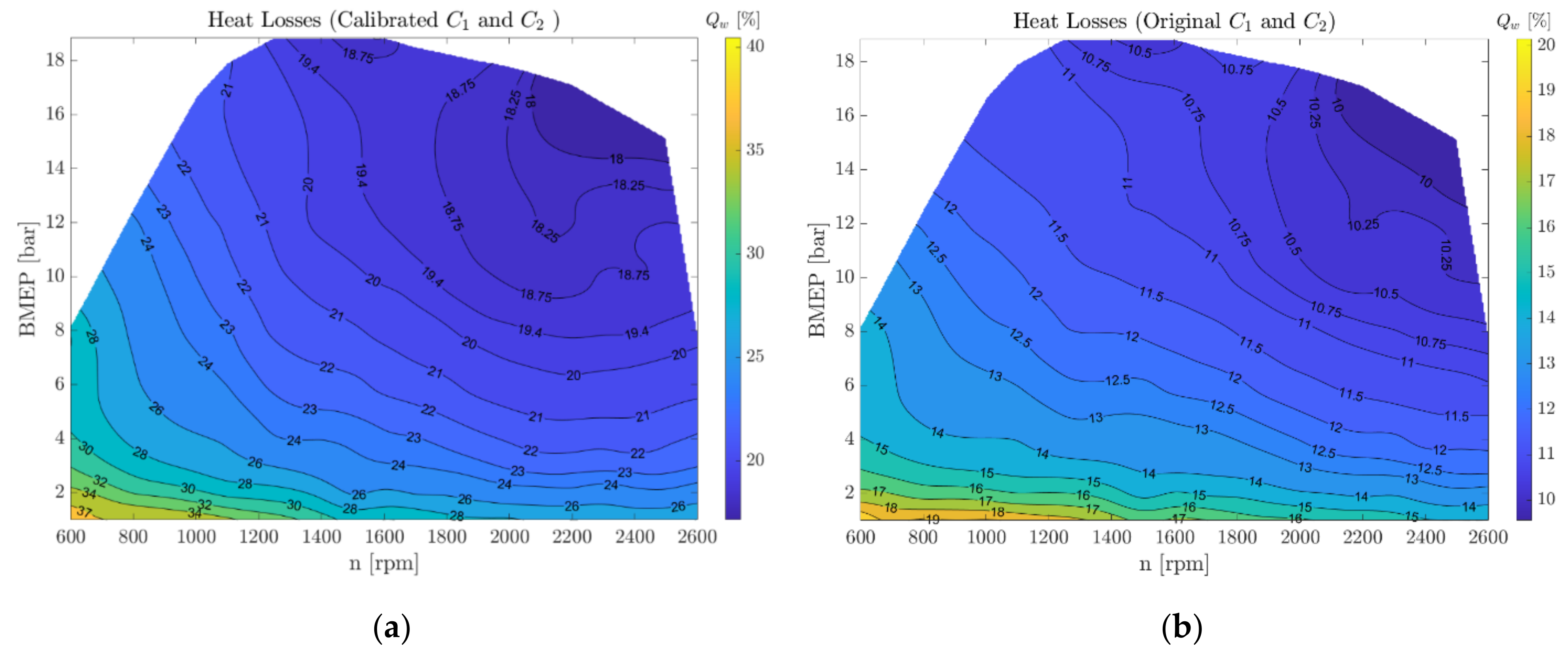
The total heat losses during the combustion process can be computed by applying the Woschni model, as reported in Figure 8, where the heat loss is expressed as a percentage of the total heat released by fuel combustion (i.e., simply, assuming η_c = 1).

As shown by the contour plots of Figure 8, the recalibration of Woschni’s formula is fundamental to correctly evaluate the heat loss term, especially for medium-large displacements such as the one considered: without this tuning process, the heat losses would have been underestimated almost by a factor of two.

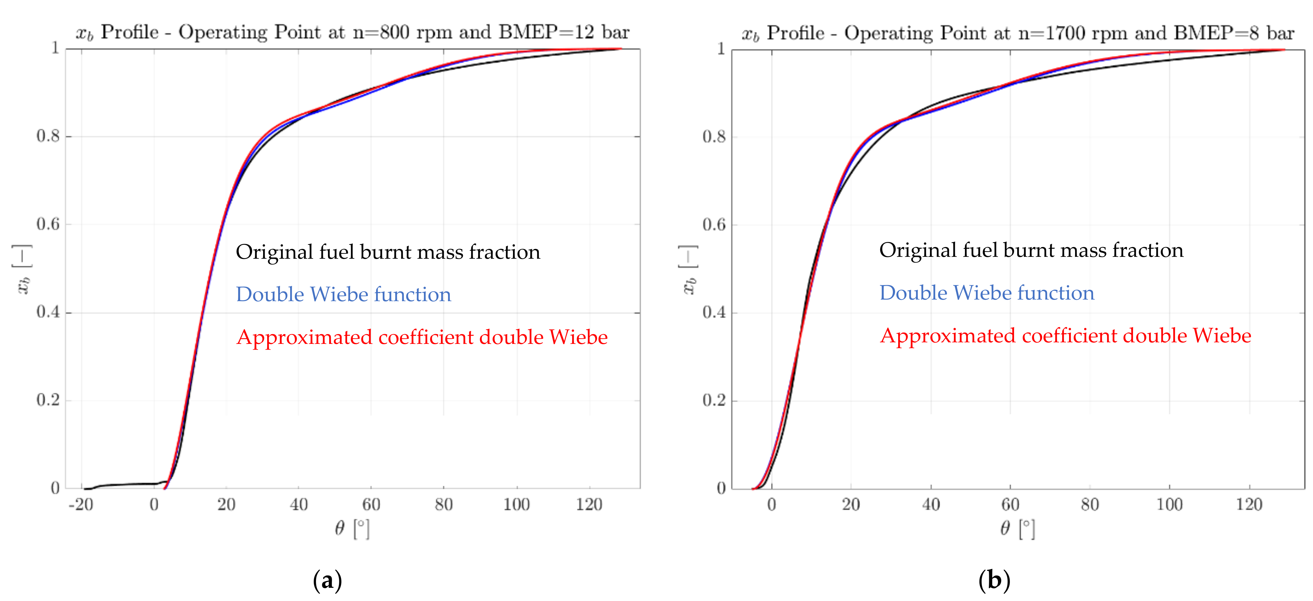
The fuel burnt mass fraction x_b can be computed once the energy balance has been verified. The calculation is performed by integrating Equation (5), which is implicit and non-linear, since $\overline{\mathsf{\gamma }}$ depends on the chemical composition, which varies during the combustion. Once the x_b profiles are computed for each sampled operating point, they must be extended across the entire engine map, since the engine could run in whichever working condition. Instead of interpolating among the calculated profiles, which are functions defined over different domains, it is advisable to approximate them by an analytical function (in this case the “double Wiebe’s” one) and then interpolate the fitting coefficients of these functions. The double Wiebe’s function can be written as follows (Equation (7)) [27]:

$${\mathrm{x}}_{\mathrm{b}}\left(\mathsf{\theta }\right)=\mathsf{\beta }·\left(1-{\mathrm{e}}^{-{\mathrm{a}}_1·{\left(\frac{\mathsf{\theta }-{\mathsf{\theta }}_{\mathrm{i},1}}{{\mathsf{\theta }}_{\mathrm{f},1}-{\mathsf{\theta }}_{\mathrm{i},1}}\right)}^{{\mathrm{m}}_1+1}}\right)+\left(1-\mathsf{\beta }\right)·\left(1-{\mathrm{e}}^{-{\mathrm{a}}_2·{\left(\frac{\mathsf{\theta }-{\mathsf{\theta }}_{\mathrm{i},2}}{{\mathsf{\theta }}_{\mathrm{f},2}-{\mathsf{\theta }}_{\mathrm{i},2}}\right)}^{{\mathrm{m}}_2+1}}\right)$$

(7)

where β is the “weight factor”, a₁ and a₂ are the “efficiency parameters”, m₁ and m₂ the “shape factors”, θ_i,1 and θ_i,2 the “starts of combustion”, θ_f,1 and θ_f,2 the “ends of combustion”. The fitting is performed by means of MATLAB^® built-in algorithms and the only parameters used are β, θ_f,1, m₁ and m₂; moreover, the following hypotheses are done:

• a₁ = a₂ = 6.9078 (complete combustion);
• θ_i,1 = θ_i,2 = SOC_main (the start of combustion is set with respect to the ignition of the main injection, since very little fuel is injected in the operating points with a pilot injection);
• θ_i,1 = θ_i,2 ≤ θ_f,1 ≤ θ_f,2 = EVO (exhaust valve opening);
• 0 ≤ β ≤ 1;
• 0 ≤ m₁, m₂ ≤ 1.

Once the fitting coefficients are defined for all the sampled points, their distribution across the engine map is further approximated with polynomial surfaces as function of engine speed and BMEP, to remove local distortions and have an easy computation of the coefficients for any combination of engine speeds and loads.

A comparison for the computed trends of the fuel burnt mass fraction x_b is represented in Figure 9, for two operating points as examples.

The profiles calculated by polynomial approximation are then considered for the remaining part of this study, given the satisfactory approximation they can provide.

6. Steady-State Map Results

After simulating all the map operating points, the predicted results can be collected and represented by means of contour plots, indexed by engine speed and load, which are used to identify the engine working conditions. These contour plots can be addressed as the steady-state maps of the IC engine, each one detailing a particular property. This kind of representation offers a quick, graphical way to verify the satisfactory correspondence between simulation results and experimental data.

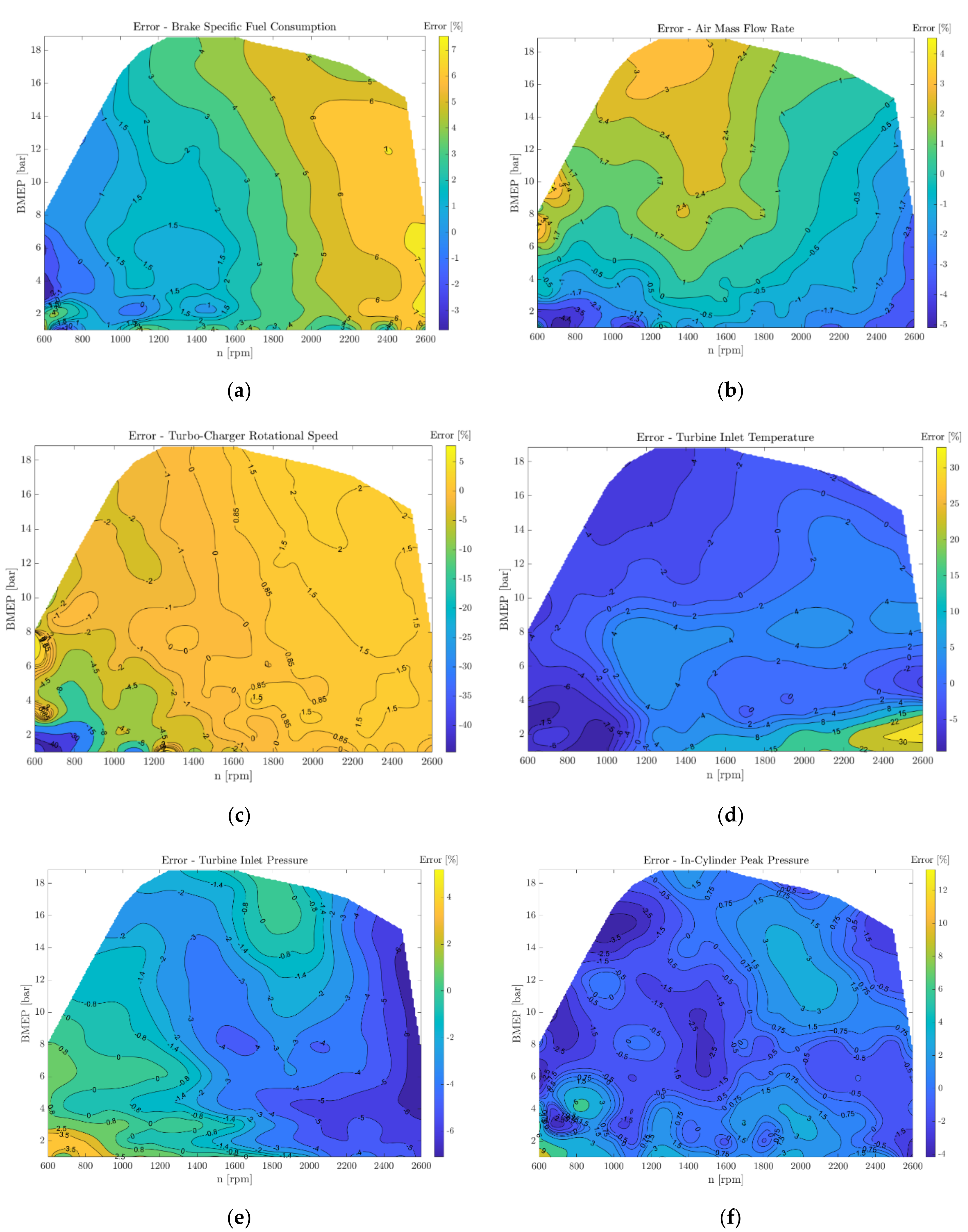
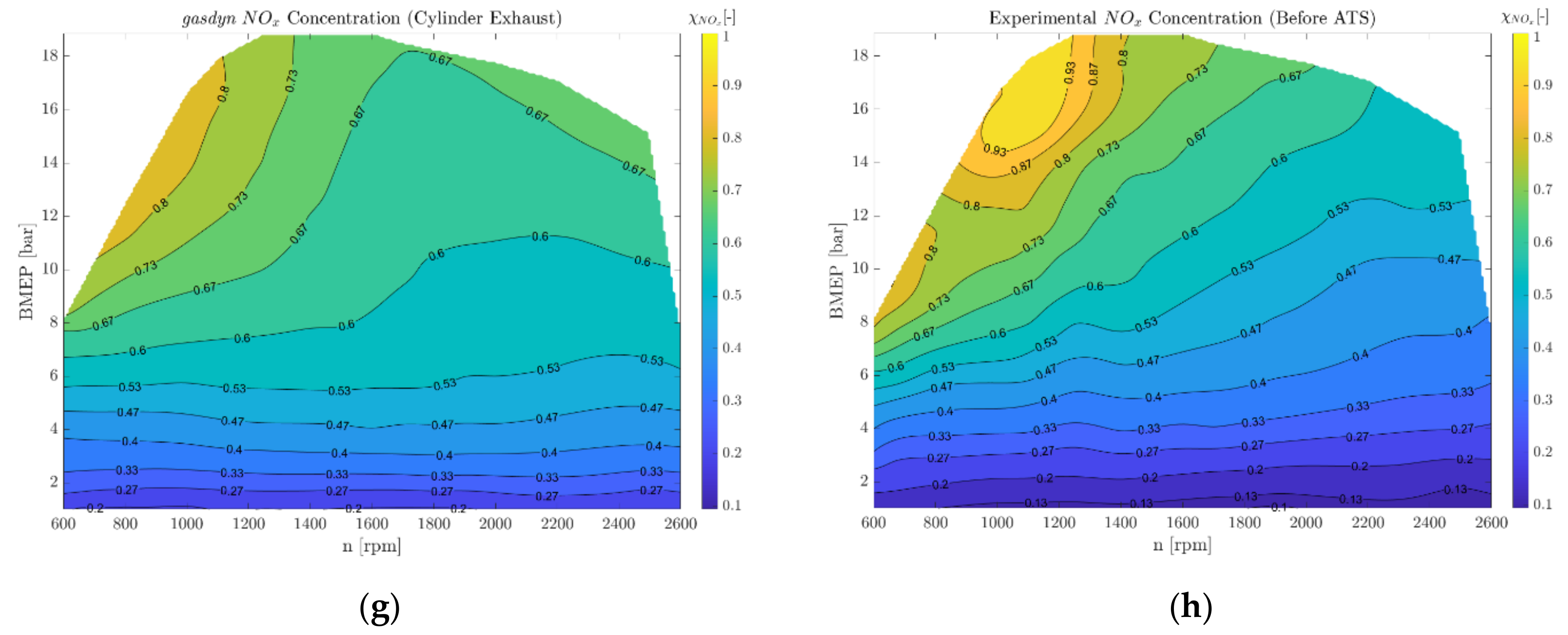
As an example, Figure 10 shows a group of steady-state maps referring to the most important engine performance and emission characteristics: in particular, Figure 10a–f highlight the discrepancy between measured and calculated results in terms of percentage error, whereas Figure 10g,h directly show the measured and simulated (non-dimensional) cylinder-out NOx emissions.

The prediction of specific fuel consumption by means of the 0D/1D code is very accurate at low and medium engine speeds, as reported in Figure 10a, whereas a larger discrepancy can be found at high regimes. However, considering the typical applications of the engine investigated, that part of the engine map is not frequently exploited, so that a reliable evaluation of fuel consumption is expected during an RDE test cycle.

Considering further important engine parameters (Figure 10b–f), the percentage errors are very small and local distortions can be acceptable at the edge of the maps (typically due to interpolation issues). Finally, the calculated NOx emission map (Figure 10g) agrees with the corresponding measured trends and values (Figure 10h), represented in normalized form with respect to the maximum experimental value. The satisfactory comparison confirms the good set-up of the combustion model, being NOx formation dependent on the correct prediction of in-cylinder temperature and local air-to-fuel ratio. The most important result of this activity is that the engine model can be run across non-mapped conditions reflecting the behavior of the real engine. When the model runs in transient, interpolations are performed to set up the engine model exploiting the know values of the nearest mapped operating conditions parameters.

7. Description of Vehicle and Test Cycles

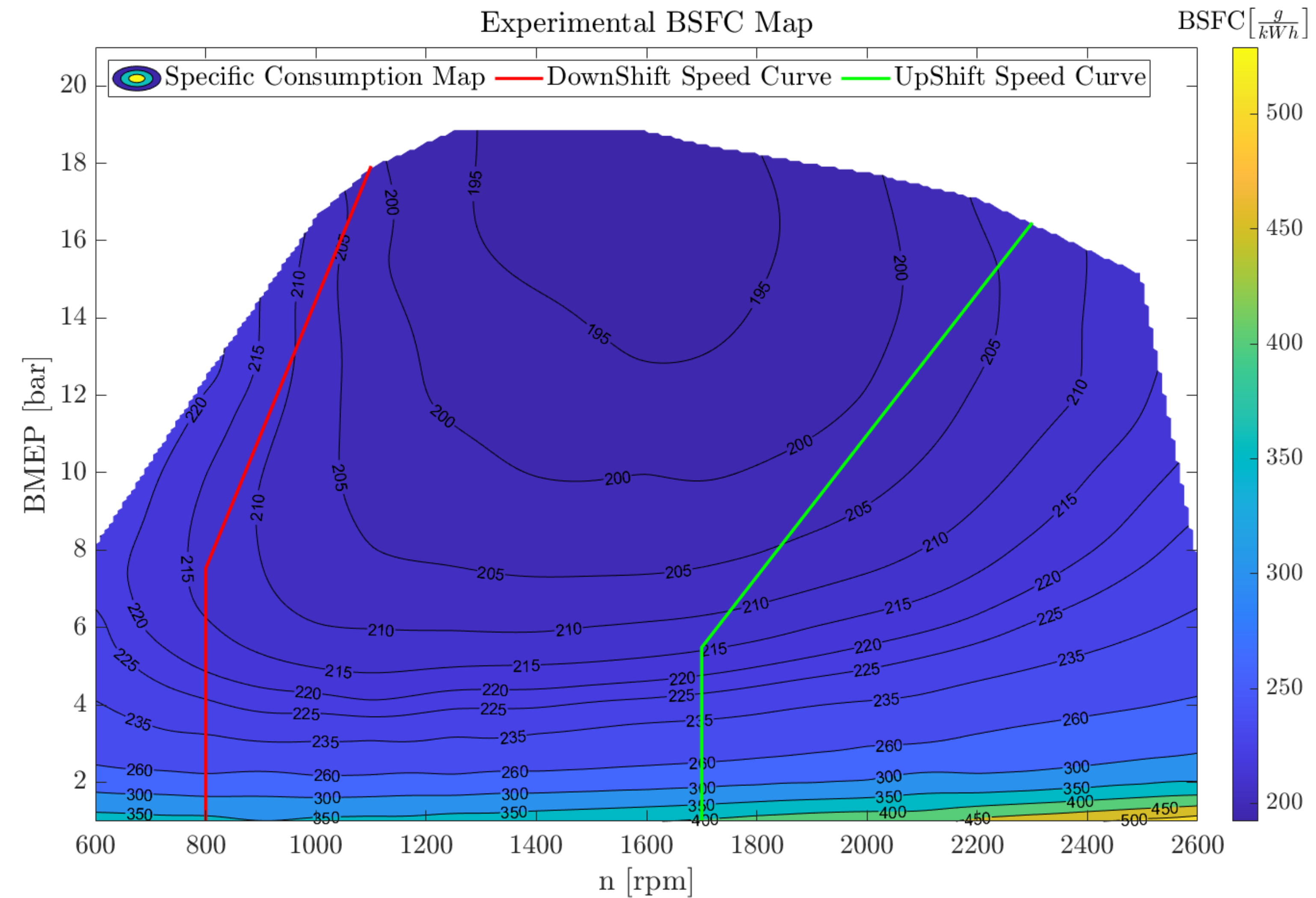
The vehicle used for the simulations is an interurban hybrid bus, which is coupled to the six-cylinder Diesel engine analyzed for this investigation. The main characteristics of this vehicle (mass, size, gearbox ratios, target mission) with a classical architecture were taken from the literature. Moreover, it is assumed that the vehicle runs on medium payload, with an overall vehicle mass equal to 12,600 kg. In the simulations, the vehicle is equipped with a six-speed manual gearbox and, according to the software gear shifting strategy, the gear shift lines are placed to allow the engine to work in its high efficiency region and to prevent it from running at excessive speeds. These lines are represented by engine torque and speed curves in Figure 11.

To calculate the vehicle longitudinal dynamics, all the vehicle model blocks are provided with the requested architecture-layout data. Firstly, the simulations are carried out on the Diesel bus version with manual transmission. Then, a full hybrid parallel P2 configuration of the bus has been set up and investigated. The electric motor, placed between the engine flywheel and the gear box is a permanent magnet synchronous one. A “torque split” algorithm, together with a first-order thermal model, is used to test and validate the motor, which is simulated through steady-state maps. To match the different engine and motor speed ranges, a reduction gear connects the latter to the drive shaft between the clutches. The system is powered by a lithium-ion battery pack, characterized by a 1p110s (1 parallel, 110 series) arrangement working at 400 V, which has been designed taking into account the peak-power request, calculated by means of the “torque split” algorithm adopted, and of the overall energy storage requirements.

Once the electric components are chosen, a proper tuning of the hybrid control unit (HCU) is performed in the vehicle simulation tool, acting on the specific torque-speed curves that define the operating mode of the hybrid system, and the battery SoC (state of charge) threshold levels [28]. As mentioned, a first set of parameters to be defined is represented by the torque curves, which are indexed by the revolution speed, generalized to the drive shaft between the clutches. These curves characterize different regions on a torque-speed plane: depending on the total torque required by the vehicle and its actual speed, the position of such working condition on the torque-speed plane determines the hybrid system operating mode. For the hybrid architecture considered, the torque-speed curves are referred to the engine BSFC map: this allows their correct positioning, aimed at reaching the best overall efficiency.

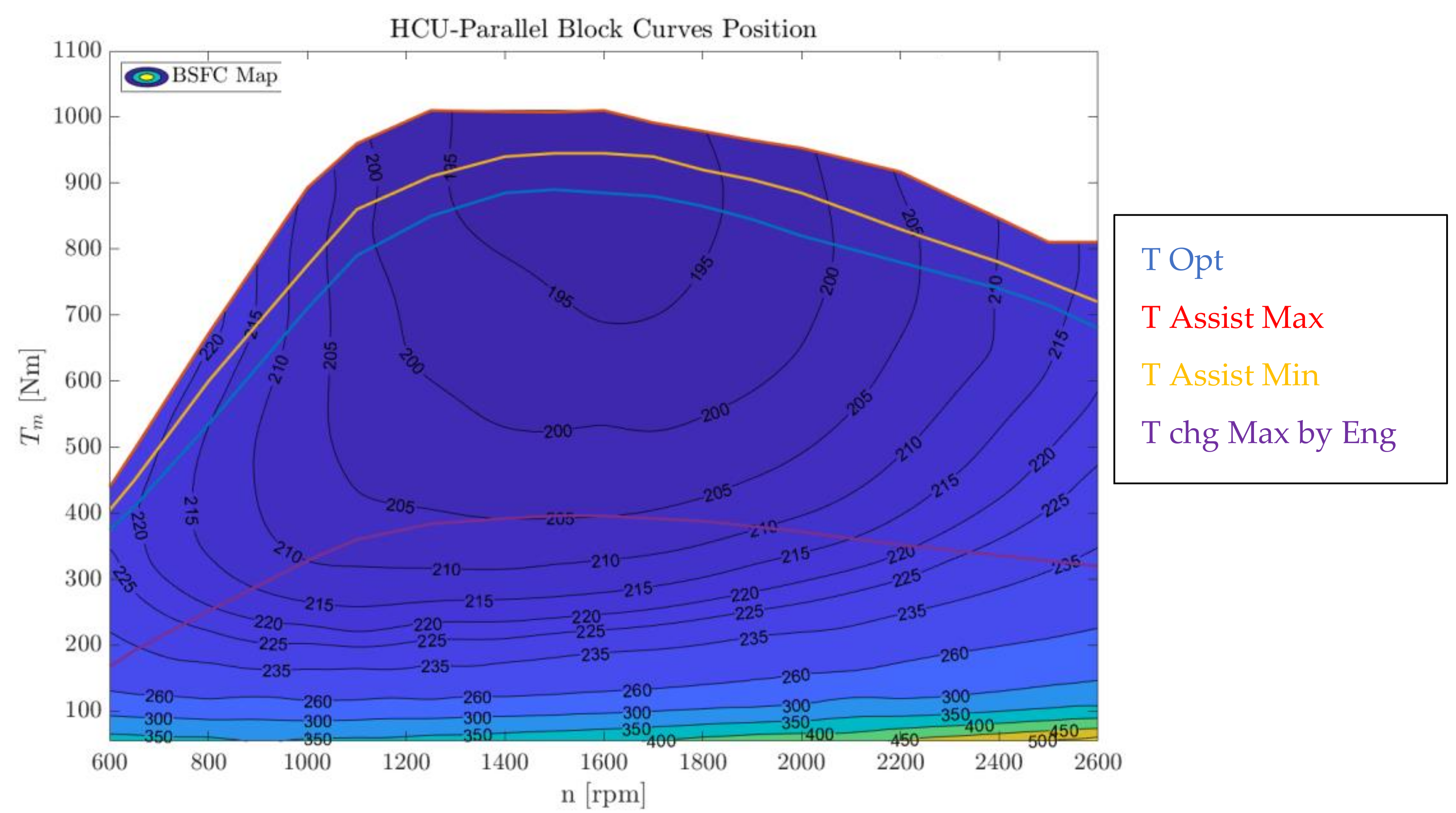
In Figure 12, it is possible to distinguish four different curves, cited with their actual name in the vehicle simulation tool. To correctly place these curves, the underlying rationale of the hybrid powertrain must be pursued: letting the engine work in its high-efficiency regions.

The lowest purple line defines a map region below which the engine is generally prevented from working: when the requested engine torque lies below this curve, the HCU determines an increase of torque request, so as to bring the operating point above the purple line. Then, the torque surplus is used to charge the battery through the motor generator mode. This curve has been placed to achieve a compromise: it prevents the engine from working in low-efficiency points, such as the bottom part of the map, so that above this curve an optimal operation of the engine is achieved.

The region between the purple line and the yellow one defines the area in which the engine can work. If the required torque is located between the yellow line and the red one the engine is supported by the electric motor to provide the requested torque. The blue curve represents the maximum efficiency curve for the engine, to achieve the minimum fuel consumption and CO₂ production. It is important to remark that, due to the characteristics of this engine, the maximum efficiency is often located around the full load in the engine map. If the overall requested torque exceeds the full load torque of the engine, the additional torque requested is provided by the electric motor. The vehicle control unit also decides when to turn off and on the engine. It is important to highlight that the engine model has the capability to be turned off and on, with the corresponding effects on the fluid dynamic solution.

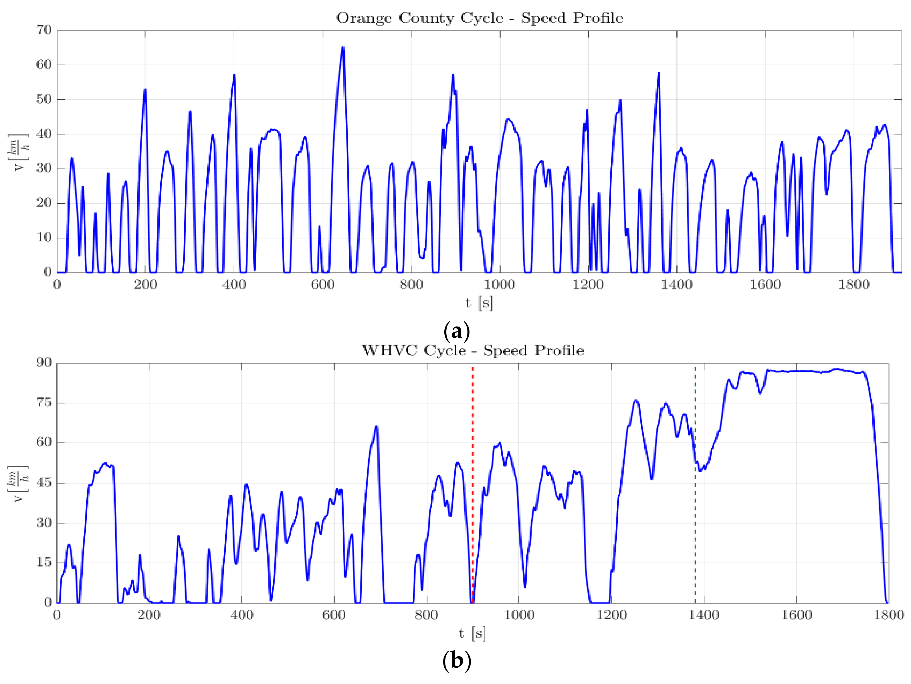
To evaluate the bus performance under various scenarios, two different missions were chosen. The first is the orange county (OC) cycle, a chassis test for heavy-duty vehicles such as buses. Its speed profile is depicted in Figure 13a: with relatively low speeds, but frequent and steep accelerations and decelerations. This cycle is suitable to test the bus in urban driving conditions. The second one is the world harmonized vehicle cycle (WHVC), a generic test for heavy-duty vehicles, usually used for research purposes to compare the vehicle and engine emissions, derived from its corresponding engine dynamometer cycle: the WHTC. By looking at Figure 13b, this driving cycle consists of three different phases: an urban one, from the start of the cycle until the red dotted line; a rural phase, limited by the red and green dashed lines; a motorway phase, in the last part of the cycle. The composition of the cycle makes it suitable to test the bus in various conditions, including travelling on extra-urban roads, during the rural and motorway phases. Further information about these cycles can be found in [29,30].

8. Vehicle Dynamics Simulations

The application and validation of this new co-simulation procedure are based on a direct comparison between two different approaches. In this section, for both bus versions (conventional Diesel and hybrid), the main outcomes of the map-based approach and the transient coupled model are reported and discussed. Only the results related to the WHVC cycle are shown since it represents a mixed mission able to test the new methodology into a wide range of accelerations and speeds, even if the full exploitation of a hybrid system can be reached in urban driving.

The fuel economy series for the different Diesel simulation models are collected in

Table 3. WHVC: Diesel bus fuel economy comparison.

Diesel Bus—Fuel Economy	$\mathbf{Value}\left[\frac{\mathbf{l}}{100\mathbf{km}}\right]$	Error [%]
Map-Based, Experimental 1	24.88	Reference
Map-Based, calculated points 2	25.57	2.77
Transient 3	25.8	3.7

¹ Map-Based approach with fuel consumption map from experimental data. ² Map-Based approach with fuel consumption map from engine model steady-state analysis. ³ Vehicle-engine transient model.

. The increase of fuel consumption for the transient model is probably due to the dynamics of the engine (inertia is considered with respect to the map-based steady-state model) as well as to a little overestimation of fuel consumption, as shown by Figure 10a and by the midway model (based on the map of fuel consumption, obtained by the analysis of steady-state operating conditions).

To carry out a fair comparison between the fuel consumption of the Diesel and hybrid versions, a normalization technique must be applied. The procedure devised by the “low carbon vehicle partnership” (LowCVP) and adopted in the United Kingdom is described in detail in [29]: intended just for buses, it perfectly fits the case considered in this work. According to this procedure, it is necessary to calculate a quantity called “net energy change” (NEC), expressed by the following formula:

NEC = (SoC_f − SoC_i)∙V_sys∙K₁

(8)

where SoC_f and SoC_i are respectively the final and initial battery state of charge expressed in [Ah] (calculated multiplying the battery capacity by the percentage state of charge), V_sys is the nominal DC operating voltage of the battery, and K₁ is a constant equal to 3600 s/h, necessary to pass from hours to seconds. Besides the NEC, two further quantities must be calculated. These are the “total fuel energy” (TFE) and the “total cycle energy” (TCE):

TFE = m_F,tot ∙ LHV

(9)

TCE = TFE − NEC

(10)

where m_F,tot is the total fuel mass consumed. The last formula (10) computes the total energy used to complete the driving cycle, provided by the fuel combustion and the battery. The final step is to calculate the “NEC variance” according to Equation (11) and check which range of

Table 4. Possible |NEC Variance| ranges.

|NEC Variance|	Description
≤1%	The fuel consumption measured in the cycle can be considered correct.
>1% ∧ ≤5%	The fuel consumption measured in the cycle needs to be corrected.
>5%	The vehicle run under analysis is not considered valid.

it falls into.

$$\left|\mathrm{NEC}\mathrm{Variance}\right|=\left|\frac{\mathrm{NEC}}{\mathrm{TCE}}·100\right|$$

(11)

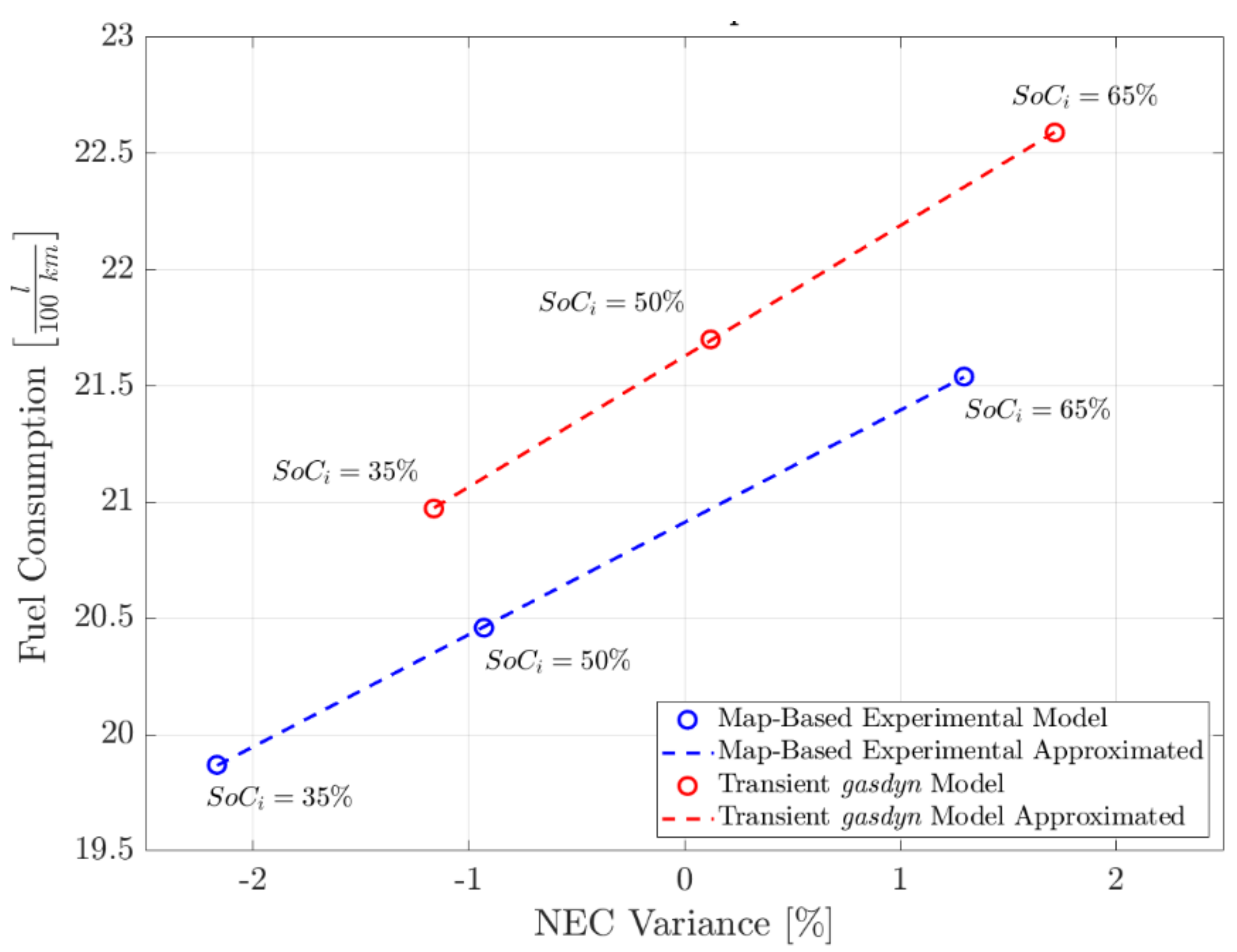
The correction requires to simulate the driving cycle multiple times, until getting three valid runs at least (i.e., each one with a |NEC Variance| ≤ 5%). Once this is achieved, each test run must be identified by an NEC Variance value and a fuel consumption; these points are then represented in a plane and processed with a linear regression (see Figure 14). If the “coefficient of linear correlation” of the regression is R² ≥ 0.8, then the set of points constitutes a family of valid test runs and the corrected fuel consumption is given by the linear regression straight line, evaluated at NEC Variance = 0%. Hence, as indicated by the normalization procedure, three different SoC_i are chosen: 35%, 50% and 65% for both the map-based experimental procedure and the transient simulation. Note that all six runs are valid (i.e., |NEC Variance| ≤ 5%).

The normalized fuel consumption, calculated for the hybrid vehicle by both simulation approaches, is collected in

Table 5. WHVC: Fuel economy for Diesel and hybrid bus architectures.

Bus Version and Simulation Approach	$$\begin{gathered} \mathbf{Fuel}\mathbf{Economy}\left[\frac{\mathbf{l}}{100\mathbf{km}}\right] \\ \left(\mathbf{Normalized}\mathbf{One}\mathbf{in}\mathbf{Case}\mathbf{of}\mathbf{the}\mathbf{Hybrid}\mathbf{Bus}\right) \end{gathered}$$
Map-Based Experimental 1 Diesel	24.88
Map-Based Experimental 1 hybrid	20.91
Transient 2 Diesel	25.8
Transient 2 hybrid	21.63

¹ Map-Based approach with fuel consumption from experimental data. ² Vehicle with engine transient model.

and directly compared to that for the conventional Diesel vehicle. As already discussed, the transient simulation model reveals slightly higher fuel consumption.

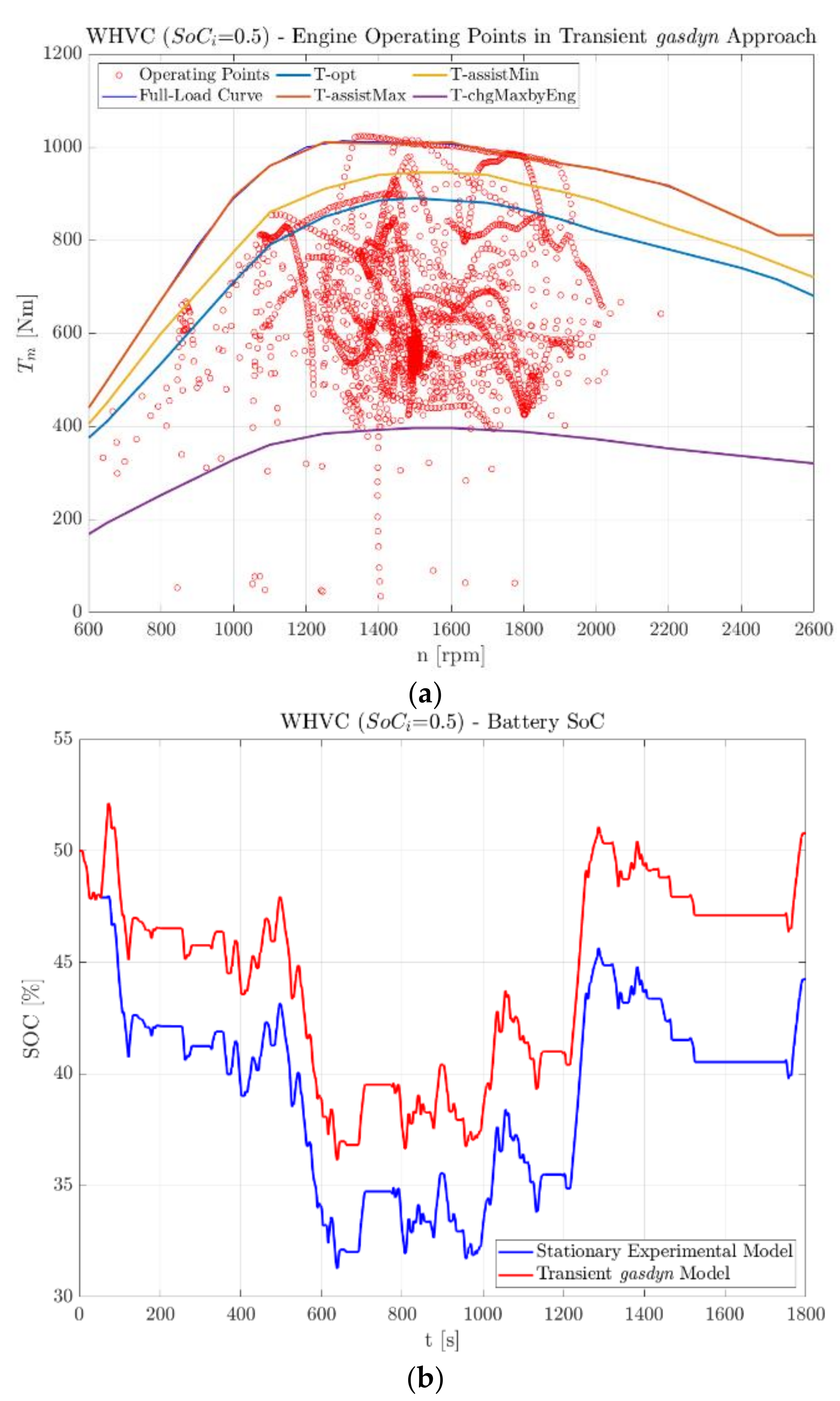
In Figure 15a, the resulting cloud of engine operating points during the WHVC test cycle with a SoC_i of 50%, simulated by the transient approach, are shown together with the HCU curves of Figure 12. The engine operation follows the rules of the logic previously described: it works very rarely where the engine is not efficient, except when the engine is off or it is turned on trying to the target operating condition. Figure 15b shows the SoC of the battery during the same run, calculated by both simulation methods. The two curves are similar, but not identical: this depends on how the HCU manages and uses the two sources of torque (i.e., the e-motor and the IC engine). It bases the splitting on the required torque at that time instant: since the requested torque can be a little bit different between the two modeling approaches (due to the influence of engine dynamics), a particular engine condition can fall into different HCU regions on the map. Therefore, the managing of the required torque can be different, as well as the SoC profile.

Moreover, the SoC at the end of simulation (SoC_i) reaches half of the battery storage energy. This convergence condition can be noticed for both the driving cycles and the three SoC_i values chosen, emphasizing the good design of the HCU logic.

Even if the WHVC is a mixed driving cycle, significant fuel savings can be achieved, probably mostly during its first phase: the urban drive. In fact, by comparing the Diesel and hybrid map-based calculations, the fuel economy improves by 15.96%, while for the hybrid transient simulation approach the reduction of fuel economy is equal to 16.16% (with respect to the Diesel transient model). Overall, a satisfactory agreement can be found, when comparing the two different powertrain architectures with the same modeling approach: independently of how the engine operation is calculated (through the map-based or transient method), the HCU is able to manage both, highlighting the advantages of the bus powertrain investigated in this work: the hybrid architecture.

Dealing with the simulation of RDE and WHTC test cycles, it is important to discuss the computational effort requested and the prediction accuracy achieved by the FSM (fast simulation method) methodology, compared to the standard solver applied to a 1D schematic with a refined mesh. This can be analyzed in terms of CPU time and of variation of engine output quantities. To this purpose, the simulation of the same WHTC cycle has been performed with both a refined mesh (1 cm) and a coarse one (10 cm with the FSM methodology). As shown in Figure 16a,b the reduction of computational effort is relevant, around 80% with respect to the same simulation in the refined mesh solution. To estimate if the accuracy has changed between the two approached, the cumulative fuel consumption and cylinder out emission are compared. As it can be seen, the two approaches differ by less than 1%, revealing that the overall accuracy has been preserved and that long-lasting driving cycle can be simulated by resorting to fast simulation strategies without introducing excessive approximations.

9. Conclusions

This research work focused on the prediction of fuel consumption of a Diesel heavy-duty engine in real driving cycles, by means of computer simulations. As investigated in previous works, the map-based approach (relying on tables derived through the engine steady-state analysis), to represent the IC engine characteristics within a vehicle model, can be very fast but it could also provide poor results in terms of fuel consumption and pollutants emissions, especially with new and demanding test cycles. In fact, this approach completely disregards the engine dynamics, which runs considering a simple sequence of steady-state points, with a sort of instantaneous transition from one to another.

To define a reliable simulation tool for the analysis of IC engines during transients, this work investigated the suitable coupling of a complete vehicle model to an IC engine model, interacting in real-time during an RDE.

A 0D/1D six-cylinder Diesel engine model has been developed and, with some calibration of its combustion model on the basis of the available experimental data, validated in steady-state (engine map) conditions. Hence, the study focused on the transient operation of the IC engine, which has been integrated into a complete vehicle model, by means of the Simulink^® environment and coupled to vehicle models. A conventional vehicle architecture has been compared to a hybrid architecture, to highlight the performances of the two solutions and the prediction of fuel consumption by means of the usual map-based approach and the transient approach.

Future developments could focus on the prediction of pollutant emissions under transient operation. In fact, the complete transient model built could provide the input data, in terms of cylinder-out emissions, to the after-treatment simulation model coupled to the IC engine itself, which could highlight the tailpipe emissions during different RDE cycles and strategies.