Numerical Validation of the Radiative Model for the Solar Cadaster Developed for Greater Geneva

Abstract

The achievement of the targets for reducing greenhouse gas emissions set by the Paris Agreements and the Swiss federal law on the reduction of greenhouse gas emissions (CO₂ law) requires massive use of renewable energies, which cannot be achieved without their adoption by the general public. The solar cadaster developed as part of the INTERREG G2 Solar project is intended to assess the solar potential of buildings at the scale of Greater Geneva—for both industrial buildings and for individual residential buildings—at a resolution of 1 m. The new version of the solar cadaster is intended to assess the solar potential of roofs, as well as that of vertical facades. The study presented here aims to validate this new version through a comparison with results obtained with two other simulation tools that are widely used and validated by the scientific community. The good accordance with the results obtained with ENVI-met and DIVA-for-Rhino demonstrates the capability of the radiative model developed for the solar cadaster of Greater Geneva to accurately predict the radiation levels of building facades in configurations with randomly distributed buildings (horizontally or vertically).

1. Introduction

The massive use of renewable energies and, more particularly, solar energy is necessary in order to meet the objectives of the Paris Agreements and the Swiss federal law on the reduction of greenhouse gas emissions (CO₂ law) [1]. As buildings are some of the main contributors to climate change, one of the main challenges is, therefore, turning buildings from energy consumers into energy producers. This cannot be done without the development of tools dedicated to the evaluation of solar potential.

This massive deployment involves the evaluation of solar potential on a large scale. In addition, the urban environment has many specific features that are to be taken into consideration when evaluating this potential. This can be achieved with solar cadasters.

However, these tools are usually limited to the evaluation of the solar potential on rooftops [2,3,4,5]. This limitation can be an obstacle to the development of the use of solar energy because the potential of vertical surfaces in an urban environment can prove to be predominant [6,7,8,9].

Thus, there is a need for large-scale tools that are able to take vertical facades into account, in addition to roofs. From a physical point of view, the effects of surrounding surfaces (the ground or surrounding buildings) on the vertical radiative balance are not well known and may appear to be non-negligible. From the point of view of solar production potential, the issues of the variability linked to shading effects are added. Tools that are able to consider these issues are being developed and need validation.

A solar cadaster tool is being developed at the scale of Greater Geneva, which is a trans-border agglomeration around the city of Geneva between France and Switzerland, and it totals an area of 2000 km². A first solar cadaster was developed for the Canton of Geneva only (280 km²), as presented by Desthieux et al. [10]. The goal now is to update and extend this solar cadaster for the whole of the Greater Geneva area in the framework of INTERREG G2 Solar. Its aim is to intensify solar energy production in the agglomeration by mobilizing a large panel of stakeholders from public institutions, municipalities, energy providers, the private sector, and universities. The difficulty lies in the fact that the solar cadaster must cover a large area (2000 km² for Greater Geneva) while providing accurate information at a small spatial resolution and with a reasonable computation time.

The main objective of this study is to validate a solar cadaster tool by using a comparison with the results from other numerical tools. To this purpose, the results from the solar cadaster are compared with those of two widely used tools: DIVA-for-Rhino and ENVI-met. The latter, thanks to its holistic model, makes it possible to deepen the assessment of the buildings’ photovoltaic potential by evaluating their surface temperatures.

The validation of the solar cadaster involves three different tools based on different models and methods and with a varied field of applications. Thus, these tools are presented first, prior to introducing the methodology used. The results in terms of predicted shortwave irradiance on both the roofs and the facades are then detailed and discussed.

2. Materials and Methods

2.1. Modeling Approaches for Radiative Transfers

Two main methods are commonly used for the evaluation of radiative transfers: ray-tracing-based models or radiosity methods. Their principles, as well as their advantages and drawbacks, are described in the following.

2.1.1. Ray-Tracing Methods

Ray-tracing methods consist of following the paths taken by electromagnetic rays. There are two types of ray-tracing approaches. Forward ray-tracing methods, also called light tracing, consist of launching rays from light sources in a set of directions. Backward ray-tracing methods consist of following the light path backward. In this latter case, rays are launched in a set of directions from the element of interest (the eye of an observer or an irradiated surface). A comparison between forward and backward ray tracing is illustrated in Figure 1.

For both of these methods, the directions can be random (probabilistic approach) or set (deterministic approach). After rays have been launched, an intersection test is carried out between each of these rays and the objects in the scene; then, new rays are cast from the points of impact while considering the properties of the materials encountered (reflection, transmission, absorption). This method makes it possible to take the effects of light into account, such as refraction of light (for example, in the case of a scene comprising glasses). The behavior of a ray at the point of intersection then depends on the refractive properties of the material encountered. This feature is particularly useful in the context of image synthesis or the study of transparent media with different refractive indexes.

This method also has the advantage of making the calculation of specular reflections possible (see Figure 2). On the other hand, it is not suitable for a calculation of diffuse reflections (which are usually the case for urban surfaces), as these require a significant calculation time because of the number of rays to be launched (in all directions) at each new intersection. This method has to be coupled with a diffuse radiation model.

2.1.2. Radiosity Method

The radiosity method is based on the calculation of the balance of radiosity, which is the total radiative flux exiting a surface ($\mathrm{W} {\mathrm{m}}^{-2}$). This method allows the calculation of diffuse and reflected components of the irradiation only by solving a system of equations involving all the objects of a scene. Taking specular reflections (see Figure 2) into account is not directly possible with this method. However, unlike ray tracing, the calculations are independent of the position of the possible observer (surface of interest)—the calculation is generalized over the whole scene.

The radiosity method is based on solving the equation introduced by Kajiya [11] and detailed in the work of Sillion and Puech [12], where the exiting power is expressed as:

$$B\left(x\right)=E\left(x\right)+\rho {\int }_{\mathsf{\Omega }}{L}_i\left(x,\theta ,\varphi \right)cos\theta \mathrm{d}\omega$$

(1)

where x is a point in space, $B\left(x\right)$ is the exiting power (emitted, reflected, and transmitted) at point x in space (in $\mathrm{W} {\mathrm{m}}^{-2}$), $E\left(x\right)$ is the power emitted by point x (source term, in $\mathrm{W} {\mathrm{m}}^{-2}$), $\rho$ is the coefficient of reflection of the surface, $L_i\left(x,\theta ,\varphi \right)$ is the incident power at point x from the solid angle determined by the angles $\theta$ and $\varphi$, $\mathsf{\Omega }$ is the set of directions $\left(\theta ,\varphi \right)$ of the hemisphere, and $\mathrm{d}\omega$ is the elementary solid angle ($\mathrm{sr}$).

This equation can be discretized:

$$B_i=E_i+{\rho }_i\sum _{j=1}^N{F}_{ij}{B}_j$$

(2)

where $B_i$ and $B_j$ are the power exiting the i-th cell and j-th cell, respectively, or the radiosity of the i-th or j-th cell (in $\mathrm{W} {\mathrm{m}}^{-2}$); this term takes into account both the term emitted and the effect of the reflections. $E_i$ is the power initially emitted by the i-th cell, ${\rho }_i$ is the reflection coefficient of the i-th cell, i.e., the fraction of the energy received that the cell returns (unitless value between 0 and 1), N is the number of meshes of which the scene is composed, and $F_{ij}$ is the form factor between the i-th and the j-th cells.

Solving the radiosity equation requires one to first know the source term $E_i$ (known if the source emits directly), the reflexivity ${\rho }_i$, which is generally known as one of the characteristics of the materials, and the matrix of the form factors $F_{ij}$, which must be calculated because it is dependent on the studied configuration.

2.2. Tools Considered

Three different tools were considered in this study: the solar cadaster (CadSol) for Greater Geneva (which is the one to be validated) and two widely validated tools—DIVA-for-Rhino (DIVA) and ENVI-met (EM). Their models and applications are described in the following.

2.2.1. Solar Cadaster

As summarized by Desthieux et al. [10] and Freitas et al. [13], the solar cadaster tool is a geographic information system (GIS) tool. Such tools enable one to process large amounts of data and spatial analyses. These tools also provide automatic or systematic environmental analyses of urban areas, such as solar radiation calculations. These are different from tools that are classified in the category of computer-aided design (CAD). The latter process more accurate spatial and weather data in terms of spatial and time scales, but they require much more computing time and, thus, address the local scale (limited sets of buildings).

The irradiance received from the direct component $I_b$ on an element of a surface at location x at a given time t is given by:

$$I_b\left(x,t\right)=BNI\left(t\right)\times r_b\left(x,t\right)\times S_b\left(x,t\right)$$

(3)

in which $BNI$ corresponds to the direct normal component of the irradiance (also called the beam), $r_b$ is the transposition factor, and $S_b$ corresponds to the shadow cast from a neighborhood building ($S_b\left(x,t\right)=0$ if, at time t, the surface located at x is shaded by another building, or $S_b(x,t)=1$ otherwise). The transposition factor, $r_b$, depends on the solar elevation h and the slope of the considered surface $\beta$ ($\beta =0$ corresponds to a horizontal surface and $\beta ={90}^{\circ }$ corresponds to a vertical surface; see Figure 3). It is calculated as $r_b\left(x,t\right)=sin\left(h\left(t\right)\right)/cos\left(\beta \left(x\right)\right)$. The irradiance over the element of the surface is then considered as the average of the calculated irradiances at its edges. The calculation differences between the three tools, as described below, are illustrated in Figure 4.

In order to model the contribution of the diffuse component to the received irradiance, the Hay model is used. This model considers two components: a circumsolar (anisotropic) and an isotropic component. Similarly to the direct component, the circumsolar component is calculated at each time step by considering the sun’s position and the shadowing. For the isotropic component, the sky-view factor is computed. In the solar cadaster, a sky model of 580 light sources is used.

The diffuse component, $I_d$, of the solar radiation is then calculated as follows:

$$I_d\left(x,t\right)=DHI\left(t\right)\times \left({\displaystyle \frac{GHI\left(t\right)-DHI\left(t\right)}{I_0}}{r}_b\left(x,t\right)+SVF\left(x\right)\left({\displaystyle \frac{GHI\left(t\right)-DHI\left(t\right)}{I_0}}\right)\right)$$

(4)

where $GHI$ is the global irradiation on a horizontal surface, $DHI$ is the diffuse irradiation on a horizontal surface, $I_0$ is the hourly extraterrestrial irradiation, $r_b$ is the transposition factor as defined in (3), and $SVF$ is the sky-view factor.

Finally, the reflected component is simply considered at the current stage as isotropic and is estimated based on Iqbal (1983) [15] as follows:

$$I_r\left(x,t\right)=0.5\times GHI\left(t\right)\times \rho \left(1-cos\beta \left(x\right)\right)$$

(5)

where $GHI$ is as defined in (4), $\rho$ is the coefficient of reflection of the surface, as defined in (1), and $\beta$ is the slope of the surface.

More details about the calculation method and the computing tools used are available in [10,16].

2.2.2. DIVA-for-Rhino

DIVA-for-Rhino is a highly optimized daylighting and energy modeling plug-in for Rhinoceros. This software uses ray-tracing and light-backwards algorithms based on the physical behavior of light in a 3D volumetric model. For hourly solar radiation, the Daysim interface is used. Daysim has been validated by several studies to be accurate in modeling visible-wavelength natural light for multiple sky conditions [17].

The daylight coefficient approach and the all-weather sky luminance model according to [18] are used here. In this approach, the irradiance received on an element of surface x is calculated as the sum of all sky segments visible from this element of the surface. For the diffuse component, 145 sky segments are used [19] concomitantly with three ground segments [20]. For the direct component, Daysim uses 65 sun positions; therefore, at a specific time t, Daysim will use one of the 65 positions that is closest to the real sun position at time t.

To calculate the complete set of daylight coefficients, two ray-tracing runs are performed:

• One for each of the 148 diffuse and ground divisions;
• The second ray-tracing run uses 65 direct solar positions that are distributed along the annual solar path to calculate the contribution of the direct component. For that, 65 angular light sources with a solar cone opening of 0.53 are assigned for the building model. The positions of the light sources correspond to the representative sun positions of the building site.

The default Daysim simulation parameters were chosen. Up to two reflections from direct solar irradiation and one reflection from diffuse sky irradiation from the environment were considered.

Similarly to the solar cadaster, the irradiance calculated by Diva-for-Rhino for each surface element corresponds to the average of those calculated at its vertices.

2.2.3. ENVI-Met

ENVI-met is a software aiming at simulating the urban microclimate by taking into consideration all of the phenomena that occur in an urban environment. It is based on coupled balance equations (including those of mass, momentum, and energy). This involves taking the built and natural environment into account.

The ENVI-met model has been widely used in numerous studies dealing with different issues, including the evaluation of outdoor thermal comfort [21,22], mitigation of the urban heat island effect [22,23], or assessment of buildings’ solar and photovoltaic potential [24].

Regarding radiative transfers, ENVI-met uses a hybrid approach based on a radiosity method (see Section 2.1.2) for the evaluation of the irradiance with a deterministic ray-tracing method for the calculation of the view factors. As ENVI-met is under a proprietary license, access to its code is limited. However, some information is available. Regarding the calculation of the diffuse solar radiation, the model is isotropic. This means that there is no difference between the different sky segments and no dependency on the actual position of the sun. Concerning the sky, it is divided into 414 segments (207 upward and 207 downward) [25].

Unlike the two other tools, the irradiances predicted by ENVI-met are given as that calculated at the center of the mesh.

2.3. Case Study

The present study focuses on two fictitious districts composed of three rows and three columns of buildings, i.e., a total of nine buildings. This ability of this kind of fictitious district has already been proven with respect to the study of the solar potential of neighborhoods [26,27,28]. In addition, it makes it possible to study the same district at different location, depending on the weather conditions used as input for the simulations.

These two districts, which are called the homogeneous and the heterogeneous district, have different arrangements, but they share some common urban morphology indicators, which are listed in

Table 1. Urban morphology indicators of the homogeneous and heterogeneous districts.

Indicator	Definition	Value
Shape Factor	Ratio between the external building envelopesurface and the building volume	0.23
Floor Area Factor	Ratio between the building gross floor area and the site area	2.5
Site Coverage	Ratio between the building footprint and the site area	0.25
Average Building Height	Average height (or rise of height) of buildings in an urban model	30 m
Resolution		1 m
Number of meshes per roof		400

.

Regarding the thermo-radiative properties of the different surfaces, the coefficient of reflection is set to 0.2 for both the ground’s and the buildings’ envelopes (vertical facades and roofs). These values are taken as a compromise between the typical values for concrete and soil.

2.3.1. Study of the Influence of the Mesh Resolution on the Results

The mesh sensitivity was tested on a simple configuration—presented in Figure 5—which consisted of two buildings that were 25 and 35 m high and separated by 10 m. Three grid sizes of 0.5, 1, and 2 m square meshes were chosen. The daily cumulative irradiation on the south facade of the highest building is given in Figure 6. It appears that the cumulative irradiation predicted by the solar cadaster increased along with the coarseness of the resolution.

The influence of the mesh resolution on the results is detailed in

Table 2. Divergence of the cumulative irradiation according to the resolution of the mesh.

	February			August
Resolutions Compared	Solar Cadaster	ENVI-Met	DIVA	Solar Cadaster	ENVI-Met	DIVA
0.5 m–1 m	2.81%	1.33%	0.22%	1.11%	1.20%	0.07%
1 m–2 m	4.56%	−3.93%	−2.80%	3.87%	2.63%	0.3%
0.5 m–2 m	7.23%	−5.33%	−2.57%	4.94%	4.80%	0.4%

for the months of February and August. The mesh resolution had an influence on the irradiation predicted for every tool considered. Indeed, the coarser the resolution, the higher the discrepancy in terms of cumulative irradiation. Nonetheless, DIVA, which is based on a ray-tracing method, was less influenced by the mesh resolution, unlike ENVI-met and the solar cadaster, which are based on radiosity methods.

On the other hand, the influence of the mesh resolution was more important in February than in August. This was due to the sun’s lower course, which led to more shadowing.

In the particular case of the solar cadaster tool, a resolution of 2 m is, therefore, coarse and is not recommended for an analysis of irradiation in an urban environment. A resolution of 1 m remains acceptable for large areas, and the deviation from 0.5 m is small. This difference is explained by the fact that the obstacles’ mutual shadows between the two plots will be better detected and considered in every facade point with a finer resolution.

A mesh composed of square cells with a resolution of 1 m was retained for the following study. This constituted a good compromise between the accuracy of the results and the computation time.

2.3.2. Homogeneous Neighborhood

The homogeneous neighborhood was composed of nine identical buildings, which were 20 m wide and 30 m high, and each was separated by 20 m, as shown in Figure 7. In this case, the widths of the streets were the same, and so was the height-to-width ratio (

Table 3. Urban morphology indicators specific to the homogeneous district.

Indicator	Definition	Value
Building Height		30 m
Street Width		20 m
Height-to-Width Ratio	Ratio between the building height and the width of the distance between buildings	1.5
Number of meshes per facade		600

) for all of the buildings. This configuration also made it possible to have the same sky-view factor regardless of the orientation of the vertical facade, as well as a sky-view factor that was equal to 0.5 for the roofs. The homogeneous neighborhood provided a simple configuration and made it easier to study the different radiative phenomena that occurred on the buildings’ facades.

2.3.3. Heterogeneous Neighborhood

As a counterpart used to make the study of radiative phenomena easier, the homogeneous neighborhood (see Figure 7) could not be fully representative of an actual district, as actual districts are generally composed of buildings of different heights or random positions. To bridge this gap, a heterogeneous neighborhood was considered as well. Its layout is given in Figure 8.

This district is representative of a common type of actual district because of the non-homogeneous spatial distribution of the buildings, as well as their different heights. The buildings’ footprints and their total volume were kept constant, as were the urban morphology indicators given in Table 1. The urban morphology indicators specific to the heterogeneous district are given in

Table 4. Urban morphology indicators specific to the heterogeneous district.

Indicator	Definition	Value
Building Height		18 m to 42 m
Street Width		5 m to 25 m
Height-to-Width Ratio	Ratio between the building height and the width of the distance between buildings	0.72 to 8.4
Number of meshes per facade		360 to 840

.

2.4. Weather Conditions for the Study

The present study focused on two different days: 15 February, which had a short daylight period, and 16 August, which had a longer one. These two days are representative of a winter and a summer day for a location such as Geneva (cold and not very sunny for the first, hot and more sunny for the second). Furthermore, the sun’s path corresponding to these two days was halfway between the solstices and the equinoxes.

The two days were actually those for which the sun’s path was closest to the mean paths for the months. Indeed, in order to reduce the number of simulated days (two days to be simulated for the months of February and August instead of 59) while avoiding the specific conditions of a given day, this study considered two representative average days for the two considered months [10]. A representative average day (RAD) is defined, according to Equation (6), as a day for which the meteorological conditions (including irradiation level, temperature, and wind velocity and direction) for each hour are equal to the average of these conditions over all days of the month ($N_{day}$). Carrying out the study for two different months allowed us to evaluate the influence of the irradiation level on the accuracy of the predicted results.

$$X_{RAD}\left(t\right)=<X_i\left(t\right){>}_{N_{day}}$$

(6)

where $<\cdots >$ stands for the time-average operator.

The two considered months had a double advantage. First, they allowed the validation of the values predicted by the solar cadaster under low and high irradiation levels (February and August, respectively). Second, they made it possible to evaluate the influence of the evolution of the sun’s path over the year on the irradiance profiles.

Since the solar cadaster was developed for Greater Geneva, the fictitious districts studied were located at this place. The data used as input for the simulations came from the METEONORM^® version 7.3 database for this city. The hourly averaged values issued from the METEONORM database were then averaged by month according to Equation (6) in order to reduce the computation time. Since the values used as input for the simulations were averaged by hour, the level of irradiation was considered constant between two consecutive hours for both the input and output data.

In this study, only the shortwave radiation (SW) was considered, as it is the most important energy content in the solar spectrum. Thus, the waveband considered was 2500 nm. The daily profiles of the different components of the solar radiation over Geneva for the representative days of the months of February and August are given in Figure 9. The direct shortwave radiation represents the amount of energy that comes straight from the sun, while the diffuse part is the amount of solar radiation reflected by the atmosphere prior to hitting the ground. The total shortwave radiation is the sum of the direct and the diffuse parts.

Although the overall evolution of the shortwave radiation is similar between February and August, differences are noticeable. Indeed, the maximum in terms of GHI is two times higher in August. This is mainly due to the direct part of the solar radiation, which exceeds 350 $\mathrm{W} {\mathrm{m}}^{-2}$ in August, in comparison with 150 $\mathrm{W} {\mathrm{m}}^{-2}$ in February.

3. Results

The validation of the solar cadaster radiation model is a multi-step process. In the first step, the focus is on the horizontal surfaces of the homogeneous district because they are subject to a smaller number of phenomena. In the second step, the mean irradiance values over the vertical facades of the central building (see building 5 in Figure 7 and Figure 8) are studied. Finally, the spatial distribution of the irradiance is analyzed.

3.1. Mean Irradiance over the Unshaded Horizontal Surface

The mean irradiance level over the roofs is given in Figure 10. For the homogeneous district (see Figure 7), the irradiance level is the same for the roofs of the nine buildings, since they are not subject to shading effects. Regarding the heterogeneous district, the irradiance level is the that of buildings 6 and 7 (see Figure 8), which are the highest buildings.

This comparison demonstrates the ability of the solar cadaster to accurately reproduce the basics of the solar conditions (including the beam horizontal irradiance (BHI) and the diffuse horizontal irradiance (DHI)). This first preliminary analysis allows us to ensure that the results of the modeling of the global horizontal irradiance (GHI) are the same for all tools. In other words, the difference that will be observed in what follows will be the consequence of the presence of shading and the inclination of the facades.

3.2. Mean Irradiance over the Vertical Facades

The goal of this study is to demonstrate the ability of the solar cadaster to provide accurate results for vertical facades. The results for the homogeneous district are given in Figure 11 and Figure 12, while the results for the heterogeneous district are given in Figure 13 and Figure 14. It appears that the values predicted by the solar cadaster are in good accordance with the values predicted by DIVA-for-Rhino and ENVI-met.

The different orientations of the facades make it possible to evaluate the prediction of the irradiance level for different solar conditions. Indeed, the north facade is mainly irradiated by the diffuse and reflected parts of the solar radiation, while the proportion of direct radiation is higher for the south facade. The east facade is directly irradiated in the morning, while the west facade faces the sun later in the day.

Regarding the level of irradiation, it does not have an influence on the concordance of the predicted values. Indeed, the results for the summer day are, in general, as accurate as those for the winter day. The differences between the results of the tools—quantified here with the normalized root mean squared error (NRMSE)—are not significantly impacted by the month of the year considered (see

Table 5. Normalized root mean squared error of the predicted level of irradiance (%) for the homogeneous district.

	February		August
Facade	ENVI-Met	DIVA	ENVI-Met	DIVA
Roof	0.37	0.97	1.18 · 10−5	0.85
North Facade	9.45	6.59	15.72	14.72
South Facade	16.76	24.59	13.58	10.08
East Facade	12.06	10.81	10.06	7.70
West Facade	7.29	9.53	4.41	5.07

). The NRMSE values are calculated from differences between the daily profiles of the spatial average irradiance received on the facades and those predicted by the solar cadaster and ENVI-met on the one hand or by the solar cadaster and DIVA-for-Rhino on the other hand.

In both cases, the NRMSE remains lower for the roofs (less than 1% for the roofs versus 4% to 25% for the vertical facades; see Table 5). This demonstrates the good accordance between the three tools with respect to the evaluation of the incident radiation on the roof, which are without a mask or reflection here. The observed differences for the vertical facades, which result in an increase in the NRMSE in the last four lines in Table 5, are then due to a difference in the consideration of masks and inter-building reflections.

Nevertheless, the time of the year does not influence only the level of irradiance, but also the sun’s path. Indeed, regarding the north facade (see Figure 11, Figure 12, Figure 13 and Figure 14), the results from the solar cadaster are close to the those from DIVA-for-Rhino and ENVI-met (although a bit overestimated). Nonetheless, one peak can be observed in the results at 6:00 a.m. in the month of August (see Figure 12), which is not present for the same facade in February (see Figure 11). This difference in terms of the profile over time for the irradiance level is due to the evolution of the sun’s path over the year. Indeed, during the month of August, the sun rises in the north-east and sets in the north-west, while it rises in the east and sets in the west in February.

The sun’s path has an influence on the level of irradiation as well. Indeed, in the month of February (Figure 11), the south facade shows a slight decrease around noon, which is not present in the GHI (see Figure 9). This decrease is actually due to the shadow cast by building 2 on the central building (see Figure 7 and Figure 8). This does not occur in August because the sun’s path is high enough for the shading effect not to occur.

The results for the heterogeneous district make it possible to evaluate the ability of the solar cadaster to accurately predict the irradiation level for a more complex city. Indeed, the buildings are randomly located in this case (see Figure 8). The results for the two months considered are given in Figure 13 and Figure 14.

It appears that the morphology of the neighborhood, although it is more random and complex than that of the homogeneous neighborhood, does not have a significant negative impact on the accuracy of the results predicted by the solar cadaster, which are in good accordance with those of DIVA-for-Rhino and ENVI-met (see Table 5 and

Table 6. Normalized root mean squared error of the predicted level of irradiance (%) in the heterogeneous district.

	February		August
Facade	ENVI-Met	DIVA	ENVI-Met	DIVA
North Facade	32.46	28.00	36.30	32.98
South Facade	12.11	10.09	12.45	7.76
East Facade	22.46	18.72	18.66	21.54
West Facade	26.69	25.30	21.22	21.01

). Nonetheless, the level of solar irradiance over the different facades is lower in the case of the heterogeneous district than in the case of the homogeneous one. This can be explained by the fact that the central building is smaller than those around it and is thus subject to more of a shading effect.

3.3. Irradiance Maps

Although the results presented so far show a good accordance between the three tools, a consideration of the spatial mean value alone is not sufficient. Indeed, as shown in Figure 15 and Figure 16, the range of the level of irradiance received over the facade can be very important.

The range of the predicted values may be due to the method of modeling radiative phenomena (ray-tracing or radiosity) or the shading effect. The latter may have an important impact on the level of irradiance. Thus, the study of the mean irradiance over the facades needs to be complemented with the study of irradiance maps.

The level of irradiance on unshaded roofs appears to be perfectly homogeneous and equal for the three tools considered, and it corresponds to the sum of the BHI and the DHI when given as the input of the simulation.

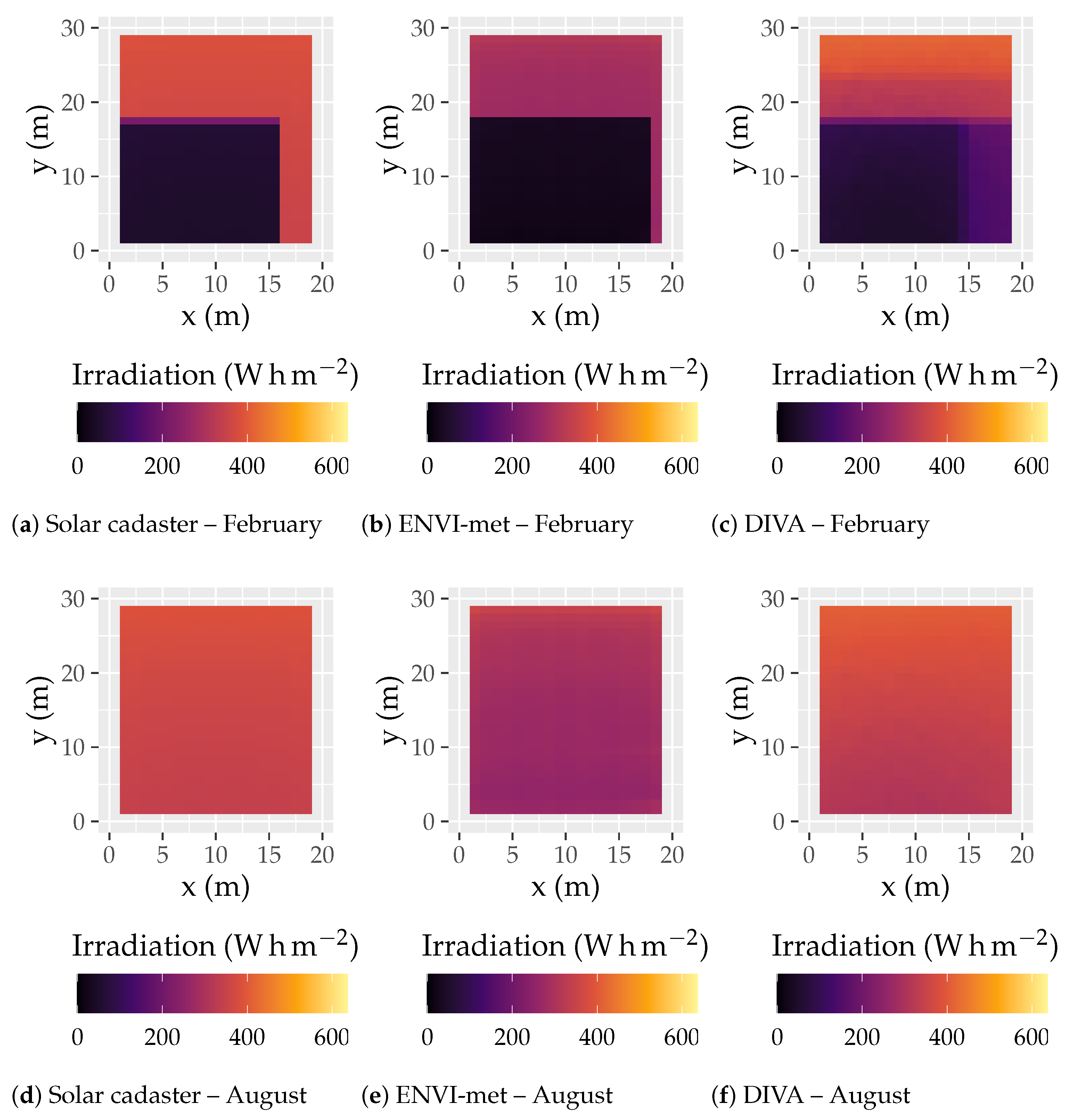
Nevertheless, the level of irradiance on the vertical facades depends on the orientation of the facade, the time of the day, and the time of the year. The levels of irradiance for the south facade of the central building of the homogeneous district are given in Figure 17. Figure 17a–c show the results for the month of February, while Figure 17d–f show the results for the month of August.

Regarding the data, not all are used for comparisons. All of the facades of the buildings are 20 m wide. However, the data at the edges of facades were not analyzed. Indeed, these data are difficult to compare because of the difference in terms of the calculation method for the three tools considered (depending on the tool, irradiance is considered as that at the center of the mesh or as the average over it); see Figure 4. This source of difference, due to the schemes specific to the tools, does not lead to a significant difference in the results, except at the edges of the facades.

The irradiance levels appear to be more homogeneous on the south facade for the month of August than for the month of February. This can be explained by the sun’s higher path at this time of year. The greater range in terms of value (see Figure 15 and Figure 16) is then due to the shading effect, which is more intense in February and leads to a range of irradiance of 50 $\mathrm{W} {\mathrm{m}}^{-2}$ over the south facade in August in comparison with 350 $\mathrm{W} {\mathrm{m}}^{-2}$ in February.

Regarding the level of irradiance predicted by the solar cadaster, which is shown in Figure 17a,d, the values are similar to those predicted by ENVI-met and DIVA-for-Rhino.

Nevertheless, although the predicted irradiance levels are close to each other, there are two particular points. First, the shape induced by the shading is not exactly the same for the solar cadaster and ENVI-met on the one hand and for DIVA-for-Rhino on the other hand. The latter predicts a smoother evolution of the predicted irradiance level. This smoothness is due to the method used for the evaluation of the radiative phenomena; DIVA-for-Rhino uses ray-tracing while ENVI-met and the solar cadaster use the radiosity method. The second point is how the irradiance is evaluated. ENVI-met considers the irradiance to be that at center of the mesh, while DIVA-for-Rhino and the solar cadaster consider it to be the average of the irradiance over the mesh. In the case of DIVA-for-Rhino, it reinforces the smoothness of the evolution of the irradiance over the facade. Concerning the solar cadaster, this has an impact at the edge of the shade (the horizontal purple line at the height of 17 m in Figure 17a).

4. Discussion

The results presented so far show a general good accordance between the three tools considered in terms of both the mean values the irradiance maps. Nevertheless, two points must be noted:

• The prediction of the irradiance is highly sensitive around sunrise and sunset;
• A slight time offset between the results of the different tools seems to be present.

Regarding the sensitivity of the predicted irradiance, the highest discrepancies between the results of the tools appear at the first or the last hour of sunshine (see the north and the west facades in Figure 12). These discrepancies are due to a lack of precision between the calculation of the sun’s path and the level of irradiation. This shift has only a slight incidence on the prediction of the irradiance during the day, but sees its influence strongly increase when the sun is close to the horizon. A sunrise that is predicted too early in the morning results in an overestimation of the predicted irradiance at this time of day, while a sunset predicted too late in the evening results in a peak of the predicted irradiance before the dusk.

Figure 17 shows the existence of a time lag between the three tools studied. Indeed, the shapes of the shadow on the south facade are different among the results of the solar cadaster (Figure 17a), ENVI-met (Figure 17b), and DIVA-for-Rhino (Figure 17c). This offset has only a slight influence on the results. Nonetheless, this impact may increase incrementally, especially early in the morning or late in the evening, as mentioned before (see the north facade in Figure 12).

5. Conclusions

The solar cadaster has proven its ability to provide accurate results in terms of the level of irradiance on both roofs and vertical facades. Indeed, the results predicted by the new version of the solar cadaster developed for Greater Geneva are in good accordance with those predicted by ENVI-met and DIVA-for-Rhino.

Regarding the concordance of the results, the non-shaded horizontal surfaces match almost perfectly. This is not the case for the shaded facades and vertical facades, but the results are very satisfactory. The differences observed between the tools come from the differences between the models in terms of diffuse radiation, the evaluation of reflections, or shading.

Finally, the solar cadaster provides precise results at a low spatial resolution while keeping the computation time low. It ranges from a few hours for the solar cadaster and DIVA-for-Rhino to a few days for ENVI-met. It can therefore be used on a large scale and can prove to be a reliable tool for promoting and intensifying the use of solar energy on the scale of Greater Geneva. However, work is in progress to improve the modeling of reflected components and, thus, the reliability of the tool for more complex geometries.

References

- Loi Fédérale sur la réDuction des éMissions de Gaz à Effet de Serre. 2018. Available online: https://fedlex.data.admin.ch/eli/fga/2018/108 (accessed on 24 June 2021).
- Wiginton, L.; Nguyen, H.; Pearce, J. Quantifying rooftop solar photovoltaic potential for regional renewable energy policy. Comput. Environ. Urban Syst. 2010, 34, 345–357. [Google Scholar] [CrossRef]
- Cellura, M.; Di Gangi, A.; Longo, S.; Orioli, A. Photovoltaic electricity scenario analysis in urban contests: An Italian case study. Renew. Sustain. Energy Rev. 2012, 16, 2041–2052. [Google Scholar] [CrossRef]
- Hachem, C.; Athienitis, A.; Fazio, P. Design of roofs for increased solar potential BIPV/T systems and their applications to housing units. ASHRAE Trans. 2012, 118, 660–676. [Google Scholar]
- Orioli, A.; Di Gangi, A. Load mismatch of grid-connected photovoltaic systems: Review of the effects and analysis in an urban context. Renew. Sustain. Energy Rev. 2013, 21, 13–28. [Google Scholar] [CrossRef]
- Díez-Mediavilla, M.; Rodríguez-Amigo, M.C.; Dieste-Velasco, M.I.; García-Calderón, T.; Alonso-Tristán, C. The PV potential of vertical façades: A classic approach using experimental data from Burgos, Spain. Sol. Energy 2019, 177, 192–199. [Google Scholar] [CrossRef]
- Hachem, C.; Athienitis, A.; Fazio, P. Energy performance enhancement in multistory residential buildings. Appl. Energy 2014, 116, 9–19. [Google Scholar] [CrossRef]
- Hsieh, C.M.; Chen, Y.A.; Tan, H.; Lo, P.F. Potential for installing photovoltaic systems on vertical and horizontal building surfaces in urban areas. Sol. Energy 2013, 93, 312–321. [Google Scholar] [CrossRef]
- Vulkan, A.; Kloog, I.; Dorman, M.; Erell, E. Modeling the potential for PV installation in residential buildings in dense urban areas. Energy Build. 2018, 169, 97–109. [Google Scholar] [CrossRef]
- Desthieux, G.; Carneiro, C.; Camponovo, R.; Ineichen, P.; Morello, E.; Boulmier, A.; Abdennadher, N.; Dervey, S.; Ellert, C. Solar Energy Potential Assessment on Rooftops and Facades in Large Built Environments Based on LiDAR Data, Image Processing, and Cloud Computing. Methodological Background, Application, and Validation in Geneva (Solar Cadaster). Front. Built Environ. 2018, 4, 14. [Google Scholar] [CrossRef]
- Kajiya, J.T. The Rendering Equation. SIGGRAPH Comput. Graph. 1986, 20, 143–150. [Google Scholar] [CrossRef]
- Sillion, F.X.; Puech, C. Radiosity and Global Illumination; Morgan Kaufmann Publishers Inc.: San Francisco, CA, USA, 1994. [Google Scholar]
- Freitas, S.; Catita, C.; Redweik, P.; Brito, M. Modelling solar potential in the urban environment: State-of-the-art review. Renew. Sustain. Energy Rev. 2015, 41, 915–931. [Google Scholar] [CrossRef]
- Desthieux, G.; Carneiro, C.; Susini, A.; Abdennadher, N.; Boulmier, A.; Dubois, A.; Camponovo, R.; Beni, D.; Bach, M.; Leverington, P.; et al. Solar cadaster of Geneva: A decision support system for sustainable energy management. In From Science to Society; Springer: Berlin/Heidelberg, Germany, 2018; pp. 129–137. [Google Scholar]
- Iqbal, M. An Introduction to Solar Radiation; Academic Press: Toronto, ON, Canada; New York, NY, USA, 1983. [Google Scholar]
- Stendardo, N.; Desthieux, G.; Abdennadher, N.; Gallinelli, P. GPU-Enabled Shadow Casting for Solar Potential Estimation in Large Urban Areas. Application to the Solar Cadaster of Greater Geneva. Appl. Sci. 2020, 10, 5361. [Google Scholar] [CrossRef]
- Reinhart, C.F.; Andersen, M. Development and validation of a Radiance model for a translucent panel. Energy Build. 2006, 38, 890–904. [Google Scholar] [CrossRef]
- Perez, R.; Seals, R.; Michalsky, J. All-weather model for sky luminance distribution—Preliminary configuration and validation. Sol. Energy 1993, 50, 235–245. [Google Scholar] [CrossRef]
- Tregenza, P.R. Subdivision of the sky hemisphere for luminance measurements. Light. Res. Technol. 1987, 19, 13–14. [Google Scholar] [CrossRef]
- Reinhart, C.F.; Herkel, S. The simulation of annual daylight illuminance distributions—A state-of-the-art comparison of six RADIANCE-based methods. Energy Build. 2000, 32, 167–187. [Google Scholar] [CrossRef]
- Perini, K.; Chokhachian, A.; Dong, S.; Auer, T. Modeling and simulating urban outdoor comfort: Coupling ENVI-Met and TRNSYS by grasshopper. Energy Build. 2017, 152, 373–384. [Google Scholar] [CrossRef]
- Kolokotsa, D.D.; Giannariakis, G.; Gobakis, K.; Giannarakis, G.; Synnefa, A.; Santamouris, M. Cool roofs and cool pavements application in Acharnes, Greece. Sustain. Cities Soc. 2018, 37, 466–474. [Google Scholar] [CrossRef]
- Farhadi, H.; Faizi, M.; Sanaieian, H. Mitigating the urban heat island in a residential area in Tehran: Investigating the role of vegetation, materials, and orientation of buildings. Sustain. Cities Soc. 2019, 46, 101448. [Google Scholar] [CrossRef]
- Govehovitch, B.; Giroux-Julien, S.; Gaillard, L.; Peyrol, E.; Ménézo, C. Numerical and experimental study of two PV power generation models for buildings façades. Solar World Congress/ISES Conference Proceedings. 2019. Available online: http://proceedings.ises.org/paper/swc2019/swc2019-0182-Govehovitch.pdf (accessed on 24 June 2021).
- Bruse, M.; The ENVI-Met Team. Advances in Simulating Radiative Transfer in Complex Environments. Available online: https://www.envi-met.com/wp-content/uploads/2020/11/201119-530_06_201116-CaseStudy_IVS-1-1.pdf (accessed on 24 June 2021).
- Cheng, V.; Steemers, K.; Montavon, M.; Compagnon, R. Urban Form, Density and Solar Potential. In Proceedings of the 23rd Conference on Passive and Low Energy Architecture, Geneva, Switzerland, 6–8 September 2006. [Google Scholar]
- Natanian, J.; Aleksandrowicz, O.; Auer, T. A parametric approach to optimizing urban form, energy balance and environmental quality: The case of Mediterranean districts. Appl. Energy 2019, 254, 113637. [Google Scholar] [CrossRef]
- Lobaccaro, G.; Fiorito, F.; Masera, G.; Poli, T. District Geometry Simulation: A Study for the Optimization of Solar Façades in Urban Canopy Layers. Energy Procedia 2012, 30, 1163–1172. [Google Scholar] [CrossRef]
Figure 1.
Illustration of backward and forward ray tracing.
Figure 2.
Illustration of specular and diffuse reflection.
Figure 3.
Shadow casting of the solar cadaster, adapted with permission from [
10,
14].
Figure 4.
Differences in terms of irradiance calculations for a mesh.
Figure 5.
Geometry used for the study of the influence of the mesh.
Figure 6.
Cumulative irradiation for different mesh resolutions.
Figure 7.
Sketch of the homogeneous neighborhood.
Figure 8.
Sketch of the heterogeneous neighborhood.
Figure 9.
Shortwave radiation used as input.
Figure 10.
Spatial average of the irradiance received on the unshaded roofs (homogeneous neighborhood or buildings 6 and 7 of the heterogeneous neighborhood).
Figure 11.
Spatial average irradiance received on the facades for the homogeneous district in February.
Figure 12.
Spatial average irradiance received on the facades for the homogeneous district in August.
Figure 13.
Spatial average irradiance received on the facades in the heterogeneous district in February.
Figure 14.
Spatial average irradiance received on the facades in the heterogeneous district in August.
Figure 15.
Distribution of the irradiance over the vertical facades for the homogeneous district in February.
Figure 16.
Distribution of the irradiance over the vertical facades for the homogeneous district in August.
Figure 17.
Irradiance map of the homogeneous district for the south facade over 12 h.