Quantification of the Information Loss Resulting from Temporal Aggregation of Wind Turbine Operating Data

Abstract

SCADA operating data are more and more used across the wind energy domain, both as a basis for power output prediction and turbine health status monitoring. Current industry practice to work with this data is by aggregating the signals at coarse resolution of typically 10-min averages, in order to reduce data transmission and storage costs. However, aggregation, i.e., downsampling, induces an inevitable loss of information and is one of the main causes of skepticism towards the use of SCADA operating data to model complex systems such as wind turbines. This research aims to quantify the amount of information that is lost due to this downsampling of SCADA operating data and characterize it with respect to the external factors that might influence it. The issue of information loss is framed by three key questions addressing effects on the local and global scale as well as the influence of external conditions. Moreover, recommendations both for wind farm operators and researchers are provided with the aim to improve the information content. We present a methodology to determine the ideal signal resolution that minimized storage footprint, while guaranteeing high quality of the signal. Data related to the wind, electrical signals, and temperatures of the gearbox resulted as the critical signals that are largely affected by an information loss upon aggregation and turned out to be best recorded and stored at high resolutions. All analyses were carried out using more than one year of 1 Hz SCADA data of onshore wind farm counting 12 turbines located in the UK.

1. Introduction

In modern wind turbines, a plethora of operating data are acquired with high temporal frequency [1,2] by a vast number of sensors [3,4]. However, usually only a selection of these sensor data is stored. Furthermore, the data are typically aggregated as 10-min average values, sometimes accompanied by the standard deviations or the maxima and minima measured in these intervals. This temporal aggregation of a signal, also referred to as downsampling, saves a lot of space upon storage and reduces the bandwidth needed when transferring the data, both connected to cost savings. Unfortunately, much of the information on short timescales that might be valuable to better model and track the behavior and condition of wind turbines is inevitably lost in this process [4,5,6].

Aggregating data induces an information loss regardless of the source of data, even though its impact depends on the downsampling rate with respect to the behavior and the resolution of the raw signal. Albeit, the consequences arising from this signal conversion depend strongly on the further use of the data. Understanding these consequences, by knowing the properties of a signal after its transition to lower resolutions, will therefore help to optimize both data storage and costs while at the same time providing the best possible signal quality for analytic investigations.

In this study we investigate operating data of wind turbines recorded by the supervisory control and data acquisition system (SCADA). SCADA is a control system which among other functionalities allows for monitoring of wind turbines and receives input from a net of sensors that measure various operating variables such as wind speed, active power, temperatures, pressures, speeds, and environmental conditions through time. As we only investigate operating data, we will refer to “SCADA operating data” as simply “SCADA data” throughout the paper. Please note that although we developed the methods and algorithms to quantify information loss for wind turbine data, they are not necessarily restricted to our use case. While the considerations regarding specific consequences are limited to the wind energy field only, the approach can also be extended to other fields of application.

In many technological sectors data are considered a key asset to foster growth and innovation—wind energy is no exception. In the need of clean energy, wind power prospers globally: During the year 2020, 111GW of new capacity were installed worldwide [7]. In Europe alone, wind power capacity amounted to 220GW by the end of 2020. It is desired to grow between 80 and 105GW over 2021–2025 out of which 29GW are planned to be installed offshore [8]. Therefore, using data for better and more efficient operational strategies will be pivotal to further reduce the costs and to sustain the competitiveness of wind production compared to conventional energy sources. On the one hand, a profound data basis can support methods for accurate power output predictions. An overview about possible wind energy forecasts was given by Okumus and Dinler [9]. On the other hand, monitoring the health status of turbines supports the improvement of reliability by understanding and anticipating failures. The current state of using SCADA data for condition monitoring was summarized by Tautz-Weinert and Watson [4]. Each prevented turbine fault will avert a subsequent standstill and an involved loss of revenue. In the end this also reduces the costs for operation and maintenance (O&M) that currently account for up to 30% of an onshore wind turbine’s levelized cost of electricity (LCOE) and up to 25% of the much higher LCOE of an offshore turbine [10]. These costs are thus still a major burden for the wind energy industry.

Research can help to minimize such costs by approaches of early fault detection or health monitoring methods. One possible solution addresses mechanical components by monitoring, e.g., the drivetrain or transmission elements through rich high-frequency data. Typically the sensors used are not part of the standard equipment of a turbine but of a dedicated condition monitoring system (CMS). Therefore, such a system needs to be installed explicitly and this is associated with further costs [11]. Occasionally, such high-resolution operating data are—partly—available from SCADA systems and could be used for the same purpose.

As stated earlier, data storage and transfer are associated with expenses. Therefore, for a cost optimization it is necessary to find a trade-off between reducing the amount of data, i.e., signal scope or resolution, and retaining enough information content to support O&M strategies. To illustrate the information loss Figure 1 shows the outcome of temporal aggregations of SCADA data at different time resolutions. Large aggregation intervals in the order of 300 to 600 s are not able to capture all nuances of the signal as local minima and maxima are flattened in the mean value curves. Clearly, this is only an example obtained for the wind speed and one temperature of the transmission shaft bearings, but similar behaviors can be observed for all signals.

Nevertheless, the figure gives an idea of the possible effects of temporal aggregation. A thorough study of the phenomena of information loss due to temporal data aggregation in the context of wind turbine SCADA data will be presented throughout this paper. The objective is to provide a deep analysis of the crucial points when aggregating SCADA data and to quantify the span of the information loss phenomenon. We also want to support turbine operators with a framework that allows them to take better decisions in terms of SCADA data storage and aggregation policies. We break the general motivation down into these three specific research questions:

• Q1: How much information is lost with reduced temporal resolution?
• Q2: Do external conditions have an effect on information loss?
• Q3: What is the recommended aggregation frequency?

This paper is structured as follows: Section 2 provides a review of related work dealing with wind turbine monitoring and the use of high-frequency data in wind and other application sectors. Section 3 details the data set used in this study. Then, Section 4 tackles the key questions of this paper. Each subsection guides through our analytical approaches to answer these question and the corresponding results obtained. A discussion of the salient points derived from this study is also included for each question. Finally, Section 5 draws conclusions and discusses limitations of the study, the most relevant information, and ideas for future work.

2. Previous Work

Studies in the wind energy sector using high-frequency SCADA data are still scarce as these data sets are rare. Industry practice and state of the art is using aggregated SCADA operating data as 10-min averages. Nonetheless, a few available publications show the potential of the utilization of high-frequency SCADA data [1,2,12,13,14,15].

Generally SCADA data can be used for a high variety of applications. Two examples for major tasks in the wind energy sector are the prediction of the power output and the assessment of the turbine or component health status. Both problems are crucial for wind power production as they allow wind farm owners to keep their turbines spinning more and reduce mismatches between promised and delivered energy.

Power production estimation is a very large field of study within wind energy. A wide array of methods are available to predict power output [16,17,18]. The approaches vary on the type of data that is fed to the algorithms as well as the strategy used to detect patterns in the data. SCADA data was used in Refs.  [15,19]. Since there is typically at least both the wind speed and the generated power within the SCADA data set, power output could ideally be estimated directly. However, this proved to be a very challenging task. Physical models focus mostly on the accurate prediction of the wind speed [20,21]. By using the characteristic power curve of a turbine, it is then translated to a modelled power.

As various models base on SCADA data and the resolution of this data is usually 10 min, i.e., rather low, it is relevant to determine the limitations of such aggregated data to better understand the possible shortcomings when predicting the power output. Gonzalez et al. discussed the advantages of using high-frequency SCADA data in conjunction with a quantile random forest as predictive maintenance tool based on power curve modeling. The SCADA data used had a resolution of 4 s and was utilized to compare the predicted performance with 10-min averaged signals. As the natural variability of turbine operation was better captured by the high-frequency data, it also resulted in improved predictions [13]. In a later study, the same authors conducted a sensitivity study on the performance of high-frequency SCADA data as performance monitoring tool. Various factors such as terrain complexity, seasonality, choice of input variable, and most relevantly the sampling rate of data were analyzed. An important conclusion was the observation that a higher resolution allows to create more reliable models and as a key take-away they proposed to determine how much of the dynamic behavior of the signal is lost due to averaging [2]. Furthermore, the frequency of SCADA data is important to correctly model wake effects in wind farms. An inaccurate evaluation of wakes leads to imprecision in estimating wind speed and subsequent turbulence, which ultimately results in a poor prediction of power output [22].

A second important aspect in turbine operation is predictive maintenance. Unexpected and sudden failures can be very expensive for turbine owners and, therefore, an assessment of the turbine or component status shows up beneficial. The available data, the monitored system, and the requirements greatly influence the design and choice of a predictive maintenance toolbox.

As previously mentioned the drivetrain and other mechanical components, such as bearings and shafts, can be monitored by measuring acceleration, displacement and vibration through specific sensors and via acoustics emissions by dedicated CMS [11]. Additionally, for electrical and electronic components it is possible to apply CMS by analyzing current signatures in search of anomalous patterns [23]. These approaches are all based on utilization of very rich data, characterized by high sampling rates in the order of kHz. Here, signal processing techniques such as Fast Fourier transform, Hilbert–Huang transform, or wavelets analysis can be adopted [24,25,26,27].

Nonetheless, alternatives to the implementation of dedicated CMS in a wind turbine exist. SCADA data, while available at a much lower frequency and far poorer in terms of information, has also proven as a valid and cheap instrument for turbine monitoring. A short investigation on the usability of high-frequency SCADA data for predictive maintenance has been carried out by Roberts et al. [14]. In order to obtain the condition of a turbine, a quite plain approach is to model the power output and compare it to its measured value. In this manner, defects can be detected—ybut not localized—when significant discrepancies are observed [28,29]. So-called normal behavior models are another popular mathematical approach. These are regression models designed to predict the value of a key variable, capable of capturing the status of the studied system. A set of input variables is fed to an algorithm and the difference between the predicted and measured value is tracked. Large deviations are marked as anomalies and can be inspected further [30]. This goal can, e.g., be pursued by physical models [31] or neural networks [32]. Alternative approaches based on anomaly detection and fusion of multiple indicators and alarm logs, addressing generator and main bearing failures, have been proposed in [33,34]. When located in a wind farm, also adjacent turbines can serve as a reference value [31].

Further research also investigated simulating load by means of SCADA data from a single turbine or even the farm [35,36], eventually serving as an input for residual useful lifetime (RUL) estimations. Using the data of a whole farm can also serve to reconstruct an optimized flow through the area of this farm [37].

Dealing with the loss of information when temporally aggregating data or reducing the sampling rate is not an issue that occurs exclusively in wind energy. Nowadays, in cars even more data is collected by their electronic control units. Processing these data faces a similar problem: Liu et al. investigated the effects of reducing the sampling rate of the driving data with a particular focus on so-called micro-driving decisions such as spontaneous accelerations [38]. One result of this highly dynamic behavior was that the amount of information does not decrease linearly when reducing the temporal resolution, but that there are resolution ranges where no further information is lost whereas it falls down rapidly for other ranges.

Having considered the state of the art regarding wind turbine monitoring and power prediction, this paper aims to advance the understanding of information loss and possible limitations of SCADA data. In particular, the effect of low temporal resolution is analyzed and a quantitative method to determine the amount of lost information is detailed. Using this framework it is possible to determine signals that are most affected by downsampling and identify the influence of seasonal behavior and differences between turbines. An analysis of the effect of wind speed on information loss is also discussed, determining which operating conditions are affected the most by information loss. Finally, a methodology to choose an optimal aggregation frequency for a given signal is presented allowing to minimize the data storage footprint, while retaining most of the relevant information. In comparison with other high-frequency investigations this research offers the advantage of a large dataset consisting of more than one year of 1 Hz operating data that supports our conclusions.

3. Data

In this research we consider operating data generated by the SCADA system of wind turbines. The data set is gathered from an onshore wind farm consisting of 12 turbines with a nominal power of 2MW commissioned in 2017 and located in the UK. The investigated period covers 15 months of data collection, hence seasonality effects should be limited.

Various signals that measure and monitor operational and ambient conditions are available with a temporal resolution of 1 second. Signals that represent counters are excluded in this analysis. In total, 27 signals are evaluated including temperatures, pressures, speeds, voltages, currents, and pitch angles.

Table 1. List of SCADA signals analyzed in this study.

Component	Control	Electrical	Environmental	Mechanical
Temperatures	Variables	Characteristics	Variables	Characteristics
Generator bearing 1	Pitch angle blade 1	Active power	Ambient temperature	Generator speed
Generator bearing 2	Pitch angle blade 2	Current phase A	Nacelle temperature	Rotor speed
Generator stator	Pitch angle blade 3	Current phase B	Wind direction
Gearbox oil	Yaw angle	Current phase C	Wind speed
Gearbox shaft bearing 1		Grid frequency
Gearbox shaft bearing 2		Power factor
Main bearing		Voltage phase A
Top box		Voltage phase B
		Voltage phase C

provides an overview of the investigated signals, partitioned into functional groups. Please note that in this study only operating data is considered.

The time stamps of the original dataset are not always exact to the tick of a second. Sensors, for various reasons, might record their values slightly early or late. For computational reasons we decided to adjust the timestamp downward to seconds with the typical floor-functions available. Therefore, in a few cases two different records were assigned to the same timestamp. In these cases only the earlier one of the two values is kept. Furthermore, for missing data no replacement, i.e., no imputation, was performed and generally no treatment for outliers was performed, except for the descriptive statistics in Section 4.1.1.

In order to examine the effect of temporal aggregation, throughout this paper downsampling of high-resolution data to a lower temporal resolution is accomplished by averaging if not stated otherwise.

Table 2. Illustration of the temporal aggregation scheme: The original data, i.e., t (1 s), is averaged over the lower temporal range and given a new timestamp at the beginning of this interval, see t (5 s) and t (10s).

t (1 s)	Wind Speed (m/s)	t (5 s)	Wind Speed (m/s)	t (10 s)	Wind Speed (m/s)
09:00:00	6.26	09:00:00	6.25	09:00:00	6.42
09:00:01	6.11
09:00:02	6.17
09:00:03	6.39
09:00:04	6.32
09:00:05	6.37	09:00:05	6.71
09:00:06	6.66
09:00:07	6.72
09:00:08	6.72
09:00:09	7.07
09:00:10	7.29	09:00:10	...	09:00:10	...

depicts an example for the temporal aggregation of the wind speed.

4. Analyses

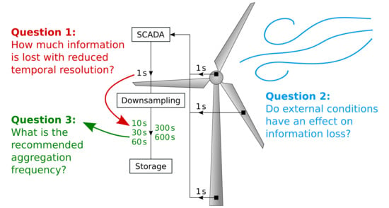
In this section, we present the applied methods addressing each research question Q1–Q3. Furthermore, the corresponding results are reported, described, and discussed.

4.1. Q1: How Much Information Is Lost with Reduced Temporal Resolution?

Understanding the effect of temporal aggregation, quantifying the induced information loss, and identifying the signals which are affected the most are important steps to find a trade-off between data volume and information content. Hence, storage policies can be defined and possibly additional space can be allocated for the signals that are not recommended for aggregation. The methods and approaches in this subsection address the guiding question, if data when sampled at a higher frequency contains richer information. In this study simple approaches based on statistics indicators and tests are replicated. Then, given their limitations a different method based on the analysis of the aggregation error is devised.

4.1.1. Comparison of Descriptive Statistics

The effect of different levels of aggregation of data is studied by comparing the values of a set of descriptive statistics. The objective is to identify global changes in the signals that are reflected in their range, central behavior and overall shape of distribution.

Methodology

 

In order to evaluate the effects of temporal aggregation, the first approach constituted the calculation of key descriptive statistics, which captured the central behavior, shape and dispersion of the data. To examine the effect of temporal aggregation, these statistics were computed for the non-aggregated, i.e., raw data (1 second of temporal resolution) and for temporally aggregated data with reduced time resolutions, namely 10 s, 60 s, 300 s, and 600 s. For each signal listed in Table 1 the following statistics were computed for all resolutions mentioned above: sample mean, median, maximum, minimum, standard deviation, first quartile, third quartile, skewness, and kurtosis. For the calculation specification of these quantifiers we refer to Ref.  [39].

In contrast to the subsequent analyses, the calculations of this part were carried out on the entire dataset. To keep extreme outliers out of the scope for less distorted results, during this analysis the data for wind speed and generator speed were filtered for only positive values and temperatures for values < 200 °C.

Results

 

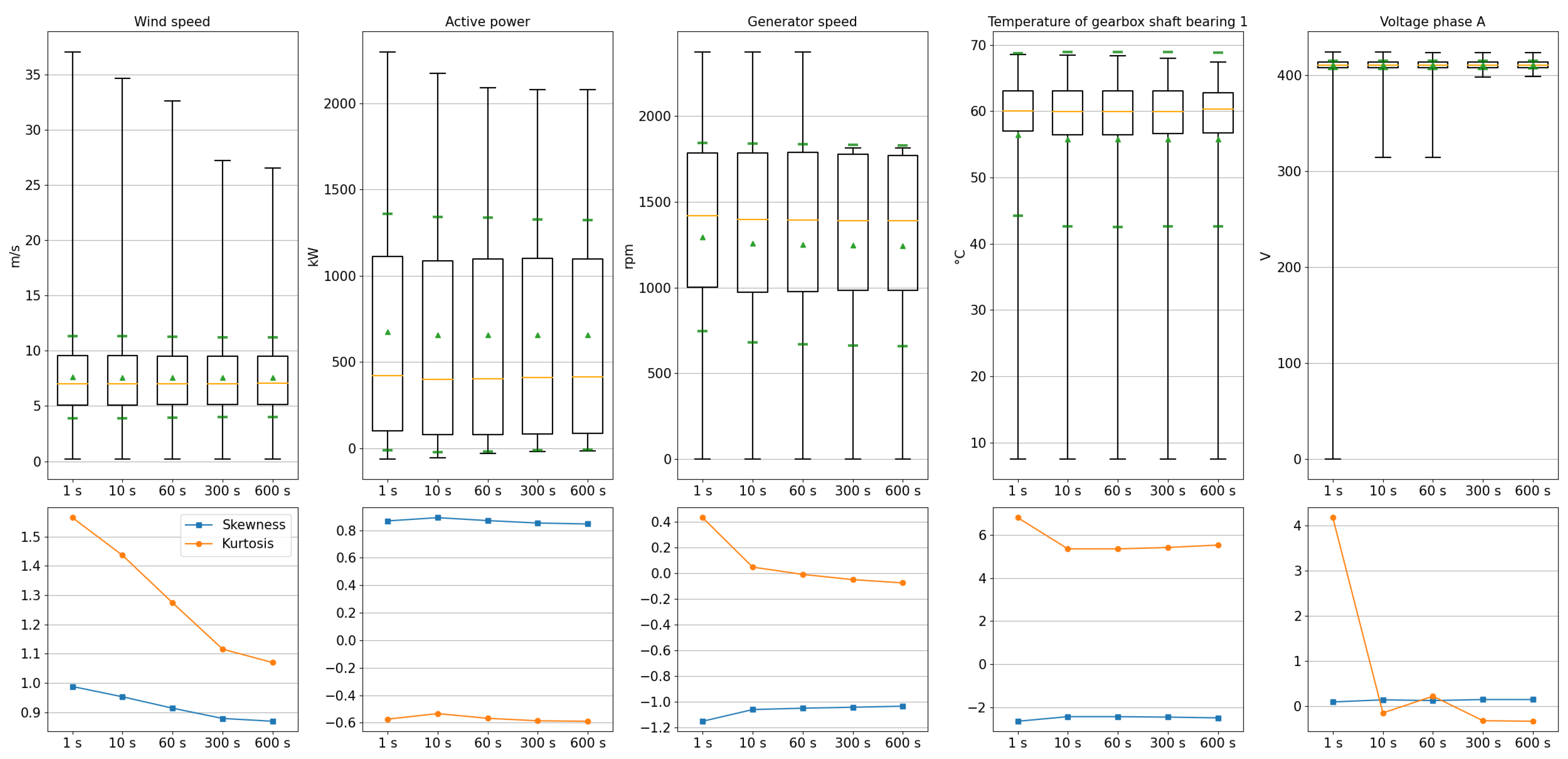
Selected results are shown in Figure 2 for one turbine. The full list of computed statistics based on different temporal resolutions for the entire set of signals is provided in the Supplementary Materials. Here, we present an appropriate graphical representation using a box-and-whisker-plot [40], which includes the mean (denoted by the green triangles), the median (denoted by a horizontal yellow bar in the box), the first quartile (denoted by the bottom edge of the box), the third quartile (denoted by the top edge of the box), the minimum (denoted by the bottom edge of the whisker) and the maximum (denoted by the top edge of the whisker). Moreover, the green bars in the plot represent the mean value ± the standard deviation. These are shown for four exemplary signals, namely wind speed, active power generation, generator speed, one temperature of the gearbox shaft bearings, and the voltage of phase A. Note that in this version of box-and-whisker-plots the whiskers represent the minimum and maximum of the underlying data and therefore include outliers.

To display the results of skewness and kurtosis we chose a simple scatter plot that is displayed in the second row of Figure 2 for the same signals mentioned above accordingly. As both measures are normalized to the standard deviation they are both plotted against the same dimensionless ordinate.

From the representative statistics of the graphical presentation in Figure 2 and the additional data in the Supplementary Materials the following results can be obtained:

• Temporal aggregation had a pronounced effect on the maxima: with lower temporal resolution the maxima decreased. Especially for the wind speed we saw a distinct decreasing trend of the maxima (for this presented turbine and investigated time period a reduction of 10 m/s).
• A corresponding effect for the minima, i.e., an increasing trend, could not be seen for those variables with a defined lower boundary, e.g., 0 m/s for the wind speed. Here, lower boundaries were preserved. For other variables, a similar but much less pronounced effect was existent, e.g., for the active power generation. The one exception was the voltages, as their value only dropped from the reference value in the case of disturbances.
• Mean and median faintly declined for most signals with increasing temporal aggregation, though in the illustration no noticeable visual differences could be obtained.
• The standard deviation and the interquartile range (IQR) behaved similarly, although both also experienced only small changes: For some values they faintly decreased, e.g., for the wind speed and the active power, whereas for others like generator speed and the temperature of the gearbox shaft bearings they made a small increasing step between 1 s and 10 s.
• The values of skewness were rather close to each other for different levels of temporal aggregation. Although the base values scattered a lot, the median of their changes for all turbines and signals lay below 5% with respect to the raw signal. An explicit decline could only be seen for the wind speed.
• For the kurtosis a clear trend could only be observed for the wind speed and the voltages where there was a clear decline with increasing temporal aggregation. For the rest of the signals this was not as clear: for several signals there was almost no difference, some signal tended to increase for one turbine, but decreased for another. However, the median of all changes lay below 5% change in standard deviation with respect to its value at 1 s resolution.

In summary, the statistics of typically fast changing signals such as wind speed, active power, generator speed, and electrical signal were the most affected by downsampling as the values of their statistics varied widely with the resolution of the signal. Temperature signals, on the other hand, were far less affected by downsampling.

Discussion

 

Most prominent variations in the statistical analysis are the minima and maxima of the signals, displayed by the whiskers in Figure 2. Mostly, maxima tend to decrease with the length of the aggregation period, meaning that longer aggregations smooth out peak values of the signal possibly annihilating anomalous conditions. If peak values are strongly reduced from the data, it can be assumed that also short negative spikes will undergo the same behavior. Except for the voltages, this cannot be seen in most plots as the minima coincide with those periods in which turbines are not operating. Still, this reduction of peak values might negatively impact the possible performance of early-fault detection algorithms and more general models attempting to represent the behavior of turbines under peak load conditions. For these use cases, high frequency SCADA should be considered.

Mean and median values are almost constant with respect to the aggregation period length as the total weight of the values cannot be significantly shifted by averaging. The change of the standard deviation and the IQR behaves differently and can exhibit the following patterns: An increase means that several sudden outliers on short timescales are annihilated by the averaging process and, therefore, less data is distributed at the tails. A decrease is observed when the values move to the tails by the averaging process due to the majority of data inside an aggregation windows distributed at the tails.

The shape indicators skewness and kurtosis do not provide completely conclusive information. However, there seems to be a connection between the reduction of the maximum or minimum and a decrease of the kurtosis, as can be seen for the wind speed, the generator speed, and the voltage. If due to the aggregation process there are less remote outliers, the probability distribution of the data becomes less spiked. Consequently, we can observe a loss of short-time peaks in the data by the reduction of the kurtosis. In contrast, the interpretation of the skewness is not as simple. However, it should give a hint to the direction of the majority of outliers or peaks, respectively. For the wind speed the skewness becomes less negative, telling us, that most of the outliers in the positive direction for the 1 s data will be smoothed out with increasing aggregation time. For the generator speed of the exemplary turbine in Figure 2 more outliers from the negative direction are smoothed. Please note again, that these are not generally valid as, except for the wind speed, the behavior of the skewness of a signal varies from turbine to turbine in the given dataset.

Observing the behavior of a set of descriptive statistics provides a simple check on the effect of temporal aggregation. The proposed analysis attempts to capture various characteristics of the signal distribution, including its shape, dispersion, and central behavior. Overall, this observation of descriptive statistics does not answer the question on how much information is lost due to temporal aggregation. Changes in the range and standard deviation of the signals provide a general indication of the effects of temporal aggregation for a set of signals. Although pointing at the temporally critical signals, they fail to quantify precisely the loss of information. Moreover, this approach does not provide insights into the dynamic behavior of the signals as all indicators provide only a global perspective. Providing indications on the optimal frequency of a signal based on the value of descriptive statistics is particularly challenging.

4.1.2. Kolmogorov–Smirnov Test

Beside comparing descriptive statistics calculated for different levels of aggregation, inferential methods were applied in order to quantify a change of the distribution of the aggregated signal. Here, the Kolmogorov–Smirnov (KS) two sample test was used to ascertain whether the distribution of the temporally aggregated signal differed from the distribution of the non-aggregated signal.

Methodology

 

We only briefly introduce the idea and procedure of the test, for a detailed description please see [41].

In this work, the KS two sample test was applied and no assumption on the distribution of the underlying data was made. Suppose the data consisted of two independent samples, a first sample $X_1,X_2,...,X_n$ of size n and a second sample $Y_1,Y_2,..,Y_m$ of size m. $F\left(x\right)$ and $G\left(x\right)$ denote their respective, unknown distribution functions. We wanted to test the hypothesis

$$H_0:F\left(x\right)=G\left(x\right)\mathrm{vs}.H_1:F\left(x\right)\ne G\left(x\right).$$

(1)

Let $F_n\left(x\right)$ be the empirical distribution function based on the random sample $X_1,X_2,...,X_n$ and let $G_m\left(x\right)$ be the empirical distribution function based on the random sample $Y_1,Y_2,..,Y_m$. Then, the test statistic D measures the maximum difference between the two empirical distribution functions and is defined as

$$D=\underset{x}{sup}|F_n\left(x\right)-G_m\left(x\right)|.$$

(2)

From the test statistic D the p-value was derived, adjusting for the different sample sizes n and m. As a level of significance the typical value of $\alpha$ = 0.05 was chosen.

If the p-value was smaller than the level of significance, i.e., $p<0.05$, $H_0$ was rejected and we had sufficient evidence to say the aggregated data had another underlying distribution. If the p-value was greater than 0.05, then we did not have sufficient evidence to reject the null hypothesis and we could not draw any further conclusions. Please note that in our case there was an important difference of the test application when compared to its standard use. Here, we compared two samples that are known to come from the same generating process, as the tested signal was the same. Therefore, the test tried to determine whether the aggregation process changed the distribution of the signal such that the aggregated and original distribution no longer appeared similar.

Results

 

The test statistics D and the p-values were calculated for all signals based on incorporating the raw signal and several aggregated signals on different temporal resolutions of 10 s, 60 s, 300 s, and 600 s, equivalent to Section 4.1.1. The test was conducted with 10,000 h of randomly chosen samples of operating data. As the quantity of interest we present the derived p-values for an exemplary turbine, i.e., turbine 5, containing all investigated signals on the left side of Figure 3 and the minimum values of all turbines on the right. Data containing all numerical results are provided in the Supplementary Materials.

Regarding all turbines the majority of p-values for all signals were above the significance level of 0.05. Especially for higher resolutions < 60 s the p-values even tended to keep around 1, making it very unlikely that both the raw and aggregated value came from two different underlying distributions. There was even a set of signals whose p-values were always 1. These were the active power generation, grid frequency, generator speed, all pitch angles, power factor, and rotor speed. The turbine on the left of the figure had explicitly been chosen because it featured p-values below 0.05 for certain channels for aggregated data of 600 s resolution. As displayed on the right of Figure 3, regarding the whole wind farm for the following signals the KS test showed p-values below 0.05 at least for one turbine: the temperature inside nacelle ($1\times$), both generator bearing temperatures as well as the generator stator temperature (each $1\times$), the top box temperature ($1\times$), voltage phase B ($1\times$), wind direction ($2\times$), wind speed ($2\times$), and yaw angle ($1\times$). Thus, for the last mentioned group of signals, resampling to 600 s could alter the data in a way such that the underlying distribution of the data was no longer the same as for the raw data. One additional signal that also came close to our significance level with a p-value of 0.082 once within the scope of all turbines was the ambient temperature.

Discussion

 

From the results of all turbines, we extracted the minimum p-value for each signal and aggregation value in Figure 3. Of course, this is a rather unconventional approach with questionable statistical significance. Nevertheless, in this way the results of the KS test can be divided into three signal subgroups that are shown in

Table 3. Signals sorted into bins of $p_{\min }$. Here, $p_{\min }$ is the minimal p-value of a signal for all aggregation resolutions and turbines as already carried out in Figure 3.

${\mathit{p}}_{\mathbf{min}}\ge 0.98$	$0.98>{\mathit{p}}_{\mathbf{min}}\ge 0.05$	${\mathit{p}}_{\mathbf{min}}\le 0.05$
Active power	Ambient temperature	Temperature inside nacelle
Generator speed	Current phase A	Temperature of generator bearing 1
Grid frequency	Current phase B	Temperature of generator bearing 2
Pitch angle blade 1	Current phase C	Temperature of generator stator
Pitch angle blade 2	Temperature of gearbox oil	Top box temperature
Pitch angle blade 3	Temperature of gearbox shaft bearing 1	Voltage phase B
Power factor	Temperature of gearbox shaft bearing 2	Wind direction
Rotor speed	Temperature of main bearing	Wind speed
	Voltage phase A	Yaw angle
	Voltage phase C

: (1) signals for which the test yields p-values of 1 or only slightly below. (2) Signals with a resulting p-value that decreases with increasing aggregation time, but never falls below the chosen level of significance of 0.05. (3) Signals that fall below the level of significance at least once for all turbines.

For the first group of signals the p-value of the KS test was always much higher than our level of significance of 0.05, some even stayed permanently at 1. Although, from these results we can only conclude that the two samples, i.e., the raw data and the aggregated values, are not from two different underlying distributions, it is also a good sign, because it gives us an indication that most of the aggregated signals are not strongly disturbed with respect to the original signal for all resolutions. Other signals showed a decreasing p-value with increasing aggregation time. Still, most of the p-values were above our significance threshold. This could mean that, contrary to the first group, the signals deviate more and more with when decreasing the resolution. In the third group of signals, the KS test resulted in p-values below the level of significance at least once for all turbines. These low values of $p<0.05$ occurred only for aggregation times of 600 s and only once or twice in the whole set of turbines. Therefore, they do not tell us that the respective signals are always altered heavily by the aggregation process. However, those data give us hints to signals that can show short term deviations in their time series that might be annihilated during mean value aggregation process. Therefore in return, these short term deviations only occur very rarely—in our case only for one or two turbines. Regarding the voltages, there was even only one prominent phase. The observed rarity also makes it hard to tell that the list of signals with eventual important short term deviations is complete. For example: All voltages should behave in the same manner.

As a conclusion, the KS test revealed deviations for signals of which some fall into a group of typically fast changing values, such as the wind speed and direction, and the measured voltages. The other group consists of some rather lagged signals with several temperatures as well as the yaw angle. These signals might contain valuable information on short timescales that is lost during aggregation while it might serve as an important input for future predictive methods such as early fault detection. Finding these short-time features will certainly be a task for the learning process of such methods. Here, the KS test might be helpful to identify the interesting signals and time ranges. However, the KS test falls short of giving quantifiable indications on which resolution to choose.

4.1.3. Local Error Approach

In this section we will address the information loss directly, conducting an analysis on the bare differences between the raw signal and the signals aggregated over different aggregation intervals.

Methodology

 

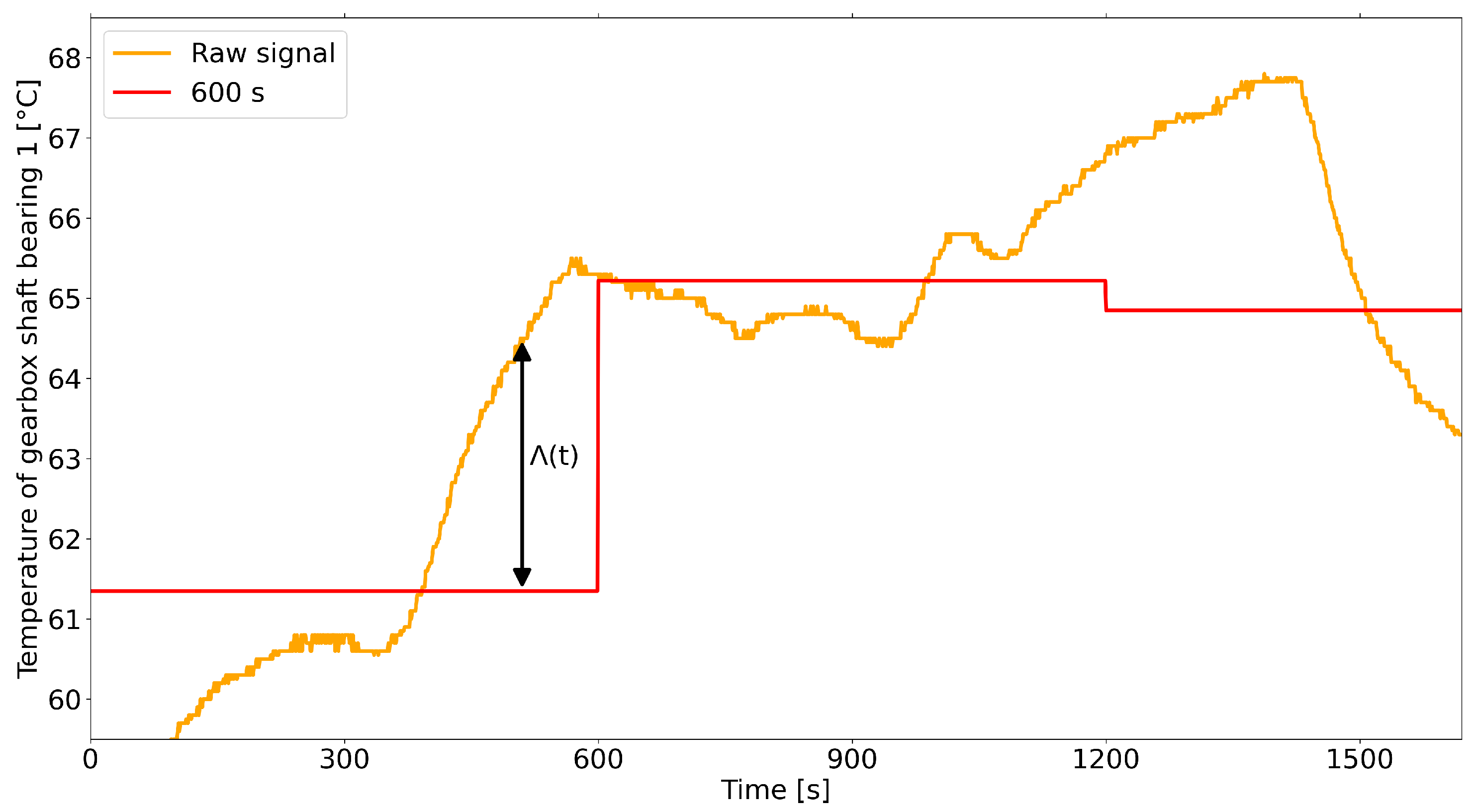
We defined the information loss as the difference between the original signal and its down-sampled signal, i.e., the local error, described by the loss function $\Lambda {\left(t\right)}_{\Delta t_{\mathrm{agg}}}$. The calculation was carried out by further applying the absolute value on the difference, as described in Equation (3):

$$\Lambda {\left(t\right)}_{\Delta t_{\mathrm{agg}}}=|s{\left(t\right)}_{\Delta t_{\mathrm{agg}}}-s{\left(t\right)}_{\Delta t_{\mathrm{org}}}|$$

(3)

In this equation $\Delta t_{\mathrm{org}}$ is the original or native resolution of the data before aggregation. The original signal values are defined as $s{\left(t\right)}_{\Delta t_{\mathrm{org}}}$, the aggregated values as $s{\left(t\right)}_{\Delta t_{\mathrm{agg}}}$ correspondingly. Note that $\Delta t_{\mathrm{org}}=1\mathrm{s}$ for the present dataset. Within a sampling window all values $s{\left(t\right)}_{\Delta t_{\mathrm{agg}}}$ were equal to the averaged raw signal of this window, also known as “value hold”. 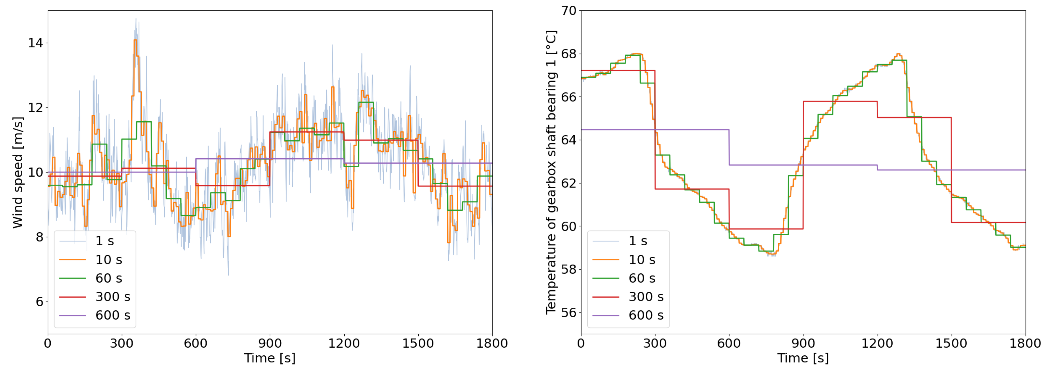Thus, the information loss $\Lambda {\left(t\right)}_{\Delta t_{\mathrm{agg}}}$ always has the same resolution as the original data. A representation of the original and aggregated signal is provided in Figure 4.

Due to the diverse nature of physical quantities measured by the SCADA system, the local errors needed to be normalized to be compared across signals effectively. Normalization also facilitated the interpretation of the results, as it allowed to reason about information losses in relative terms, bypassing the necessity to know the typical operating range of a signal. In our analyses, the interquartile range (IQR) of the values of the raw time series was used as the normalization basis throughout the following parts of the paper if not declared otherwise. The calculated IQR values are listed in

Table 4. List of the available signals and corresponding interquartile range values used to normalize results for comparability. The IQR is defined as the difference between the third and first quartile of a distribution.

Signal Name	IQR	Unit
Active power generation	1052.1	kW
Ambient temperature	6.8	°C
Current phase A	843.0	A
Current phase B	842.0	A
Current phase C	838.2	A
Generator speed	804.5	rpm
Grid frequency	0.098	Hz
Pitch angle blade 1	1.6	deg
Pitch angle blade 2	1.6	deg
Pitch angle blade 3	1.5	deg
Power factor	1.998	-
Rotor speed	7.8	rpm
Temperature inside nacelle	12.0	°C
Temperature of gearbox oil	4.9	°C
Temperature of gearbox shaft bearing 1	6.0	°C
Temperature of gearbox shaft bearing 2	8.2	°C
Temperature of generator bearing 1	11.6	°C
Temperature of generator bearing 2	5.1	°C
Temperature of generator stator	6.0	°C
Temperature of main bearing	5.5	°C
Top box temperature	10.9	°C
Voltage phase A	5.5	V
Voltage phase B	6.4	V
Voltage phase C	6.1	V
Wind direction	151.5	deg
Wind speed	4.4	m/s
Yaw angle	153.4	deg

. We chose this range over other common approaches, e.g., the minimum to maximum distance, to deal with the presence of unavoidable outliers. At the same time the IQR normalization could deal with multi-modal signals that might alternate between two regime states, rarely taking in-between values. Here, working with the the standard deviation could lead to obscure results.

The analysis was performed on a set of 1000 hours of operation, i.e., approximately 0.8% of the entire data set, that was randomly sampled from the complete time series of all wind turbines. For this method the time resolutions varied from 5 to 600 s, the latter being the typical timescale of SCADA data for commercial wind farms.

Results

 

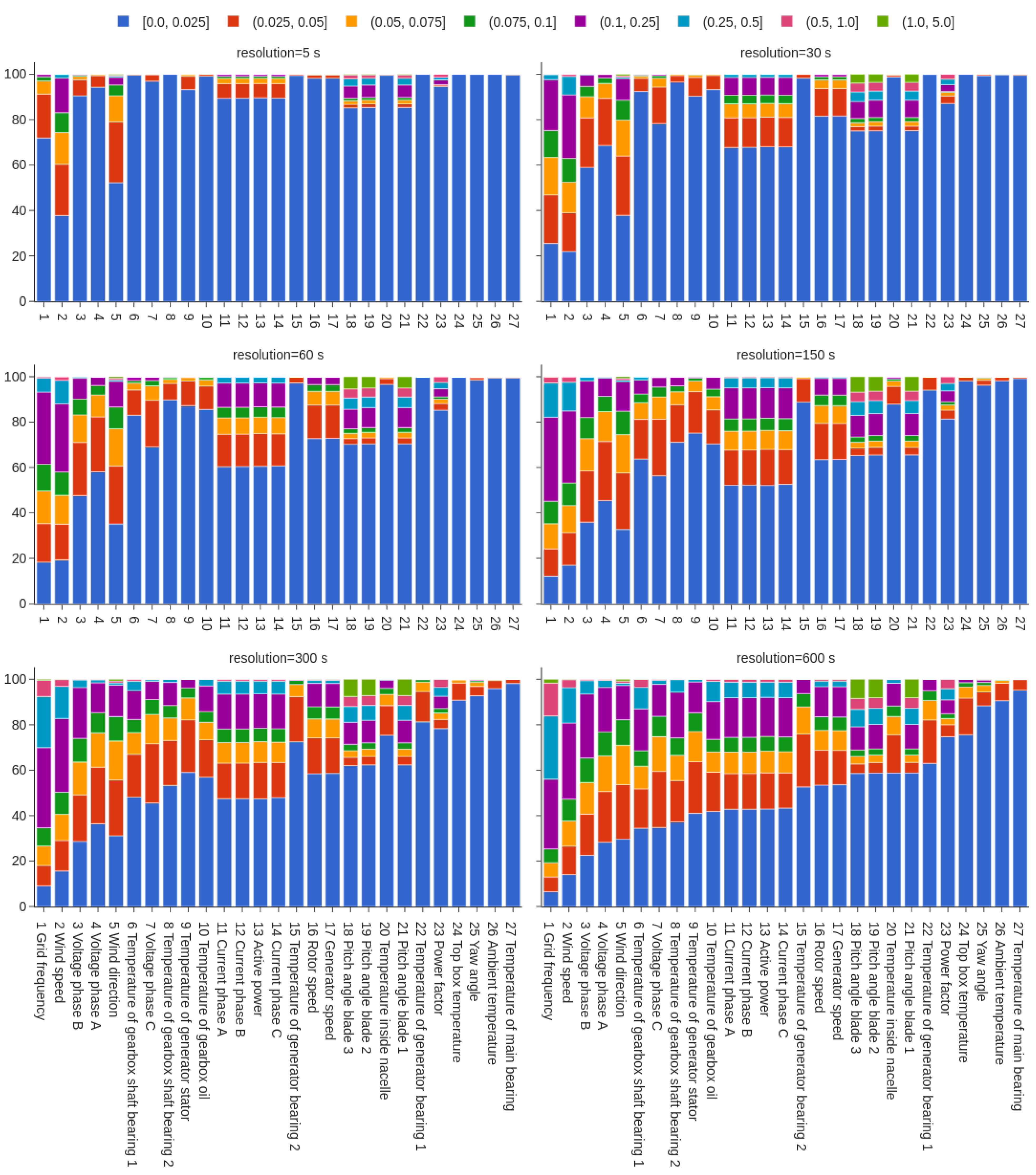
The resulting normalized information loss function values $\Lambda {\left(t\right)}_{\Delta t_{\mathrm{agg}}}$ were grouped into bins of error size. Then, the percentage of data in each bin was calculated, providing us an overview about the severity of the information loss for each signal after an aggregation in various resolutions. In Figure 5 the results are presented: each signal was assigned one bar lined up on the x-axis, colors represent the aforementioned error bins. The margins of these bins are defined as fractions of the normalization basis. The height of each bar is given by the percentage of data in the corresponding error bin. The signals are sorted in ascending order from left to right on the horizontal axis according to the percentage of data in the lowest error bin of $[0,0.025]\times \mathrm{IQR}$ at the largest aggregation period of 600 s. Each signal is assigned a number in the bottom-most axes to allow for better orientation in the upper plots. This representation allowed us to yield an information loss added up from the local error, to compare different signals, and to determine the most affected signals. Moreover, it provided a quantification of the fraction of information that was lost for an assigned resolution for each signal. Tables with the numerical results are provided in the Supplementary Materials.

When inspecting the results displayed in Figure 5, it is possible to obtain behaviors of the signals, such as critical drops of the information content passing from one resolution to another. Additionally, signals that are heavily affected by information loss can be identified. Some key observations are highlighted as follows:

• The information loss severity, i.e., the maximum error occurring, varied greatly between the signals. Certain signals had roughly more than 1% of data with an error greater than 0.5 IQR, mainly environmental, electrical and control variables, such as frequency, currents, power factor, wind speed, and pitch angles. However, for the temperatures of gearbox shaft bearing 1 and the gearbox oil there was also a small amount of error above 0.5 IQR.
• Generally, temperatures were not particularly affected. Only a fraction of information was lost for the largest aggregation period. A noticeable exception was the aforementioned transmission signals, i.e., gearbox shaft bearing 1 and 2 as well as the gearbox oil temperature, which had less than 50% of the data included in the lowest error bin at 600 s aggregation resolution and, therefore, underwent a relatively high loss of information.
• Wind speed and electric signals underwent a drastic loss of information, even at the short aggregation periods (5 to 30 s). Wind speed data in particular featured only 40% of the data in the lowest error bin, i.e., an error ≤$2.5$% IQR.
• Excluding the wind measurements, the pitch angles, electrical characteristics, and generator and rotor speed, information loss was limited to ≈$18\%$ of data with an error of >$0.025\%$ IQR up to an aggregation interval of 60 s. Above this threshold of 60 s resolution, most signals began to lose a considerable amount of information, as the shrinking percentage of data in the lowest error bins indicated.
• Current and active power signals are strongly affected for resolutions above 5 s. Changing the aggregation from 5 s to 30 s causes a loss of >$20\%$ of the total data in the lowest error bin of $[0,0.025]\times \mathrm{IQR}$. While the amount of data in this lowest error bin kept decreasing with a further reduction of the resolution, it was not as drastic as from 5 s to 30 s.
• The typical SCADA data resolution, i.e., 600 s, was not sufficient to correctly represent wind measurements, electrical signals, and the temperatures of gearbox and generator components as more than 20%, even >$50\%$ for the wind speed, of the data have losses greater than 0.1 IQR. On the other hand ambient temperature, main bearing, top box temperature, and yaw angle were barely affected retaining more than 80% of the data in error bins lower than 0.1 IQR
• Pitch angle values were occasionally affected by large differences between the aggregated and original signal. Approximately 10% of the data manifested losses superior to 1 IQR, even at short aggregation periods such as 30 s.
• The transition from 150 to 300 s caused a visible drop from approximately 90 to 70% of the size of the lowest error bin of the generator bearing temperature.

Behavior of Temperature Signals

 

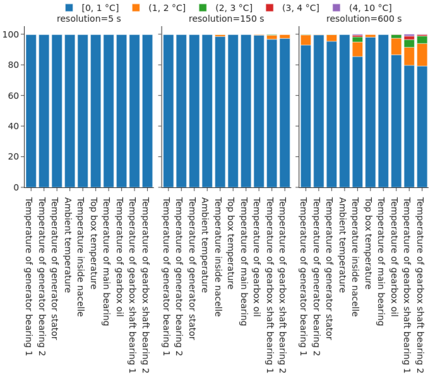
Temperature signals constitute a special interest subgroup, as they are typically used as inputs for predictive maintenance to monitor the status of turbine components. Therefore, we conduct a separate investigation specifically for temperatures. Here, a normalization of results was not necessary as all temperatures already shared the same physical unit, i.e., degrees Celsius.

The results for selected aggregation times are presented in Figure 6. Except for the error bins now in °C, it is the same representation as in the previous part. All data are provided in the Supplementary Materials. The following observations are emphasized:

• Up to an aggregation period of 150 s information losses above 1 °C were almost nonexistent. More than 97% of the data were contained in the [0, 1 °C] error bin. Only gearbox shaft bearings and internal temperatures had a negligible amount of data in the second error bin.
• The typical SCADA resolution, i.e., 600 s, could be problematic for the temperatures of the gearbox shaft bearings, of the gearbox oil, and inside the nacelle, as only 80% of the data had an error below 1 °C.
• Gearbox shaft bearings and gearbox oil temperatures could occasionally exhibit information losses higher than 2 °C and more rarely higher than 3 °C for aggregation periods of 600 s.

Turbine-Dependency

 

The results of the previous calculation of $\Lambda {\left(t\right)}_{\Delta t_{\mathrm{agg}}}$ could also be split between turbines, obtaining a breakdown of the information loss across the whole wind farm, as shown in Figure 7. This analysis allowed us to verify whether information loss was a condition imputable to the behavior of single turbines, or rather a generalized phenomenon affecting all turbines in the farm. Only a selection of temperature signals and resolutions is presented, the complete results table can be found in the Supplementary Materials. The following observations can be drawn:

• Not a single turbine or a set of turbines was responsible for the entire amount of information loss.
• There were variations in the amount of lost information across turbines. For example, observing the percentage of data of the gearbox shaft bearing temperature with an aggregation time of 600 s for which the aggregation error was below 1 ºC, the differences between turbines could vary within a range greater than 20%. In particular turbines WT04 and WT06 had slightly more than 60% of the data in the lowest error bin versus turbine WT02, WT03, and WT11 that had approximately 90% of the data within the 1 ºC error range.
• The differences between turbines were principally only visible for transmission related signals, i.e., gearbox oil and gearbox shaft bearing temperatures. For all other temperatures differences between turbines were not noticeable, as information losses were overall very limited.
• Aggregating the signal at a lower, yet still coarse time resolution, i.e., 300 s, reduced the differences between turbines. The variation range was closer to 10% in this case.
• While shorter aggregation periods reduced the differences between turbines, it did not change the relative impact of information loss within the wind farm. This means that the most affected turbines at 300 s aggregation were also the ones showing greater losses at 600 s.

Seasonality-Dependency

 

Furthermore, the results could be divided into subgroups of the month of the year, as the information loss behavior may vary along the seasons due to environmental conditions such as the wind. Figure 8 shows the variation of information loss for temperature signals throughout the year. Each month was assigned a bar, error bins and aggregation resolutions were set as in previous figures. Results for signals and resolutions not included in the figure are provided in the Supplementary Materials. The results show:

• A seasonal variation in the amount of lost information was visible for gearbox oil and gearbox shaft bearings temperatures. For the 600 s aggregation period, the percentage of data having an error below 1 °C decreased by approximately 10% between summer and winter months.
• The highest losses were registered during the months of November, December, and January when the percentage of data below 1 °C error was around 70% and 80% for the gearbox shaft bearing 1 and gearbox oil temperature respectively.
• It must be pointed out that the temperature of the gearbox oil and of the gearbox shaft bearings had a non-negligible error above 2 °C that slightly increased during the winter months.
• This seasonal dependence was also present for resolutions of 300 s, 150 s and, partly, 60 s. Due to the very low overall error, it was no longer visible for higher resolutions.
• The rest of the temperature signals were much less affected by seasonality and information loss in general. No clear differences between summer and winter months were seen in our analysis.

Discussion

 

Within the scope of our local error approximation, wind measurements and electrical signals are largely affected by a loss of information both at short and long aggregation periods. A certain cause for this behavior is the high variability of these signals. For temperatures, on the other hand, much less error is induced by aggregation. For example, the temperature of the main bearing has more than 90% of the data with an information loss between 0 and 0.025 IQR. Thermal inertia most likely play an important role, such that the data already undergo an intrinsic reduction of the dynamics. Within all investigated temperature signals, the gearbox and generator sensors are noticeable exceptions, as they show a substantial loss of information having less than 50% of the data within the smallest error bins for 10 min aggregation. Figure 5 not only helps to quantify information loss within different signals, but also determines which measurements are most critical and thus require shorter aggregation periods.

The information loss phenomenon is relevant since it affects all turbines, as Figure 7 shows. Some turbines are affected more than others (WT04 and WT06 in the example), but overall all turbines show information loss. Moreover, knowing that some turbines are more affected than the others can be useful for modeling the behavior of the whole wind farm. In fact, these differences could indicate an existence of diverse behaviors within the turbines. However, these strong differences between the turbines within our data might also boil down to our randomly chosen sample size of 1000 h resulting in merely an average of 84 h per turbine.

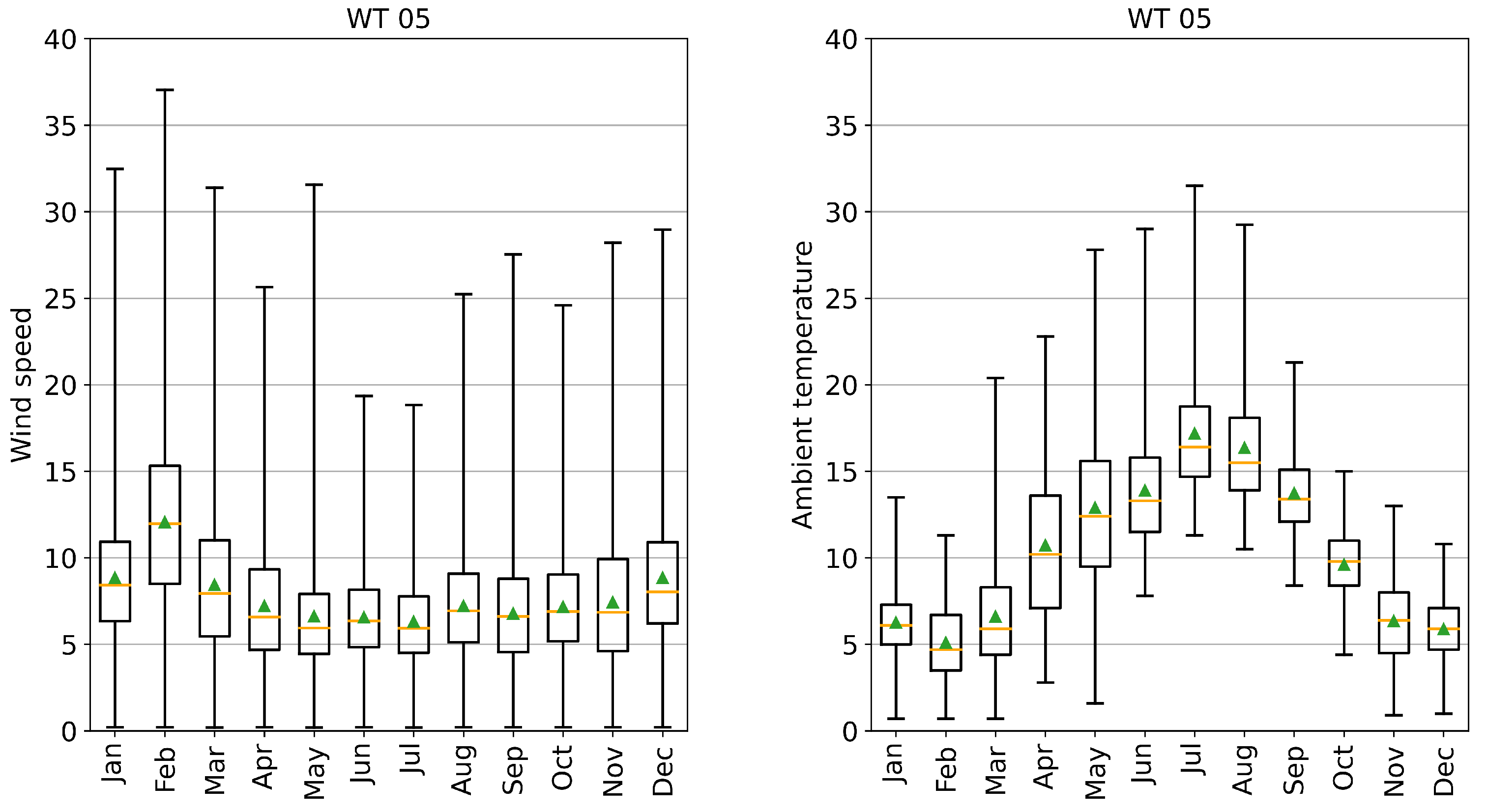
It is further observed that information loss referred to transmission related temperatures is affected by seasonality. Figure 8 shows signs of such effects. For the gearbox oil and gearbox shaft bearing temperatures, an increase of 10% in the data of the [0–1 °C] error bins of the winter months with respect to the summer could be related to the variability of environmental conditions. Lower and stable wind speeds lead to lower variations in operating conditions and, consequently, less dynamics in the form of steep gradients in the temperatures of the gearbox. This results in less differences between the original and aggregated signal. Similarly, differences in external temperatures might increase or decrease the gradients of component temperatures. Figure 9 shows the wind speed and ambient temperature along the year for an exemplary turbine WT05. Note that almost identical profiles are observed for the rest of the farm. As expected, summer months are warmer, but also the range of variation as well as the average value of wind speed is lower when compared to winter. This supports the assumption of an influence of the environmental variability on an increase in information loss.

In conclusion, the choice of the aggregation period for each signal is subjected to a benefit-costs analysis in which the ultimate use of the signal as well as data storage and transmission costs play a contrasting role. However, to detect pre-failure states higher resolution might be needed as anomalies could manifest themselves on shorter timescales. With all these considerations, wind related measurements should be stored at the highest frequency possible since their dynamics is particularly fast and the lost information are useful for any fine-grained analyses that takes the wind behavior into consideration. A similar recommendation can be given for electrical signals that accumulate a visible amount of information losses for resolutions above 60 seconds. Temperature signals are less affected by the phenomenon of information loss upon aggregation. Consequently, they can safely be stored at lower frequencies, even though the standard SCADA resolution of 10 min is not recommendable. Concluding from the investigations, at least 150 to 300 seconds should be preferred.

4.2. Q2: Do External Conditions Have an Effect on Information Loss?

Knowing that operating conditions of turbines vary considerably both on short, i.e., hours, and long timescales, i.e., months of the year, an analysis of the relation between information loss and external conditions is presented. As wind speed is one of the most important parameters governing turbine operations, the analysis focuses specifically on this.

The objective is to characterize the behavior of the information loss with respect to the wind speed. We answer the questions whether certain wind conditions cause larger deviations in the aggregated signal and, if so, what the expected range of information loss is. Then, the behavior of different signals is compared to analyze possible shared patterns—such as certain wind speed regions—for which most signals show large variations in information loss.

Methodology

 

To capture the influence of wind conditions, the information loss results were divided into bins of wind speed with a size of 0.5 m/s. This value is commonly used to group data for power curve calculations and analyses of the turbine behavior [42].

Two complementary perspectives on the problem were proposed. The first attempts to capture the overall behavior of the available signals, with the objective to determine shared trends. This was accomplished by sorting the results of Equation (3) by wind speed. For each bin the mean value of information loss was computed. Like throughout the rest of the paper the IQR was used as the normalization basis. The second perspective is a detailed representation of the span of information loss per wind speed bin for each individual signal, providing an estimation of the range of variation. The range defined by the 5-95^th percentile of the distribution was calculated for the different signals and for each wind speed bin. For this analysis the sign of the deviations from the original signal is relevant and must be preserved. Thus, Equation (3) was modified to Equation (4), where the direction of the difference between aggregated and raw signal is no longer omitted, resulting in a newly defined signed information loss:

$${\Lambda }^{\pm }{\left(t\right)}_{\Delta t_{\mathrm{agg}}}=s{\left(t\right)}_{\Delta t_{\mathrm{agg}}}-s{\left(t\right)}_{\Delta t_{\mathrm{org}}}$$

(4)

Results

 

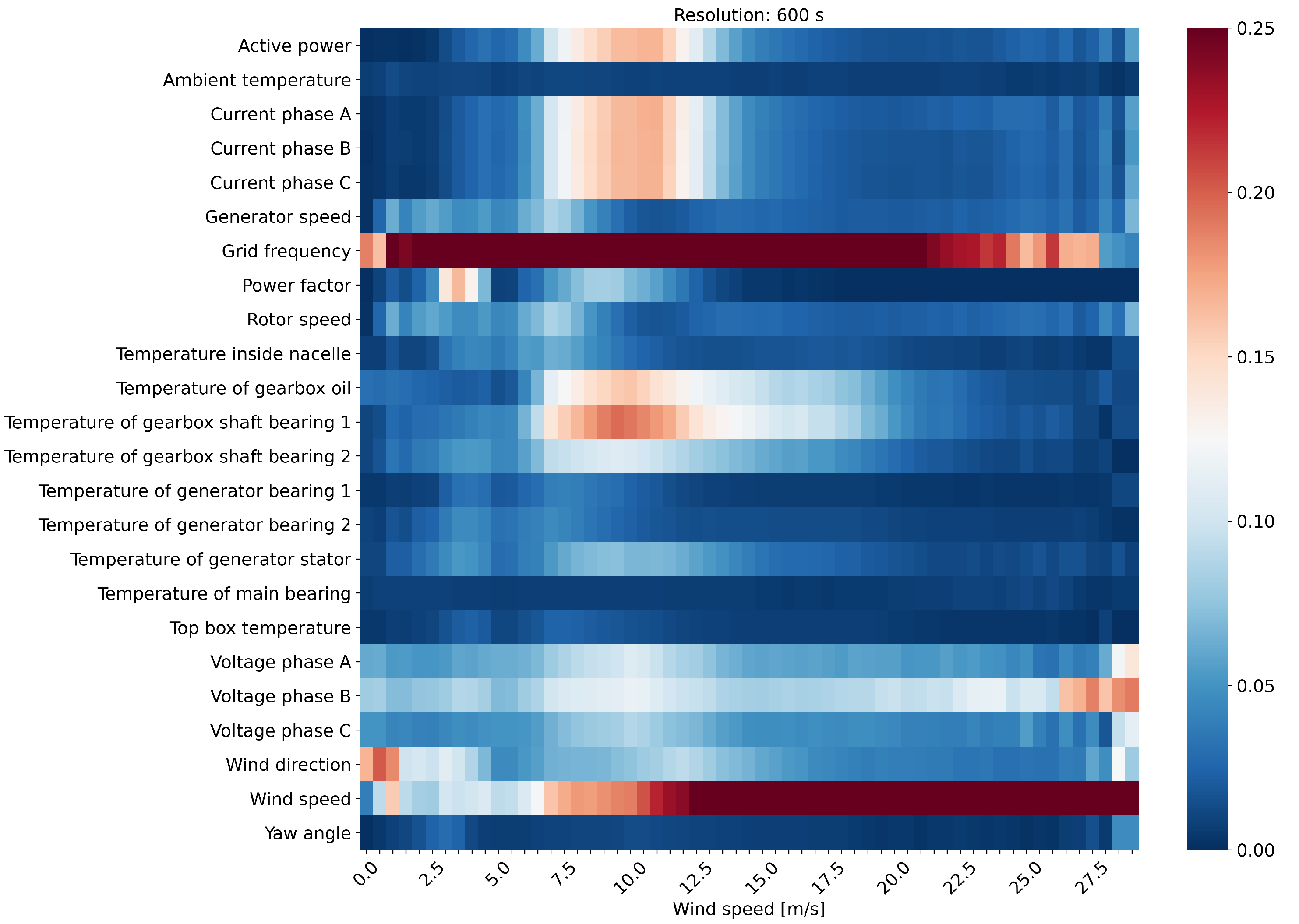
The normalized results of the mean information loss for each signal are represented in Figure 10 in the form of a heat map, such that signals can be easily compared to each other. The horizontal axis shows wind bins with a width of 0.5 m/s, the vertical axis lists the signals. The magnitude of the mean information loss for a given condition is determined by the color of the cell. Notice that the color scale is capped to a value of 0.25. Otherwise, i.e., with a full scale, the grid frequency and wind speed error values would completely mask variations in the rest of the signals. Additionally, the signals of the pitch angles are not included as they show a very large variation, augmented by the low value of their IQR. For analyzing the behavior of these signals please refer to Figure 11. Results for all temporal resolutions are available in the Supplementary Materials.

From an overall perspective it can be noticed that active power, all currents, gearbox oil, and gearbox shaft bearing temperatures were characterized by a quite large mean information loss of 0.12 to 0.2 IQR for wind speeds ranging from 7 to 12 m/s. This range corresponds to the upper part load region of the power curve. Other signals follow that trend but had less pronounced maxima here such as the power factor, the temperature of the generator stator and the voltages. Albeit, the voltages showed another maximum for high wind speeds around 25 m/s. Another group of signals with the rotor and generator speed as well as the temperature within the nacelle were characterized by overall lower average losses and their maxima were located around wind speeds between 5 and 7 m/s just above the typical cut-in wind speeds of wind turbines. The frequency value had the maximum error outside the range of our heat map. However, its red band shows us that most information was lost in the operating region of the turbine from 2.5 up to 20 m/s. The wind speed itself had most of its information lost for high wind speeds. The remaining signals had a much lower span of variation of their information content. Therefore, no critical wind regimes could be easily identified. Overall, Figure 10 clearly shows that there were shared patterns in information loss between signals, but these were not unique. Some signals had larger information losses during the transition toward nominal power conditions, others were more affected at lower wind speeds, others again for high wind speeds, and finally certain signals were barely affected by changes in the range of information loss.

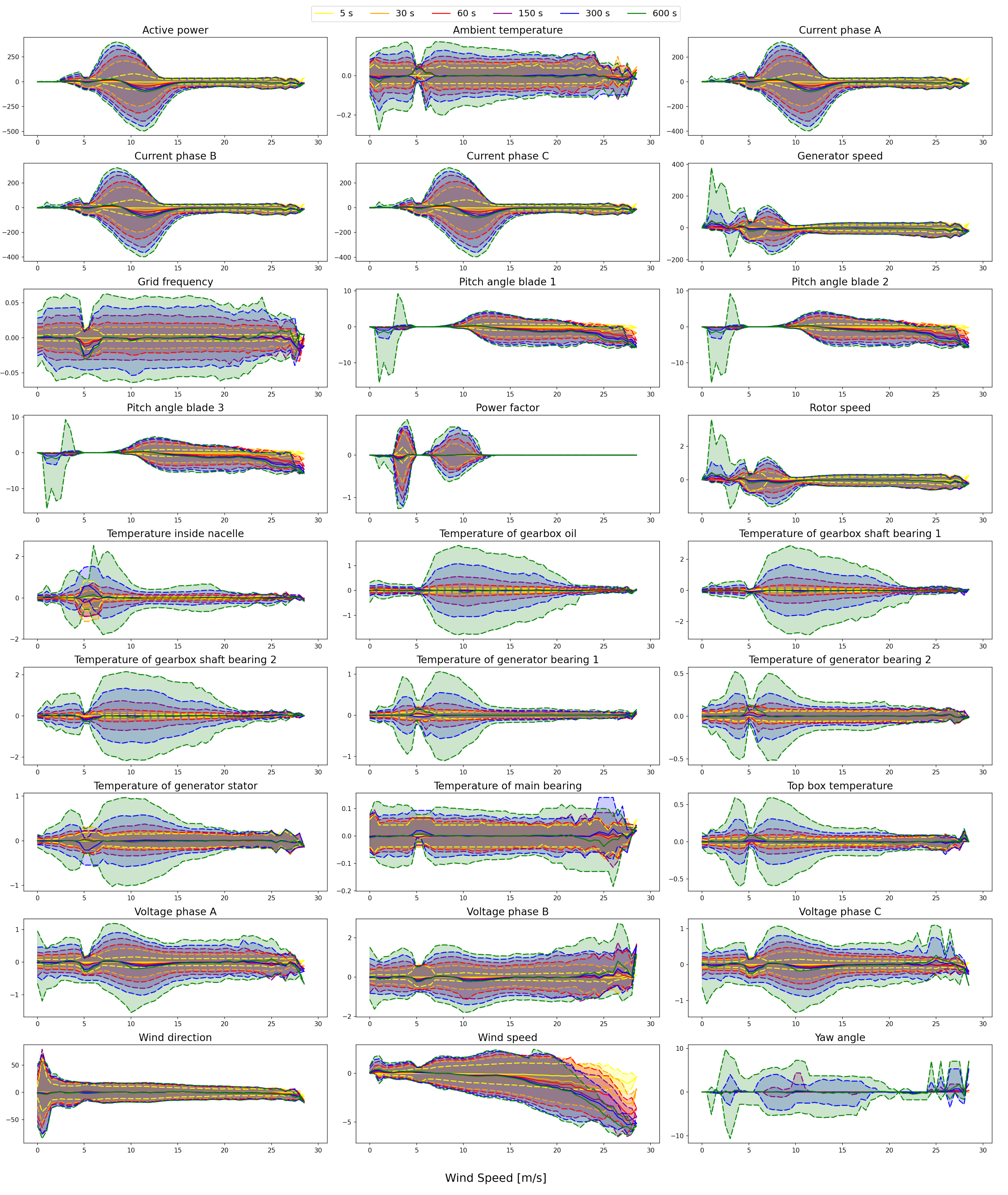
A second perspective focuses on the quantification of the the expected range of variation of information loss. Thus, the 5–95th percentile of the distribution of the signed local error and the mean value were sorted into the same wind bins of 0.5 m/s already used above for different levels of signal aggregation. The results for all available signals are represented in Figure 11. Values of information loss are reported in the native units of the signals without any normalization, allowing for an easy interpretation of the results. The plots further allowed us to visualize the typical profile of information loss with respect to the wind speed. Additionally, it was possible to quantify the extreme range of variation of the information content that can incur as a consequence of aggregating signals. Figure 11 is organized into subplots in which each individual signal has its own subfigure. The wind speed is assigned to the x-axis measured in m/s, on the y-axis the values of the signals in their original units are reported. Positive values indicate that the aggregated value is above the raw data, negative values the inverse, respectively. The dashed lines correspond to the values of the 5–95th percentile for each aggregation level in different colors.

The first observation to Figure 11 is that range of the variations in information loss always increased with the aggregation time. Some signals, in particular grid frequency, ambient, and main bearing temperature, showed little variation over the entire range of wind speed values, the span of the 5–95th range was almost constant for all wind conditions. All other signals had visible variations in their information loss ranges and their mean values oscillated around zero. As it can be seen from the dashed lines, there were some instances for which the difference range between the original and aggregated signal was particularly large, even pronounced peaks could be obtained: Those peaks can either be symmetric around 0, e.g., for all temperatures, or asymmetric, as was the case for the active power, the pitch angles, the currents, and also slightly for the voltages.

The error range was prominently large for the active power for wind speeds between 6 and 12 m/s and aggregations of 300 to 600 s with an information loss between −400 kW and 400 kW. Currents also varied heavily in that wind speed region with an information loss span between −400 and 300 A. Additionally, in the same region, temperatures had their maximal variations, in the case of the gearbox shaft bearings as high as −3 to 3 °C. However, little to no variation is seen for the main bearing temperature whose range of variation is between −0.20 and 0.35 °C. For signals such as rotor, generator speed, and the temperature of the generator bearing the range of variation of information loss was high for lower wind speeds. It was greatly reduced and constant once at nominal operating conditions with wind speed above 12 m/s. The highest error range could be observed for very low wind speeds below 5 m/s. Additionally, for pitch angles the error is extremely high with −15 to 10 deg for these low wind speeds. A similar trend of an almost constant error range for wind speeds above 12 m/s could be seen in most of the temperatures. Though, especially for temperatures related to the gearbox the transition to this constant regime was much smoother and the span of the range approached low values only for very high wind speeds, i.e., winds above 20 m/s. While most signals showed large variations around the transition phase towards nominal power, a noticeable exception was the wind direction that varies greatly between −75 and 75 degrees for wind speeds around 0 m/s and stabilized between −25 and 25 degrees for wind speeds above 5 m/s. A further prominent observation was the error of the pitch angles for wind speeds between 5 and 10 m/s where it stayed almost at 0.

The error of the wind speed itself increased steadily with increasing wind speed. Furthermore, the mean value of the error decreased, meaning an underestimation of the wind speed upon aggregation.

As a general additional remark: For aggregations up to 60 s the variation of information was low compared to aggregations of 300 to 600 s. As an example, in the case of the gearbox shaft bearing 1 temperature, information loss spanned well below −1 and 1 °C for aggregations up to 60 s, whereas for 600 s aggregation this range varied between −3 and 3 °C.

Discussion

 

The two analyses show that for the wind speed dependence of the information loss there is no shared pattern between all investigated signals. Nevertheless, we identified regions where maxima of the error due to aggregation can be located within the signals investigated: Below the operational regime, i.e., <5 m/s, in the transition state of the turbine from around 6 m/s to 12 m/s, and in the cut-off region above 25 m/s.

In the first region, the turbine is typically either in idle state, turned off, just starting up, or right after shutting down. The error in the generator and rotor speed most likely is caused by this start-up/shut-down transition. The asymmetry of the error in Figure 11 supports this assumption as the error for lower values of <3 m/s is positive, i.e., the aggregation value is higher than the raw value. This behavior is the consequence of the rotational speed going down. In this particular case, also the pitch angle might be part of the transition to an idle state as the asymmetric behavior is the same with the opposite sign. The complete shutdown sequence might, however, contain important information about the health of the system that is lost by aggregation.

The second region, corresponding to the part load region of the power curve is critical for various signals. As this is a transition phase from idle condition to the full power regime, the turbine behavior is highly dynamic, leading to short term variations in the operational data. Therefore, aggregated and original signals diverge considerably. The asymmetry of roughly 5 m/s in the error span and the mean of the active power, currents, and also voltages in Figure 11 shows a general overestimation of the raw data values around 7 m/s and an underestimation for higher values around 12 m/s.

In contrast, for signals like main bearing, top box, and ambient temperature as well as the yaw angle there are no regions with large information losses. The range of variation is almost constant along the whole wind speed range. The span curves of Figure 11 might be misleading here: The error ranges are mainly below 1 °C. For a control parameter like the yaw angle this might be due to the fact that it is not directly connected to any operational state. Nevertheless, it is quite surprising that even some temperature signals of bearings do not exhibit a maximum in this dynamic transition region. One reason is most probably the thermal inertia of the material, especially for large bearings.

There is a further group of signals with the voltages that have a higher information loss also for very high wind speeds, i.e., above 25 m/s. Here, the cut-out process of the turbines could be the main influence. In the same region also the yaw angle has an error maximum. Information about the cut-out process will, therefore, be lost, when aggregating the data in low resolutions. Again other signals, such as wind direction, rotor and generator speed, and the temperature inside the nacelle have their highest errors for low wind speeds, i.e., below 5 m/s. In this region the wind direction changes more often. The errors in the generator and rotor speed most likely result from the turbine turning up or down. However, this might contain important information about the health of the system. The wind speed itself carries increased error with increasing wind speed. Its simultaneous increase in underestimation by aggregation is most likely caused by sudden bursts of wind that barely contribute to an aggregated mean value.

These observations provide useful insights on the behavior of turbine signals under specific wind conditions. In particular, they show that the accuracy of aggregated measurements is not independent from wind conditions. Gearbox behavior, for example, can vary visibly within the part load region of the power curve. Higher frequency of the data would be more appropriate to monitor and characterize these operating conditions. Figure 11 complements the analysis providing a quantification of the information loss for the different signals at various time resolutions.

The two complementary perspectives allowed to determine critical conditions during turbine operations. Various signals show a large fraction of the aggregation error concentrated for the part load and upper part load regions of the power curve. Moreover, while the aggregation error might be negligible for some signals, such as the main bearing and ambient temperature, for others, in particular active power, currents, and gearbox related temperatures, this error must not be ignored. Decreasing the length of the aggregation period to a value between 60 to 150 s greatly helps reducing the maximum extent of information loss range, maintaining a limited discrepancy between aggregated and raw signal. Moreover, knowing the link between wind speed and error provides relevant knowledge for improving the design of models aiming to describe turbine behavior.

4.3. Q3: What Is the Recommended Aggregation Frequency?

To find the optimal trade-off between minimizing the data footprint and preserving enough information to model and assess the turbine behavior, it is necessary to study the relation between information content and aggregation frequency. By knowing the behavior of an information loss over resolution it is possible to determine the critical aggregation time for a given signal, after which a great part of the information is inevitably lost. Thus, these information can be used to chose a suitable data storage solution.

Methodology

 

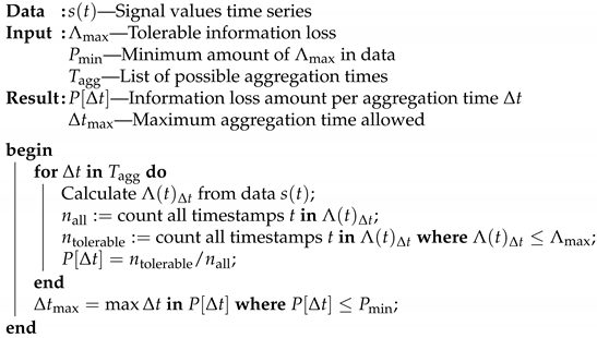
To address this relevant question the following methodology was used, that is also summarized in Algorithm 1.

Algorithm 1: Determination of the maximum aggregation time allowed for a prechosen tolerable information loss of a signal.

First, a maximum tolerable error ${\Lambda }_{\max }$ and a minimum amount of data points $P_{\min }$ with an error lower than this error was defined. As we wanted to compare our results to each other, we used IQR normalized signal values. Therefore, ${\Lambda }_{\max }$ must be given in a percentage of the IQR. Of course, if only one signal was investigated this tolerable information loss could also be defined in real units.

Then, for each signal $s\left(t\right)$ and resolution $\Delta t$ out of a list of possible aggregation resolutions $T_{\mathrm{agg}}$, the information loss $\Lambda {\left(t\right)}_{\Delta t}$ was calculated as defined in Equation (3). This allowed us to determine the percentage $P[\Delta t]$ of data having an aggregation error lower than the chosen threshold. Thereafter, the maximum aggregation time $\Delta t_{\max }$ could be derived by finding the highest resolution possible for $P[\Delta t]\le P_{\min }$. Of course, the choice of the maximum error threshold had to take into consideration the final use of the data as well as the marginal cost of storing additional information.

Results

 

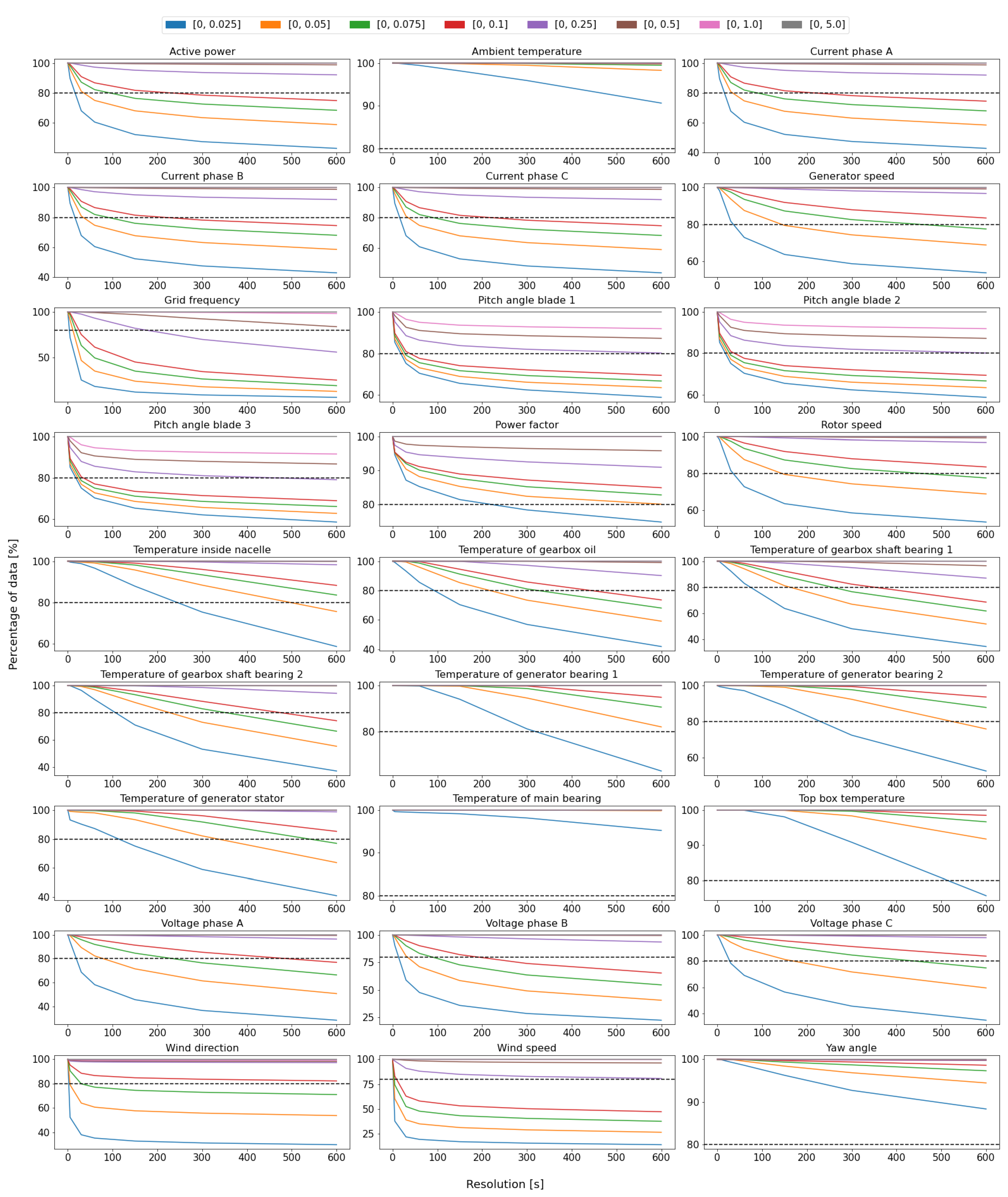
For Figure 12 we chose various tolerable error thresholds that define our closed error-bins $[0,{\Lambda }_{\max }]$, see legend, and analyzed the available signals for a resolution range varying from 0 to 600 seconds. The horizontal axis shows the time resolution in seconds. On the vertical axis the percentage $P[\Delta t]$ of data having an aggregation error lower than the error threshold is represented. We further chose a reasonable minimal amount of $P_{\min }=80\%$ for further evaluation of the curves, indicated by a dashed line. As the figures do not share the same scale on the y-axis, it also facilitates a better orientation. Numerical results are available in the Supplementary Materials. The resulting curves show the information loss amount over resolution and lead to the following observations:

• There existed different behaviors depending on the nature of the signals. Some signals followed an “elbow curve” trend, whereas others—these include mainly temperatures—showed a more linear decay or no decay at all in information loss.
• The steepest drops were associated with wind speed and its direction, such that even short aggregation periods had less than 50% of the data below the 0.1 and 0.025 IQR error threshold respectively. Electrical signals, grid frequency in particular, also had clear drops in accordance with the results obtained in Section 4.1.3.
• Within the temperature signals, the ones related to the gearbox showed significant information losses at 600 s resolution. More than 25 to 30% of the data were above the 0.1 IQR error threshold.
• The inflexion point, i.e., the point of the strongest change in the slope, of the elbow curves indicates the aggregation period above which most of the information in the signal was lost. It can be seen that for most signals this inflexion point, for this specific error threshold, lay between 100 and 200 s.
• The higher the tolerable error was, the longer the optimal aggregation periods size could be, as the inflexion point moved towards larger values. This was explicitly shown by the rotor speed and grid frequency signals.

Discussion

 

Figure 12 is a proposed method for choosing the ideal resolution for turbine signals. It allows to determine the optimal resolution of a signal with the definition of a maximum error ${\Lambda }_{\max }$ and the minimum percentage $P_{\min }$ of data that should not exceed this limit. The inflexion point that is visible for most curves determines the aggregation period, above which most of the information and details of the dynamic of the signals are lost. This allows to determine a sweet spot for SCADA data storage, allowing to reduce memory footprint of the data without excessive compromises on data quality.

Moreover, the comparison of the profiles of the various curves allows to determine differences in signal dynamics. Signals with inflexion points at low aggregation periods are characterized by faster dynamics. Wind speed, wind direction, and grid frequency have a drop for aggregation periods below 10 to 100 s, after which the rate of information loss with respect to the length of the aggregation period remains almost constant and greatly reduced. Accordingly, most short-term information is contained on very short timescales. Voltage and current measurements have their inflexion point at lower resolutions between 100 and 300 s, depending on the threshold set for the maximum tolerable aggregation error. Other signals, namely temperatures have a different behavior. Instead of elbow curves they show a more linear decay or even no decay at all such as for the main bearing, whose percentage of data below the lowest error threshold, i.e., [0,0.025 IQR] is not lower than 95% even for a 600 s aggregation period.

The choice of the acceptable error ${\Lambda }_{\max }$ and the percentage $P_{\min }$ are highly dependent on the usage of the data as well as the economics of collecting, storing, and processing high volumes of data. Choosing a more restrictive error threshold moves the inflexion point towards lower values of the aggregation period size, but increases the amount of memory necessary to store information. Nevertheless, the proposed methodology allows to take informed decisions on the strategy to store and aggregate SCADA operating data. Moreover, insights concerning the dynamics of the different signals can be inferred by studying the profiles of the signal curves.

5. Summary and Conclusions

This study has aimed to explore the information contained in high frequency SCADA data to determine characteristics and limitations of wind turbine SCADA data. The main goal of this contribution has been to quantify the information lost due to temporal aggregation of operating data, as this data is usually only available as 10-min averaged values.

Simple methods such as the calculation of a set of descriptive statistics and the Kolmogorov–Smirnov test of the original and aggregated signal haven been carried out. Both methods, though, do not provide a clear picture of information loss. Although they show resolution-critical signals, they fail to provide any quantification of the effect of signal aggregation or indications that help to choose the optimal resolution for the signal.

To address this limitations a framework for information loss study has been elaborated. The results of this method highlight wind data and electric signals as heavily affected by information loss with less than 50% of the data with error below 2.5% of the interquartile range of the data. Temperature signals are generally less sensitive to aggregation, with the noticeable exceptions of the temperatures of the gearbox that show similar losses to the electrical signals. The presented framework allows to rank and determine the expected information for each signal and a certain aggregation period. A study of seasonal behavior has revealed that for signals measured at the gearbox, i.e., gearbox oil and gearbox shaft bearing temperatures, the information loss only varies approximately 10% between summer and winter months. Information loss is a phenomenon that affects all turbines of the analyzed wind farm, but variations in the aggregation error are seen between turbines.

Besides these approaches that pool together the whole operating regime, also the effect of wind speed on information loss has been investigated. Our study reveals that for various signals, temperatures in particular, ramping up from a stopping to rated power state causes the largest variations in the extent of information loss. Variations of an error in a 10 min aggregation interval of up to 400 kW for the active power, up to 400 A for the currents, and up to 3 °C for the main bearing temperature are the most noticeable examples of this investigation.

In addition to these considerations, a methodology to choose the optimal signal resolution is provided. To comply with stricter conditions in terms of maximum acceptable error the period of aggregation of the signal should be reduced, requiring larger resources to handle and store the signal.

In conclusion, this research delves into the limitations of typical 10-min SCADA operating data, investigates the effect of data aggregation and provides methods to determine the amount of information that is lost. Wind and electrical signals, and to a less extent temperatures of the gearbox are heavily affected by information loss and should, therefore, be stored at high resolutions of 1 to 5 s. The typical SCADA data resolution of 10 min is not sufficient to capture the dynamic behavior of these signals. The differences between the original and aggregated signal could negatively impact the performance of predictive algorithms and models describing normal turbine behaviors. Knowing the limitations of SCADA is also useful to explain the shortcomings of turbine models. Smarter SCADA data aggregation policies should be considered taking into account the issue of information losses on the various signals.

Future works on this topic can attempt to quantify information loss in terms of local minima or maxima that are lost due to aggregation. This would give further insight into information loss on the signal dynamics. An approach might be the application of Fourier transform to the data to study changes in its dynamics. However, fast changing signals, in particular wind speed, might vary too randomly, eventually making it very difficult to isolate meaningful frequencies. Still, careful filtering during analysis could lead to beneficial discoveries. For further investigations on the effects of external conditions, apart from the wind speed, it might also be important to look at other influences such as the extent of information loss under wake effects, i.e., turbulent conditions. Moreover, the case-study nature of this research does not allow to extend our conclusions to the entire universe of wind turbines, as the effect of geographical position of the wind farm, different turbine manufacturer, and technology could not be addressed.

Apart from these theoretical outlooks, it will additionally be necessary to quantify the impact of an information loss to actual analyses working with aggregated data. Although an aggregated signal might have 95% of its data with a very low information loss, the interesting operating state of a turbine could be hidden within the remaining 5% and might, therefore, be irreversibly lost. Consequently, regarding, e.g., early fault detection, a focus should be set on the question if and how early a failure is detectable with a certain resolution.