Domain Adaptation Network with Double Adversarial Mechanism for Intelligent Fault Diagnosis

Abstract

Due to the mechanical equipment working under variable speed and load for a long time, the distribution of samples is different (domain shift). The general intelligent fault diagnosis method has a good diagnostic effect only on samples with the same sample distribution, but cannot correctly predict the faults of samples with domain shift in a real situation. To settle this problem, a new intelligent fault diagnosis method, domain adaptation network with double adversarial mechanism (DAN-DAM), is proposed. The DAN-DAM model is mainly composed of a feature extractor, two label classifiers and a domain discriminator. The feature extractor and the two label classifiers form the first adversarial mechanism to achieve class-level alignment. Moreover, the discrepancy between the two classifiers is measured by Wasserstein distance. Meanwhile, the feature extractor and the domain discriminator form the second adversarial mechanism to realize domain-level alignment. In addition, maximum mean discrepancy (MMD) is used to reduce the distance between the extracted features of two domains. The DAN-DAM model is verified by multiple transfer experiments on some datasets. According to the transfer experiment results, the DAN-DAM model has a good diagnosis effect for the domain shift samples. Moreover, the diagnostic accuracy is generally higher than other mainstream diagnostic methods.

1. Introduction

In the process of operation, rotating machinery equipment is often subjected to sudden load increase and load reduction, resulting in stress and speed change of rotating machinery equipment [1]. These sudden load changes and sudden speed changes easily cause damage to key rotating parts. If they are not found and handled in time, the overall mechanical performance is directly and seriously affected and certain economic losses and even casualties may be caused [2,3,4]. Hence, without affecting the normal operation of mechanical equipment, in the early stage of failure, accurate detection and diagnosis of its health condition is of great significance [5,6].

Over the years, a large number of advanced fault diagnosis methods, such as signal processing [7] and machine learning [8,9], have been proposed successively, which have achieved good results in the field of mechanical fault diagnosis [10,11,12]. However, the above methods more or less rely on expert knowledge and waste of manpower and intelligence is poor. In recent years, the rapid development of deep learning has injected new vitality into fault diagnosis and achieved impressive results. For example, Cheng et al. [13] proposed an intelligent fault diagnosis method for rotating machinery based on local binary convolutional neural networks. Zhao et al. [14] presented an intelligent fault diagnosis method for rotating machinery with local and non-local information based on a semi-supervised deep sparse auto-encoder (SSDSAE). Cheng et al. [15] constructed a novel fault diagnosis method using deep variant sparse filter networks (DVSFN). Gai et al. [16] proposed an internal parameter optimized deep belief network (DBN) method based on the grasshopper optimization algorithm (GOA). Jiang et al. [17] introduced an intelligent fault diagnosis method based on a one-dimensional convolutional neural network (1D-CNN), aiming at the problem of a small number of fault samples. Kolar et al. [18] presented a convolutional neural network-based data-driven intelligent fault diagnosis technique for rotary machinery which uses a model with optimized hyper-parameters and network structure.

Although deep learning has made remarkable achievements in the field of fault diagnosis, careful study shows that these methods are all based on the premise that training data and test data belong to the same distribution. However, this situation does not exist in a real state in which the sample distribution of training data is different from that of test data. Thus, the trained model (the distribution of training data and test data is the same) is not suitable under this condition and the diagnosis effect is poor or even invalid. Therefore, for the sake of solving the problem of inconsistent data distribution, the domain adaptation [19] comes into being. The general frame diagram is shown in Figure 1.

As the most commonly used transfer learning method at present, domain adaptation does not require that training data and test data have the same distribution. This method successfully solves the dilemma faced by the current mechanical fault diagnosis field [20]. However, complex problems cannot be solved effectively only by relying on the domain adaptation model, which is due to the model established on the basis of a shallow learning model, so as to limit learning ability. With the rapid development of deep learning, more and more researchers combine domain adaptation with deep learning to study the theory of deep domain adaptation learning and establish the diagnosis model of deep domain adaptation.

Lu et al. [21] developed a new deep neural network model with domain adaptation for fault diagnosis. Li et al. [22] introduced a method that extracts machine-invariant features using a deep auto-encoder and aligns the extracted features using domain adaptation to achieve cross-machine fault diagnosis. Singh et al. [23] raised a novel domain adaptation method based on deep learning. Moreover, it achieved good performance for gearbox fault diagnosis under velocity changes. Xu et al. [24] came up with a neural network named discrete-peak joint attention enhancement (DPJAE) convolutional model for unbalanced variable speed fault diagnosis. Lee et al. [25] proposed a multi-objective instance weighting-based transfer learning network to solve the problem that the discrepancy between and within domains is large and successfully applied it to fault diagnosis. The deep domain adaptation model can get rid of the inherent disadvantages of the domain adaptation network with the help of a deep learning network and also maintain the advantages of the domain adaptation model, which can effectively solve the problem of data sample distribution discrepancy [26].

In recent years, a large number of researchers is focusing on adversarial learning represented by generative adversarial nets (GANs) [27]. Various deformation networks based on GANs appear one after another and have achieved good diagnosis effects [28,29,30,31]. Compared with the traditional deep neural network, adversarial learning networks have a great improvement in diagnosis; so, the idea of adversarial learning networks being appended in deep domain adaptation networks is also a hot topic. At present, some remarkable achievements have been attained based on the deep adversarial domain adaptation model. Saito et al. [32] proposed an unsupervised domain adaptation based on maximum classifier discrepancy. Wu et al. [33] introduced a deep transfer maximum classifier discrepancy method that, combined with a batch normalized long-short term memory (BNLSTM) model, successfully solved the problem under few labeled data. Li et al. [34] constructed an adversarial domain adaptation model by adding a domain discriminator and used deep coral to align target domain features with source domain features. Multi-group transfer experiments proved that this model achieved good diagnostic results. Guo et al. [35] presented a deep convolutional transfer learning network (DCTLN), which contained two modules, condition recognition and domain adaptation. The two parts were promoted against each other, thus improving the diagnostic performance of the model to a certain extent.

However, the above approach is considered from a single point of view, with only domain-level alignment or class-level alignment. Only domain-level alignment ignores the task-specific decision boundary and only aligns the characteristics of the two domains completely, ignoring the characteristics of each domain. On the contrary, only considering class-level alignment takes into account the characteristics of each domain, but may be limited by mismatched categories because it does not take advantage of global local knowledge. Consequently, this paper proposes a new fault method, namely, domain adaptation network with double adversarial mechanism (DAN-DAM). This method takes both domain-level alignment and class-level alignment into account and achieves satisfactory diagnostic results.

Figure 2 roughly shows a classification effect comparison between the double adversarial domain adaptation method and other domain adaptation methods. The DAN-DAM model integrates domain discriminator and double label classifiers and uses a deep convolutional neural network (CNN) as feature extractor for feature extraction and the combination of pairs of them forms double antagonism. Specifically speaking, on the one hand, the feature extractor forms an adversarial mechanism with the two label classifiers to realize class-level alignment and Wasserstein distance [36] is used to measure the difference between the two classifiers. On the other hand, the feature extractor and the domain discriminator form another adversarial mechanism to realize the domain-level alignment and the gradient reversal layer (GRL) [37] is used to reverse the gradient automatically. In addition, in the feature extraction stage, maximum mean discrepancy (MMD) [38] is used to reduce the distance between the extracted features of two domains, which avoids the degenerate learning caused by adversarial, so as to improve the accuracy of model diagnosis to a certain extent.

The main contributions of this paper are as follows:

(1)

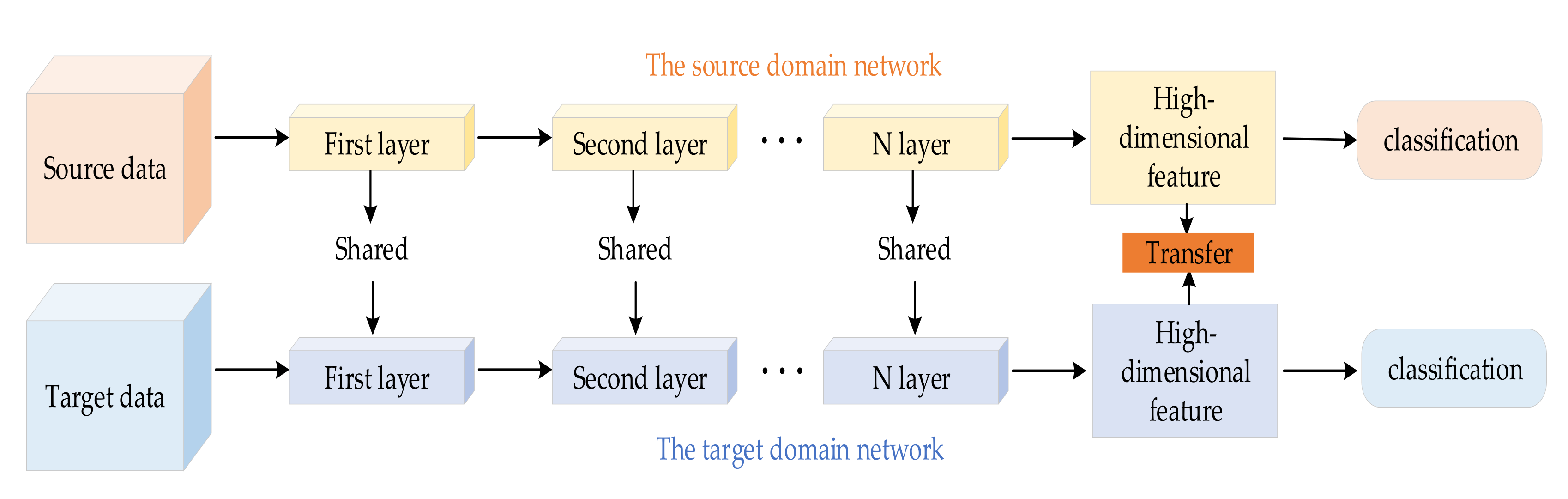
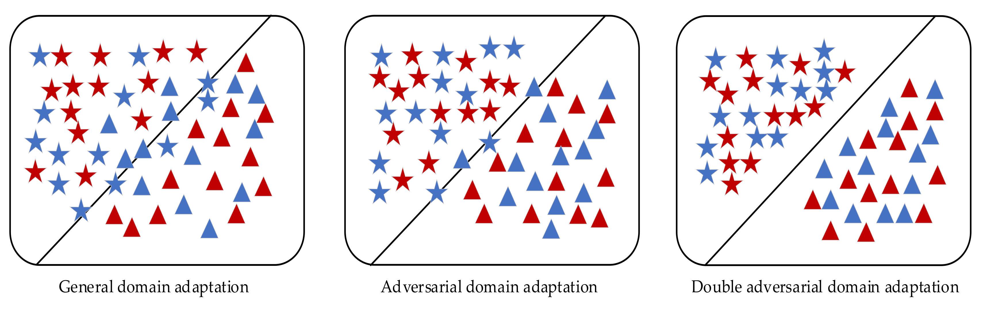
In this paper, a new fault diagnosis method is proposed, which adopts a double adversarial mechanism to realize domain-level alignment and class-level alignment at the same time.

(2)

The proposed method is a novel domain adaptation method to solve the problem that distribution of training data and test data is not the same in a real state. Therefore, the unlabeled target domain samples are the same as the labeled source domain samples, which can be correctly distinguished.

(3)

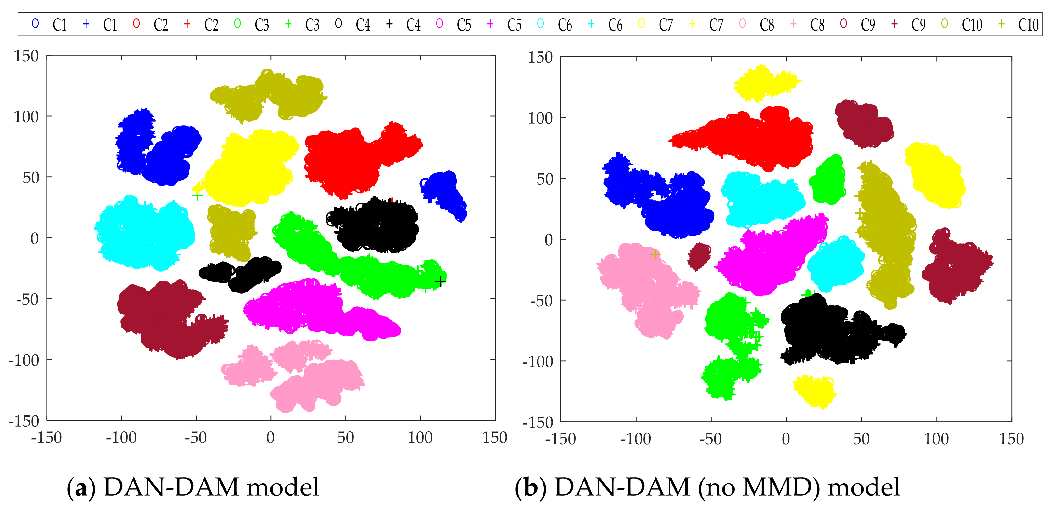
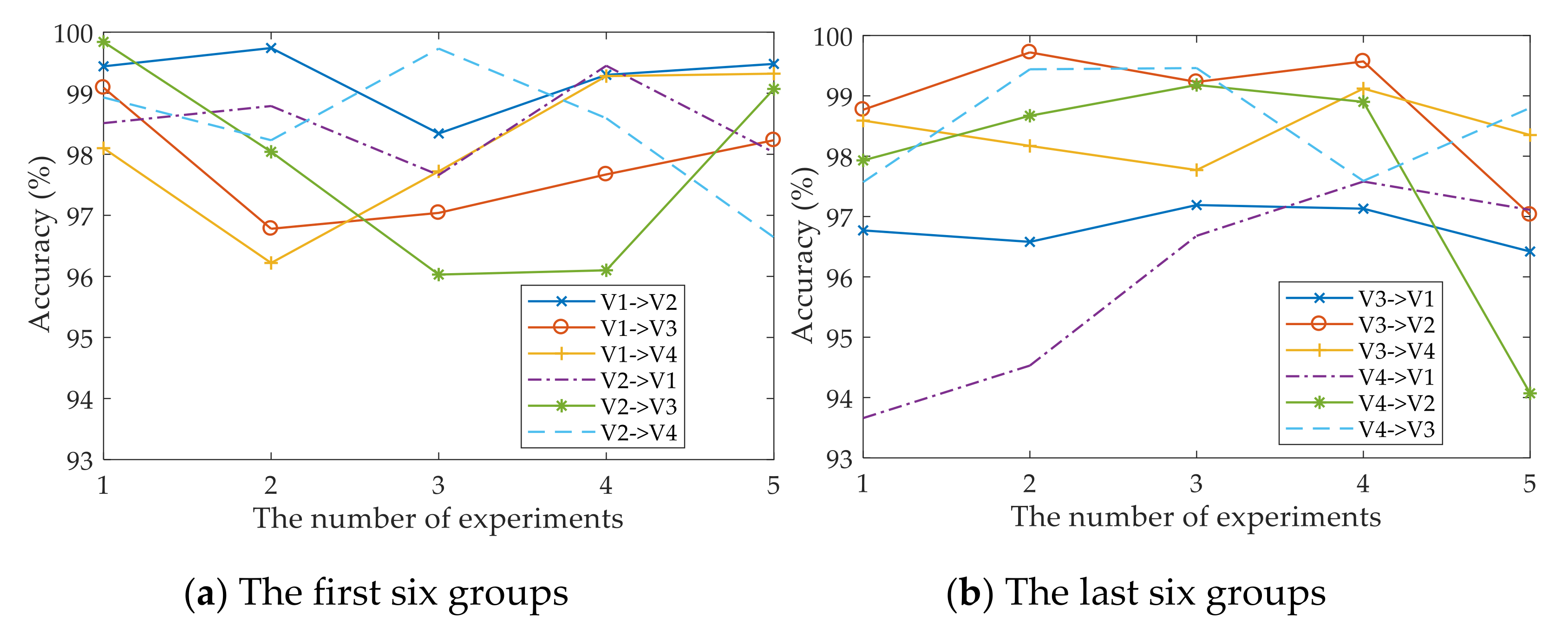
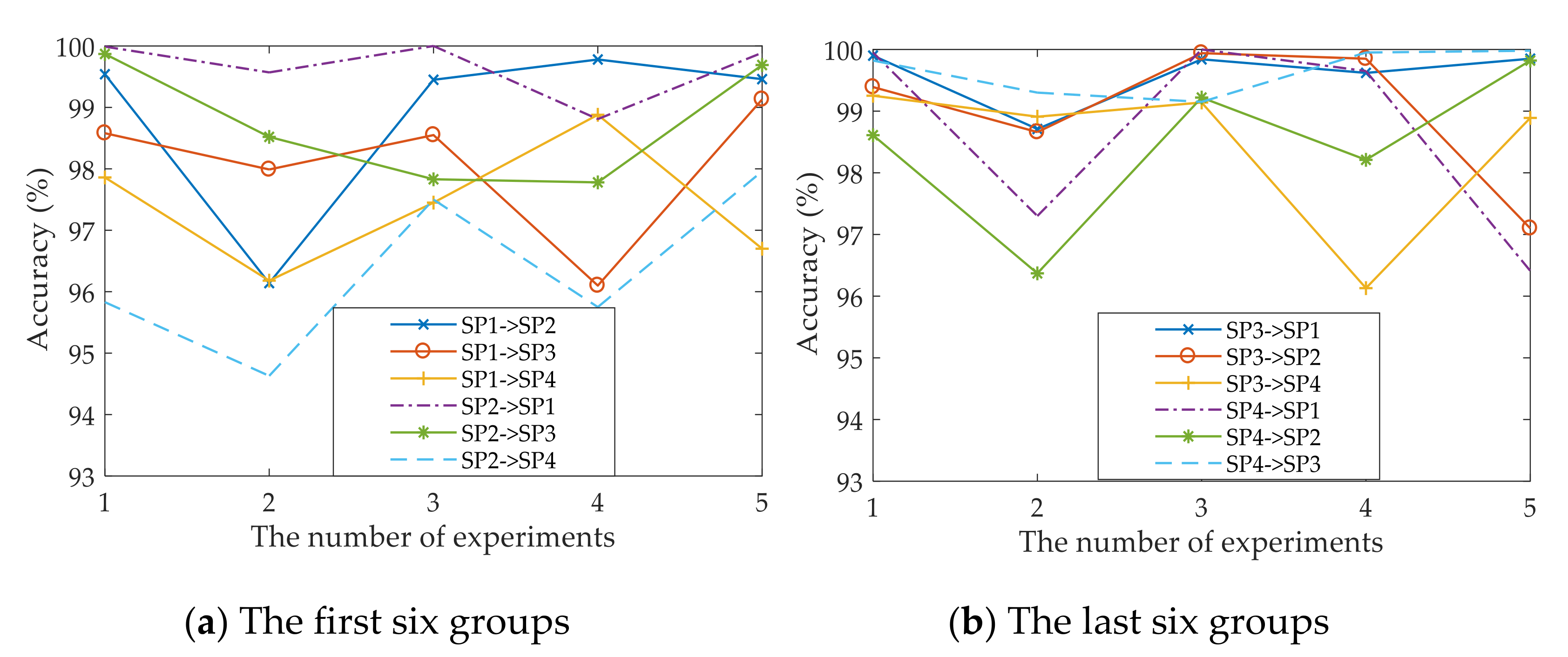
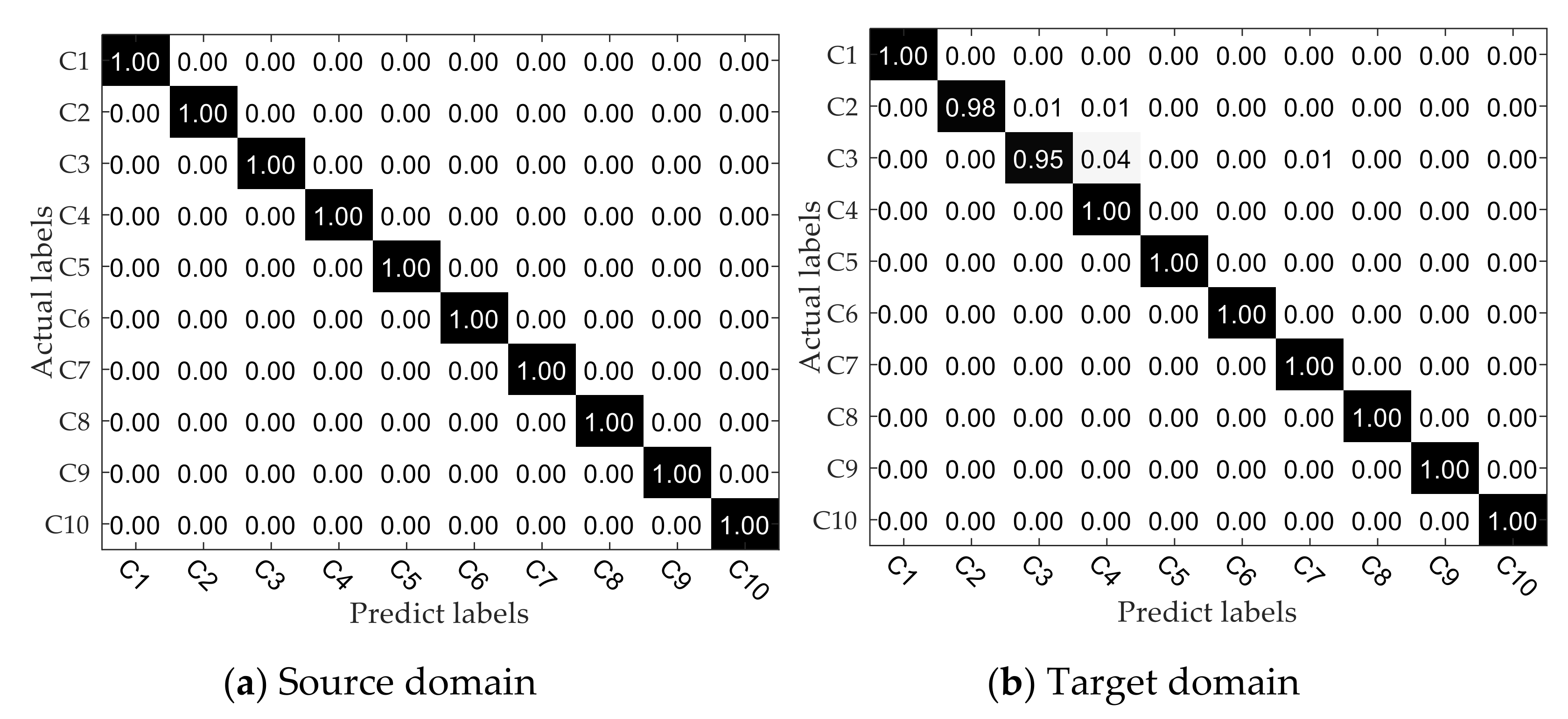
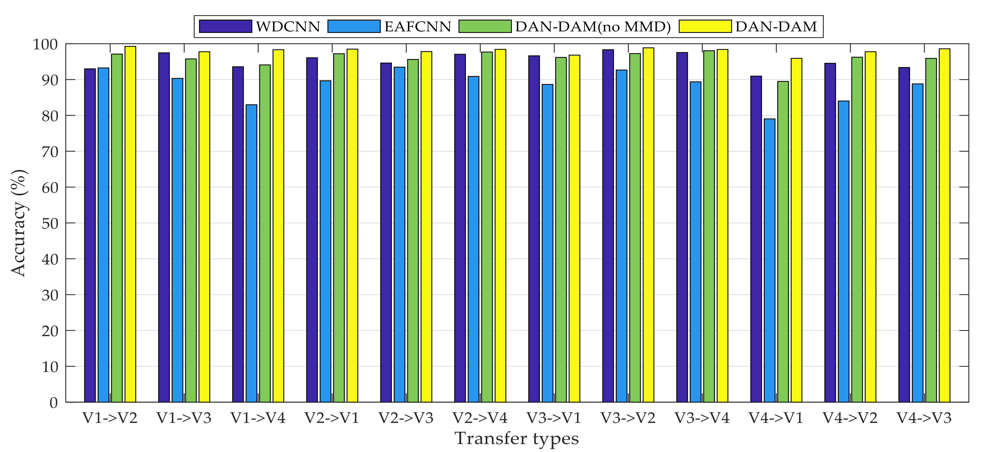
The proposed method was verified by multi-group transfer experiments and compared with other mainstream intelligent fault diagnosis methods. It can be seen from the experimental results that the DAN-DAM model has a better diagnostic effect for the domain shift samples and the diagnostic accuracy is generally higher than other mainstream diagnostic methods, which more strongly proves the superiority of the DAN-DAM model.

The rest of the paper is organized as follows: Firstly, Section 2 introduces the theoretical background of the basic knowledge involved in the proposed method. Secondly, Section 3 mainly introduces the framework of the proposed method in detail. In Section 4, the proposed model is verified experimentally to prove the diagnostic effect of the proposed method. Finally, the Section 5 gives a brief summary of the proposed method.

2. Theoretical Background

2.1. Convolutional Neural Network

The convolutional neural network (CNN) is simply the inner product operation of the image and the filter matrix. On the one hand, the CNN reduces the complexity of the model through local connection, thus reducing the risk of network overfitting; on the other hand, the CNN adopts the method of weight sharing and the number of weights is reduced, which makes it easy to optimize the network [39]. The basic structure of CNN includes a convolution layer, activation layer, pooling layer and full connection layer. The main functions of each part in CNN are as follows.

The first is the convolution layer. The main function of convolution is to extract features, so as to obtain a new set of features. The mathematical formula can be expressed as

$$z^{[l]}=W^{[l]}\ast a^{[l-1]}+b^{[l]}$$

(1)

where $a^{[l-1]}$ represents the input of layer l, $z^{[l]}$ represents the convolution output of layer l and $W^{[l]}$ and $b^{[l]}$ represent the corresponding weight and bias, respectively.

The second is the activation layer. The purpose of the activation layer is to add nonlinear factors to solve problems that the linear model cannot solve. The activation function adopts scaled exponential linear units (SELU) with its own regularization function, which can prevent network overfitting to a certain extent. The mathematical expression is as follows:

$$Z^{[l]}=SELU(z^{[l]})$$

(2)

where $Z^{[l]}$ represent the output of layer l after activation.

When the net input distribution is consistent (such as normalization to the standard normal distribution), the optimization efficiency will be improved. Therefore, batch normalization (BN) is added after the activation and the mathematical formula is simplified as follows:

$$B^{[l]}=BN(Z^{[l]})$$

(3)

Then, there is the pooling layer. The pooling layer is mainly used to select features and reduce the number of neurons in the feature mapping group, so as to reduce the dimension of features, thus avoiding network overfitting. The proposed method mainly uses two pooling functions, max pooling (max) and global average pooling (average). Max pooling is mainly used in the first few layers of CNN and global average pooling is mainly used in the last layer. The mathematical expressions are as follows:

$$h^{[l]}=\max (B^{[l]})$$

(4)

$$H^{[l]}=average(B^{[l]})$$

(5)

where $h^{[l]}$ and $H^{[l]}$, respectively, represent the outputs of the CNN after max pooling and global average pooling.

Finally, there is the full connection layer. It recombines the highly abstracted features after multi-layer convolution. Then, it carries out normalization and outputs a probability for all kinds of classification cases. Finally, the classifier can obtain classification results according to the probability obtained by full connection. Using $f^{[l+1]}$ to represent the output of the full connection layer $l+1$ and $p(x)$ to represent the probability output of Softmax, the formulas are as follows, respectively.

$$f^{[l+1]}=W^{[l+1]}{H}^{[l]}+b^{[l+1]}$$

(6)

$$p\left(x\right)=\left[p\left(C=n|x\right)\right]=\frac{\exp \left(f_n^{[l+1]}\right)}{{\displaystyle \sum _{n=1}^N\exp \left(f_n^{[l+1]}\right)}}$$

(7)

where n represents the label to which the current sample belongs and N represents all categories of the sample.

2.2. Domain Adaptation

Domain adaptation [20] is a transfer learning method to solve the problem that the source domain data distribution is different from the target domain data distribution, but the two tasks are the same. The goal is to use labeled source domain data to learn a classifier so that the unlabeled target domain can also be classified. The source domain has a large number of label samples, denoted as D_s. In the target domain, there are no label samples or a small number of label samples, denoted as D_t. Domain adaptation methods mainly include three categories: sample adaptation, feature adaptation and model adaptation. At present, the feature adaptation method is widely used due to its excellent performance, which is mainly applicable to the situation where the sample distribution in the source domain is different from that in the target domain.

Recent studies show that there are three main methods to realize feature adaptation in deep learning. The first method is based on differences, such as Kullback–Leibler (KL) divergence, Jensen–Shannon (JS) divergence and MMD. The second is an approach based on adversarial, with the help of GAN ideas. The final approach is to use batch-normalized statistics to align the source and target domain distributions into a canonical distribution. In recent years, the combination of these methods has become a hot spot for scholars from all circles to study.

2.3. Maximum Mean Discrepancy

Maximum mean discrepancy (MMD) [38] measures the distance between two distributions in a reproducing kernel Hilbert space (RKHS) and is a kernel learning method. It is the most widely used loss function to measure the distribution discrepancy between source domain and target domain in domain adaptation. The MMD distance of two distributions of source domain and target domain is

$$\mathrm{MMD}({\mathrm{D}}_{\mathrm{s}},{\mathrm{D}}_{\mathrm{t}})={\parallel \frac{1}{{\mathrm{n}}_1}{\displaystyle \sum _{\mathrm{i}=1}^{{\mathrm{n}}_1}\mathrm{\varphi }({\mathrm{x}}_{\mathrm{i}}^{\mathrm{s}})}-\frac{1}{{\mathrm{n}}_2}{\displaystyle \sum _{\mathrm{j}=1}^{{\mathrm{n}}_2}\mathrm{\varphi }({\mathrm{x}}_{\mathrm{j}}^{\mathrm{t}})}\parallel }_{\mathrm{H}}^2$$

(8)

where $\mathrm{\varphi }(.)$ stands for mapping, which is mainly used to map source domain data and target domain data to RKHS, $n_1$ and $n_2$ represent the sample numbers of source domain data and target domain data, respectively, and H indicates that this distance is measured by mapping the source and target domain data to the RKHS. It can be summarized from the above equation that the basic principle of MMD is to first project each sample in the source domain and the target domain, then sum it up and average it and, finally, use the difference between the two to represent the distribution discrepancy between the source domain and the target domain.

2.4. Wasserstein Distance

Wasserstein distance [36] is a function used to measure the distance between two probability distributions in metric space. Compared with other common measures to measure the difference of probability distribution, such as total variation, KL divergence and JS divergence, Wasserstein distance has obvious advantages. First of all, it is a natural measure of the distance between a discrete distribution and a continuous distribution. Secondly, it gives the concrete implementation scheme of transforming from one distribution to another. Moreover, finally, after the distribution changes, it can maintain the aggregate form of the distribution itself. The general mathematical expression for the Wasserstein distance is as follows:

$$W(p_1,p_2)=\underset{\gamma \in {\rm I}{\rm I}(p_1,p_2)}{\inf }{E}_{(x,y)~\gamma }[\parallel x-y\parallel ]$$

(9)

where ${\rm I}{\rm I}(p_1,p_2)$ represents the set of joint distributions of $p_1$ and $p_2$. The mathematical meaning of the formula is simply described as follows:

When $\gamma \in {\rm I}{\rm I}(p_1,p_2)$, the solution of $(x,y)$ is subject to joint distribution $\gamma$, with respect to the expectation of $\parallel x-y\parallel$, the minimum expected value of all solutions is the Wasserstein distance.

However, it is very difficult to solve the minimum expected value according to formula (9). As the centroid distribution follows an independent multivariate normal distribution, the Wasserstein distance can be calculated by the following formula:

$$W(p_1,p_2)=\sqrt{\parallel {\mu }_{p_1}-{\mu }_{p_2}{\parallel }_2^2+\parallel {\sigma }_{p_1}-{\sigma }_{p_2}{\parallel }_2^2}$$

(10)

where $\mu$ represents the mean value and $\sigma$ represents the standard deviation.

3. Proposed Method

The DAN-DAM model is composed of three parts: feature extractor, domain discriminator and double label classifiers. The basic frame diagram is shown in Figure 3 and the configuration of basic network parameters is shown in

Table 1. The parameters configuration of DAN-DAM model.

Module	Layer	Kernel Size	Stride	Channel	Pad	BN	Note
Feature extractor F	Conv-Pool1	64 × 1/2 × 1	15 × 1/2 × 1	16	Same	Yes	SELU
	Conv-Pool2	32 × 1/2 × 1	9 × 1/2 × 1	32	Same	Yes	SELU
	Conv-Pool3	16 × 1/2 × 1	9 × 1/2 × 1	64	Same	Yes	SELU
	Conv-Pool4	3 × 1/2 × 1	3 × 1/2 × 1	64	Same	Yes	SELU
	Conv-Pool5	3 × 1/1 × 1	1 × 1/1 × 1	64	Same	Yes	SELU
Label classifier1 C1	FC1	64 × 100	/	/	/	/	SELU Dropout 0.5
	FC2	100 × 10	/	1	/	/	/
	Softmax	10	/	1	/	/	/
Label classifier2 C2	FC1	64 × 120	/	/	/	/	SELU Dropout 0.5
	FC2	120 × 10	/	1	/	/	/
	Softmax	10	/	1	/	/	/
Domain discriminator D	FC1	64 × 32	/	/	/	/	SELU Dropout 0.5
	FC2	32 × 2	/	1	/	/	/
	Softmax	2	/	1	/	/	/

. The detailed introduction of each part is as follows.

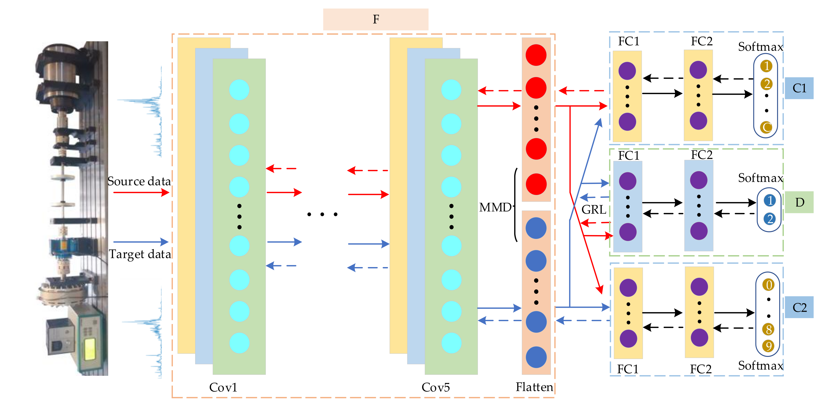
3.1. Feature Extractor

The DAN-DAM model feature extractor adopts a deep convolutional neural network (DCNN) whose composition is the same as a general shallow convolutional neural network, except that the number of convolutional layers is increased. DCNN can not only mine the general features of the signal, but also fully mine the special characteristics of the signal with the increase of the layer, getting rid of the dependence of the traditional signal processing technology on the diagnosis experience. In addition, in order to make the extracted features from the source domain and the target domain distributed consistent in the high-dimensional feature space, MMD is added to the last layer of the CNN. By minimizing the MMD distance, the feature distribution of the target domain is close to that of the source domain, which avoids the degradation learning caused by adversarial and improves the diagnostic accuracy of the network at the same time.

3.2. Domain Discriminator

Inspired by GAN, the feature extractor and domain discriminator of the DAN-DAM model are adversarial to achieve domain-level alignment. The specific adversarial process is summarized as follows: The feature extractor extracts the features of the source domain data and the target domain data, then sends the extracted features to the domain discriminator. At this time, the main function of the domain discriminator is to distinguish whether the input features are from the source domain or the target domain. However, in order to realize that the unlabeled target domain samples, which are the same as the labeled source domain samples, can also be correctly classified, the feature extractor should be updated so that the extracted features of target domain are close to the source domain, which confuses the domain discriminator and makes it impossible to identify the origin of the samples. In addition, the prerequisite for the realization of the above objective is that the two label classifiers can correctly classify the samples in the source domain. The mathematical expression of label classifier for classification is as follows:

$$L_C=-{\displaystyle \sum _{i=1}^C{\overline{y}}_i}\log y_i$$

(11)

where ${\overline{y}}_i$ represents the real label, $y_i$ is the predicted label, $L_C$ denotes the loss of the label classifier and C represents the fault category.

The mathematical expression of the domain discriminator is as follows:

$$L_D=-{\displaystyle \sum _{j=1}^2{\overline{y}}_j}\log y_j$$

(12)

where $L_D$ represents the loss of the domain discriminator.

In order to achieve the above objectives, the optimized objective function is as follows:

$$\min L_{C1}(x^s)+L_{C2}(x^s)-L_D(x^s,x^t)+L_{MMD}(x^s,x^t)$$

(13)

where $L_{MMD}$ denotes the distribution distance loss between source domain samples and target domain samples in the high-dimensional feature space.

$$\min L_{C1}(x^s)+L_{C2}(x^s)+L_D(x^s,x^t)+L_{MMD}(x^s,x^t)$$

(14)

3.3. Maximum Classifier Discrepancy

For the sake of achieving more comprehensive domain adaptation, the task-specific decision boundary should be considered at the same time to achieve class-level alignment. In the DAN-DAM model, this goal is achieved by the adversarial relationship between the feature extractor and the two label classifiers. The main steps are as follows: The first is to ensure that the two label classifiers can correctly classify the source domain samples. The second is to find the fixed feature extractor and the target domain samples far away from the source domain by maximizing the discrepancy between the two label classifiers, where the difference between the two label classifiers is realized by using Wasserstein distance. Finally, the two label classifiers are fixed and the feature extractor is updated to minimize the discrepancy between the two classifiers, so that the sample distribution of the target domain is closer to the sample distribution of the source domain. This is repeated until the unlabeled target domain samples can be correctly classified by the label classifier just like the source domain samples with the labels. The optimization objective functions, in turn, are expressed as follows:

$$\min L_{C1}(x^s)+L_{C2}(x^s)-L_W(p_1(x^t),p_2(x^t))$$

(15)

$$\min L_W(p_1(x^t),p_2(x^t))$$

(16)

where $L_W$ represents the Wasserstein distance loss.

4. Experimental Setup and Results

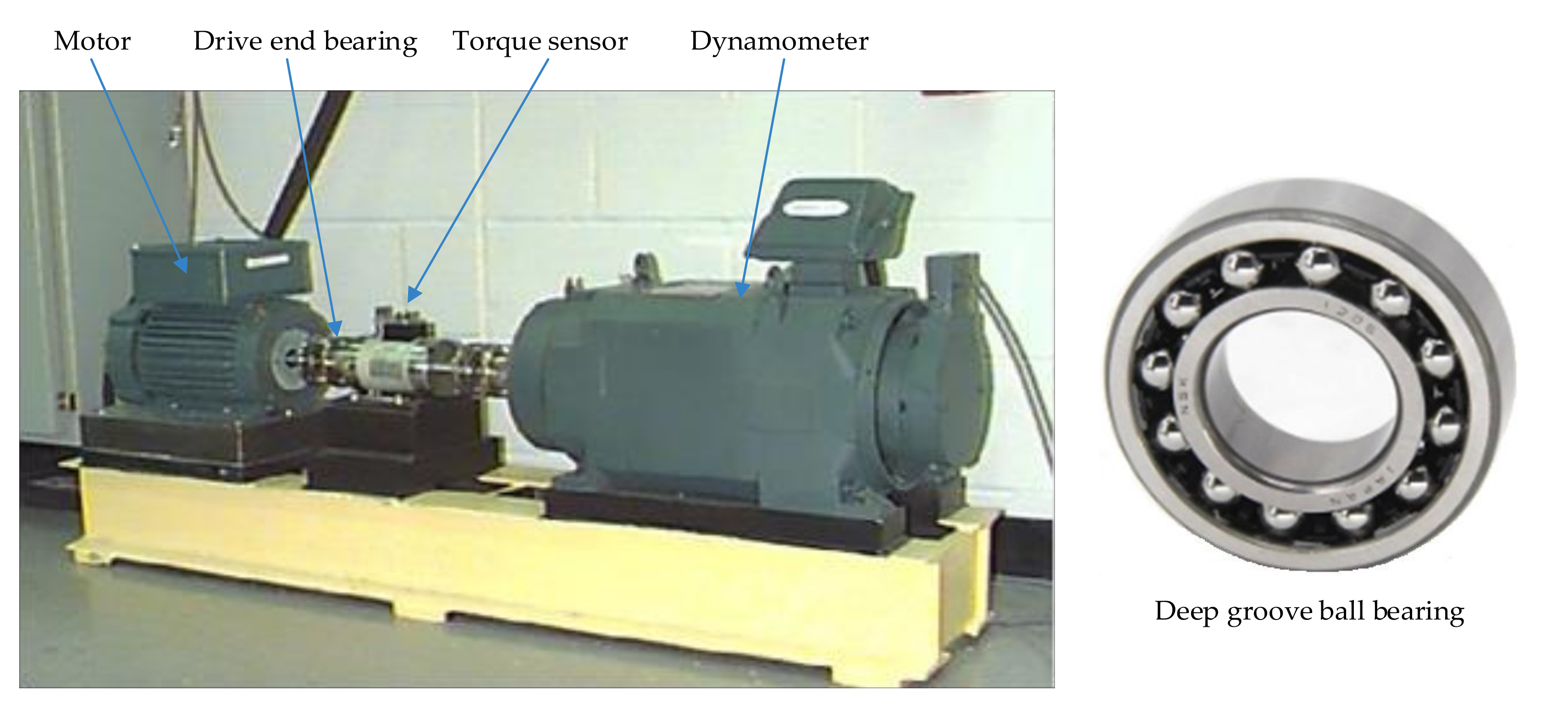
4.1. Open Datasets

To verify the validity of the DAN-DAM model, the open datasets provided by Case Western Reserve University are first used for experimental verification [40] and the experimental platform is shown in Figure 4. The experiment platform is mainly composed of four parts: motor, drive end bearing, torque sensor and dynamometer. The driving end bearing model is an SKF6205 deep groove ball bearing and 12 K driving end bearing fault data are adopted. The fault types of bearing are divided into three categories, namely, roller fault, inner race fault and outer race fault. At the same time, the data of each fault type contain three fault types with different degrees of depth: shallow (7 mil), moderate (14 mil) and severe (21 mil). Therefore, there are altogether 9 fault types of bearing, while, plus normal bearings, there are altogether 10 types of bearing data, as shown in

Table 2. Data setting parameters table of open datasets.

Fault Location	Normal	Fault in Roller			Fault in Inner Race			Fault in Outer Race
Severity (mil)	0	7	14	21	7	14	21	7	14	21
Fault abbreviation	N	RF1	RF2	RF3	IF1	IF2	IF3	OF1	OF2	OF3
Category labels	C1	C2	C3	C4	C5	C6	C7	C8	C9	C10

. Fourier transform frequency domain data are used in the transfer experiment, with 1000 data per bearing type and 600 lengths per data. Four speed types with different intervals are adopted, namely, 1730 r/min, 1750 r/min, 1772 r/min and 1797 r/min, which are represented by SP1, SP2, SP3 and SP4, successively. A total of 12 groups of different types of transfer experiments have been completed. The transfer results after the average of multiple tests of each method are shown in

Table 3. Various transfer results of four models.

Source Domain	Models	Target Domain
		SP1	SP2	SP3	SP4
SP1	WDCNN	-	85.02%	83.05%	85.78%
	EAFCNN		95.18%	86.73%	82.93%
	DAN-DAM (no MMD)		96.17%	94.38%	86.58%
	DAN-DAM (ours)		98.88%	98.07%	97.41%
SP2	WDCNN	90.22%	-	76.81%	72.21%
	EAFCNN	95.03%		96.82%	96.22%
	DAN-DAM (no MMD)	95.26%		96.22%	95.02%
	DAN-DAM (ours)	99.65%		98.74%	96.33%
SP3	WDCNN	83.69%	88.98%	-	83.88%
	EAFCNN	97.38%	98.78%		97.08%
	DAN-DAM (no MMD)	95.28%	95.21%		95.71%
	DAN-DAM (ours)	99.58%	98.99%		98.46%
SP4	WDCNN	91.10%	84.41%	86.68%	-
	EAFCNN	85.45%	98.01%	94.25%
	DAN-DAM (no MMD)	93.74%	95.43%	98.53%
	DAN-DAM (ours)	98.66%	98.45%	99.64%

.

It can be summarized, from Table 3, that, compared with the other three methods, the proposed method has the highest diagnostic accuracy in each transfer case, with the highest accuracy up to 99.65% (SP2- > SP1) and the lowest accuracy is also 96.33% (SP2- > SP4); the maximum difference of transfer results among all groups is 3.32% and the overall fluctuation is relatively small, so the model is relatively stable. The average diagnostic accuracy of DAN-DAM (no MMD) without MMD is about 4% lower than that of the DAN-DAM model under the condition of transfer in each group and the difference between the highest diagnostic accuracy and the lowest diagnostic accuracy is 11.95%, indicating relatively poor stability. Although the EAFCNN model has achieved good diagnostic results in most cases of transfer, there are several groups of poor diagnostic accuracy, lower than 87%, and the diagnostic accuracy fluctuates greatly, with the maximum difference being 15.85%. The diagnostic effect of WDCNN is the worst and the highest diagnostic accuracy is 91.01% under the transfer of each group, which is 5.32% different from the lowest diagnostic accuracy of the DAN-DAM model, and the stability is also lower than that of DAN-DAM model.

In order to further elaborate the stability of the proposed method, we draw the test results of the DAN-DAM model in the target domain for five consecutive times under each transfer condition, as shown in Figure 5. According to the analyses in Figure 5, on the one hand, the model maintains a high diagnostic accuracy in each transfer situation and most of the experimental results maintain an average of about 98%. On the other hand, looking at the output results of the same set of transfer situations for five consecutive times, the accuracy curve fluctuates relatively little and the basic fluctuation remains within 4%, so the model diagnosis effect is relatively stable.

MMD is added to the feature extraction stage of the DAN-DAM model. The main function of MMD is to align the features of the source domain and the target domain in the high-dimensional space, so that to the samples in the unlabeled target domain are gradually closer to the samples in the labeled source domain. To verify the above functions of MMD, the characteristics of output layer of the DAN-DAM model and the DAN-DAM (no MMD) model are visualized by t-SNE. SP3- > SP4 is taken as an example and the comparison of visualization results in the output layer of the two models is shown in Figure 6. As can be seen from Figure 6, the classification performance (diagnostic performance) of the DAN-DAM model is generally greater than that of the DAN-DAM (no MMD) model. The specific analysis is as follows: On the one hand, from the perspective of the classification of various types of samples, the DAN-DAM model and the DAN-DAM (no MMD) overall can distinguish various types of samples, but, with the DAN-DAM (no MMD) model, relatively many samples are mistakenly classified into other types of samples, comparing to the DAN-DAM model. For example, in Figure 6b, C3 and C4 in part overlap and, at this time, C3 is misjudged as C4. On the other hand, from the clustering effect of various types of samples, the DAN-DAM model has a better clustering effect than the DAN-DAM (no MMD) model. In the DAN-DAM model, the vast majority of samples from the same type of source domain and target domain gathers together and only a small number of samples of a few categories (three types) are outside their categories, such as C4. However, in the DAN-DAM (no MMD) model, there are four types of samples that do not have clustering and a relatively large number of samples, such as C9, are outside of the category to which they belong. To sum up, MMD can improve the diagnostic performance of the model to some extent.

Because the confusion matrix can present the classification effect of the DAN-DAM model more clearly, more explicitly and more directly, we give the confusion matrix results of SP3- > SP4 in the source domain and target domain, which are shown in Figure 7. As can be seen from Figure 7a, all types of samples in the source domain are classified 100% correctly. From Figure 7b, in the target domain, only a small number of C2 and C3 samples are misclassified, in which 1% of samples in C2 are misclassified as C3 and 1% are misclassified as C4. Moreover, 4% and 1% of the C3 samples are misclassified as C4 and C7. In addition to the above samples, all the other samples in the target domain can be classified 100% correctly. In conclusion, all the 10,000 samples are correctly classified in the source domain and only 70 samples are misclassified in the target domain. The diagnostic accuracy of the DAN-DAM model in the target domain is as high as 99.3%.

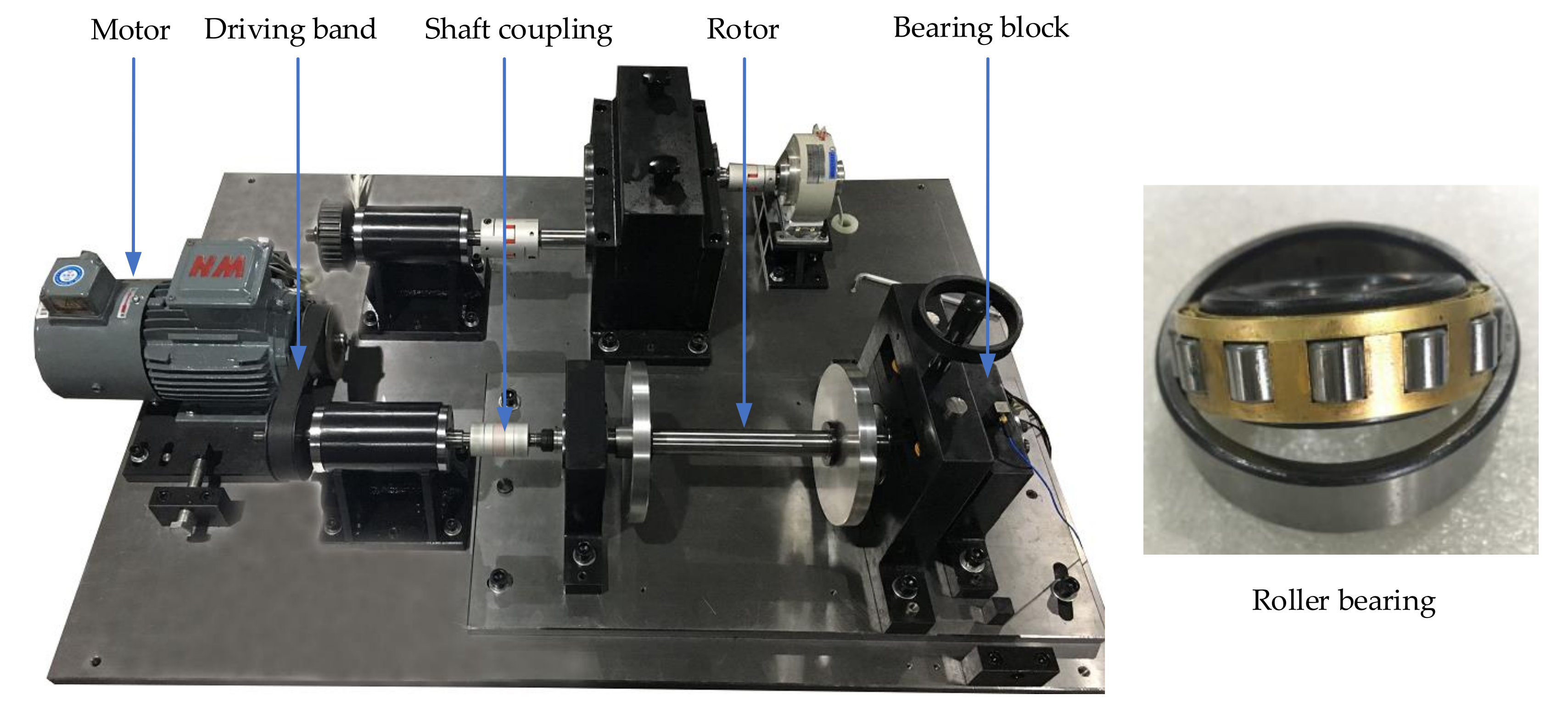
4.2. Private Datasets

We used our own experimental platform to further verify the proposed method, as shown in Figure 8. The main components include motor, driving band, shaft coupling, rotor and bearing block. The motor power is 0.75 kW, the bearing model is QPZZ-II NU205EM and the sample sampling frequency is 25.6 kHz. Fourier transform data are also used in the samples and there are four sample types: normal, roller fault, inner race fault and outer race fault—that fault depth is 0.5 mm—which are denoted by N, RF, IF and OF, respectively, as shown in

Table 4. Data setting parameters table of private datasets.

Fault Location	Normal	Fault in Roller	Fault in Inner Race	Fault in Outer Race
Severity (mm)	0	0.5	0.5	0.5
Fault abbreviation	N	RF1	IF1	OF1
Category labels	C1	C2	C3	C4

. There were also 1000 samples of each type and the length of each sample is also 600. Four different speeds are used for the transfer experiment: 1000 r/min, 1100 r/min, 1200 r/min and 1300 r/min, represented by V1, V2, V3 and V4, respectively. The comparison of diagnostic accuracy of each model under 12 different transfer conditions is shown in Figure 9.

According to the analysis of the bar chart in Figure 9, compared with other diagnostic models, the DAN-DAM model has the highest diagnostic accuracy under each transfer condition. Meanwhile, the accuracy fluctuation is relatively small, with the diagnostic accuracy of the model stable at about 97%, so the model has strong stability and generalization and the diagnostic effect is good. To more fully analyze the stability of the model, the results of five consecutive diagnoses for each transfer condition are presented, as shown in Figure 10. According to the analysis in Figure 10, for the accuracy results of five consecutive outputs of each transfer case, the accuracy fluctuation is relatively small. The vast majority of transfer cases fluctuates within 2%, while a few transfer cases fluctuates slightly large, but is also basically maintained within the range from 2% to 4%. Therefore, the DAN-DAM model is relatively stable under the same transfer condition.

The output layer of the DAN-DAM model and the DAN-DAM (no MMD) model are also features visualized by t-SNE on our own datasets. V3- > V2 is used as an example. Figure 11 shows the visualization result of t-SNE. It can be seen from the comparison between the two models that the number of overlaps between samples of different types of the DAN-DAM model is small and the number of sample misjudgments is low. Therefore, the diagnostic accuracy of the DAN-DAM model is better than that of the DAN-DAM (no MMD) model. In addition, in terms of the clustering effect, most samples of the same type in the DAN-DAM model are clustered into a cluster and only a small number of samples is not clustered with what sample types they belong, such as C2 and C3, while, in the DAN-DAM (no MMD) model, the sample gathering effect is poor and all samples of the same type are separated into multiple parts, for example, C4 has four parts. In conclusion, the addition of MMD to the model can improve the classification effect of the model, thus improving the diagnostic accuracy of the model and also, once again, verifying the function of MMD in the DAN-DAM model.

In order to more fully and specifically verify the classification ability of the proposed method, the confusion matrix diagram of the DAN-DAM model is also drawn on its own dataset, as shown in Figure 12. The overall classification ability is summarized as follows: The DAN-DAM model has achieved good classification results on its own datasets and all types of samples in the source domain can be classified 100% correctly. Except for the C2 samples on the target domain, 100% are correctly classified. In C2, 2% of the samples are misjudged as C3 and 3% of the samples are misjudged as C4. Therefore, the total number of misjudgment samples on the target domain is 50 and the total number of correctly classified samples is 3950. In summary, the fault diagnosis accuracy of the DAN-DAM model for the unlabeled target domain is 98.75%, which, once again, verifies the superior classification effect of the DAN-DAM model.

5. Conclusions

This paper proposes a DAN-DAM model for the inconsistency of sample distribution under variable working conditions. This model achieves both domain-level alignment and class-level alignment. The feature extraction stage uses a deep convolutional neural network, while using MMD to align the features of the source and target domains. The domain-level alignment is realized by adversarial of the feature extractor and the domain discriminator and, at the same time, the GRL is added to realize the automatic inversion of the gradient. Class-level alignment is achieved by using adversarial feature extractor and two classifiers, while Wasserstein distance is used to measure the difference between the two classifiers. The results of multiple different transfer experiments on two different experimental platforms show that the average diagnostic accuracy of the DAN-DAM model on the open dataset is about 98% and the average diagnostic accuracy on the private dataset is about 97%. Moreover, compared with other diagnostic models, the diagnostic accuracy is high and the stability and the generalization ability are strong.

Although the proposed method has achieved a relatively good diagnostic effect, it still has certain limitations. In the early stage, it did not consider the large discrepancy in sample distribution to train the model. We will continue to study and optimize the proposed method in the future to expand the application scope of this method.

References

1. An, Z.; Li, S.; Wang, J.; Xin, Y.; Xu, K. Generalization of deep neural network for bearing fault diagnosis under different working conditions using multiple kernel method. Neurocomputing 2019, 352, 42–53. [Google Scholar] [CrossRef]
2. Zhang, J.; Zhang, Q.; He, X.; Sun, G.; Zhou, D. Compound-Fault Diagnosis of Rotating Machinery: A Fused Imbalance Learning Method. IEEE Trans. Control. Syst. Technol. 2021, 29, 1462–1474. [Google Scholar] [CrossRef]
3. Yang, B.; Lei, Y.; Jia, F.; Xing, S. An intelligent fault diagnosis approach based on transfer learning from laboratory bearings to locomotive bearings. Mech. Syst. Signal Process. 2019, 122, 692–706. [Google Scholar] [CrossRef]
4. Yang, C.; Zhou, K.; Liu, J. SuperGraph: Spatial-temporal graph-based feature extraction for rotating machinery diagnosis. IEEE Trans. Ind. Electron. 2021, PP, 1. [Google Scholar] [CrossRef]
5. Berghout, T.; Benbouzid, M.; Mouss, L.H. Leveraging Label Information in a Knowledge-Driven Approach for Roll-ing-Element Bearings Remaining Useful Life Prediction. Energies 2021, 14, 2163. [Google Scholar] [CrossRef]
6. Li, T.; Kou, Z.; Wu, J.; Yahya, W.; Villecco, F. Multipoint Optimal Minimum Entropy Deconvolution Adjusted for Automatic Fault Diagnosis of Hoist Bearing. Shock. Vib. 2021, 2021, 1–15. [Google Scholar] [CrossRef]
7. Habbouche, H.; Amirat, Y.; Benkedjouh, T.; Benbouzid, M. Bearing Fault Event-Triggered Diagnosis using a Variational Mode Decomposition-based Machine Learning Approach. IEEE Trans. Energy Convers. 2021, PP, 1. [Google Scholar] [CrossRef]
8. Khamoudj, C.E.; Tayeb, F.B.-S.; Benatchba, K.; Benbouzid, M.; Djaafri, A. A Learning Variable Neighborhood Search Approach for Induction Machines Bearing Failures Detection and Diagnosis. Energies 2020, 13, 2953. [Google Scholar] [CrossRef]
9. Bazan, G.; Goedtel, A.; Duque-Perez, O.; Morinigo-Sotelo, D. Multi-Fault Diagnosis in Three-Phase Induction Motors Using Data Optimization and Machine Learning Techniques. Electronics 2021, 10, 1462. [Google Scholar] [CrossRef]
10. Rauber, T.W.; Loca, A.L.D.S.; Boldt, F.D.A.; Rodrigues, A.L.; Varejão, F.M. An experimental methodology to evaluate machine learning methods for fault diagnosis based on vibration signals. Expert Syst. Appl. 2021, 167, 114022. [Google Scholar] [CrossRef]
11. Tao, H.; Wang, P.; Chen, Y.; Stojanovic, V.; Yang, H. An unsupervised fault diagnosis method for rolling bearing using STFT and generative neural networks. J. Frankl. Inst. 2020, 357, 7286–7307. [Google Scholar] [CrossRef]
12. Xu, X.; Zhao, Z.; Xu, X.; Yang, J.; Chang, L.; Yan, X.; Wang, G. Machine learning-based wear fault diagnosis for marine diesel engine by fusing multiple data-driven models. Knowledge-Based Syst. 2020, 190, 105324. [Google Scholar] [CrossRef]
13. Cheng, Y.; Lin, M.; Wu, J.; Zhu, H.; Shao, X. Intelligent fault diagnosis of rotating machinery based on continuous wavelet transform-local binary convolutional neural network. Knowledge-Based Syst. 2021, 216, 106796. [Google Scholar] [CrossRef]
14. Zhao, X.; Jia, M.; Liu, Z. Semisupervised Deep Sparse Auto-Encoder with Local and Nonlocal Information for Intelligent Fault Diagnosis of Rotating Machinery. IEEE Trans. Instrum. Meas. 2021, 70, 1–13. [Google Scholar] [CrossRef]
15. Cheng, C.; Liu, W.; Wang, W.; Pecht, M. A novel deep neural network based on an unsupervised feature learning method for rotating machinery fault diagnosis. Meas. Sci. Technol. 2021, 32, 095013. [Google Scholar] [CrossRef]
16. Gai, J.; Shen, J.; Wang, H.; Hu, Y. A Parameter-Optimized DBN Using GOA and Its Application in Fault Diagnosis of Gearbox. Shock. Vib. 2020, 2020, 1–11. [Google Scholar] [CrossRef]
17. Jiang, W.; Wang, C.; Zou, J.; Zhang, S. Application of Deep Learning in Fault Diagnosis of Rotating Machinery. Processes 2021, 9, 919. [Google Scholar] [CrossRef]
18. Kolar, D.; Lisjak, D.; Pająk, M.; Gudlin, M. Intelligent Fault Diagnosis of Rotary Machinery by Convolutional Neural Network with Automatic Hyper-Parameters Tuning Using Bayesian Optimization. Sensors 2021, 21, 2411. [Google Scholar] [CrossRef]
19. Pan, S.J.; Yang, Q. A Survey on Transfer Learning. IEEE Trans. Knowl. Data Eng. 2010, 22, 1345–1359. [Google Scholar] [CrossRef]
20. Xiao, D.; Qin, C.; Yu, H.; Huang, Y.; Liu, C.; Zhang, J. Unsupervised machine fault diagnosis for noisy domain adaptation using marginal denoising autoencoder based on acoustic signals. Measurement 2021, 176, 109186. [Google Scholar] [CrossRef]
21. Lu, W.; Liang, B.; Cheng, Y.; Meng, D.; Yang, J.; Zhang, T. Deep Model Based Domain Adaptation for Fault Diagnosis. IEEE Trans. Ind. Electron. 2017, 64, 2296–2305. [Google Scholar] [CrossRef]
22. Li, X.; Jia, X.; Zhang, W.; Ma, H.; Luo, Z.; Li, X. Intelligent cross-machine fault diagnosis approach with deep auto-encoder and domain adaptation. Neurocomputing 2020, 383, 235–247. [Google Scholar] [CrossRef]
23. Singh, J.; Azamfar, M.; Ainapure, A.N.; Lee, J. Deep learning-based cross-domain adaptation for gearbox fault diagnosis under variable speed conditions. Meas. Sci. Technol. 2019, 31, 055601. [Google Scholar] [CrossRef]
24. Xu, K.; Li, S.; Jiang, X.; Lu, J.; Yu, T.; Li, R. A novel transfer diagnosis method under unbalanced sample based on discrete-peak joint attention enhancement mechanism. Knowl. -Based Syst. 2021, 212, 106645. [Google Scholar] [CrossRef]
25. Lee, K.; Han, S.; Pham, V.; Cho, S.; Choi, H.-J.; Lee, J.; Noh, I.; Lee, S. Multi-Objective Instance Weighting-Based Deep Transfer Learning Network for Intelligent Fault Diagnosis. Appl. Sci. 2021, 11, 2370. [Google Scholar] [CrossRef]
26. Xu, K.; Li, S.; Jiang, X.; An, Z.; Wang, J.; Yu, T. A renewable fusion fault diagnosis network for the variable speed conditions under unbalanced samples. Neurocomputing 2020, 379, 12–29. [Google Scholar] [CrossRef]
27. Goodfellow, I.; Pouget-Abadie, J.; Mirza, M.; Xu, B.; Warde-Farley, D.; Ozair, S.; Courville, A.; Bengio, Y. Generative Adversarial Networks. Commun. Acm 2020, 63, 139–144. [Google Scholar] [CrossRef]
28. Zhang, W.; Li, X.; Jia, X.; Ma, H.; Luo, Z.; Li, X. Machinery fault diagnosis with imbalanced data using deep generative adversarial networks. Measurement 2020, 152, 107377. [Google Scholar] [CrossRef]
29. Zheng, T.; Song, L.; Wang, J.; Teng, W.; Xu, X.; Ma, C. Data synthesis using dual discriminator conditional generative adversarial networks for imbalanced fault diagnosis of rolling bearings. Measurement 2020, 158, 107741. [Google Scholar] [CrossRef]
30. Liu, S.; Jiang, H.; Wu, Z.; Li, X. Rolling bearing fault diagnosis using variational autoencoding generative adversarial networks with deep regret analysis. Measurement 2021, 168, 108371. [Google Scholar] [CrossRef]
31. Kwon, H.; Kim, Y.; Yoon, H.; Choi, D. CAPTCHA Image Generation Systems Using Generative Adversarial Networks. IEICE Trans. Inf. Syst. 2018, E101.D, 543–546. [Google Scholar] [CrossRef] [Green Version]
32. Saito, K.; Watanabe, K.; Ushiku, Y.; Harada, T. Maximum Classifier Discrepancy for Unsupervised Domain Adaptation. In Proceedings of the 2018 IEEE/CVF Conference on Computer Vision and Pattern Recognition, Salt Lake City, UT, USA, 18–23 June 2018; pp. 3723–3732. [Google Scholar]
33. Wu, Z.; Jiang, H.; Lu, T.; Zhao, K. A deep transfer maximum classifier discrepancy method for rolling bearing fault diagnosis under few labeled data. Knowl. -Based Syst. 2020, 196, 105814. [Google Scholar] [CrossRef]
34. Li, R.; Li, S.; Xu, K.; Lu, J.; Teng, G.; Du, J. Deep domain adaptation with adversarial idea and coral alignment for transfer fault diagnosis of rolling bearing. Meas. Sci. Technol. 2021, 32, 094009. [Google Scholar] [CrossRef]
35. Guo, L.; Lei, Y.; Xing, S.; Yan, T.; Li, N. Deep Convolutional Transfer Learning Network: A New Method for Intelligent Fault Diagnosis of Machines with Unlabeled Data. IEEE Trans. Ind. Electron. 2019, 66, 7316–7325. [Google Scholar] [CrossRef]
36. Zhang, J.; Zhou, W.; Chen, X.; Yao, W.; Cao, L. Multi-Source Selective Transfer Framework in Multi-Objective Optimization Problems. IEEE Trans. Evol. Comput. 2019, 24, 1. [Google Scholar] [CrossRef]
37. Ganin, Y.; Lempitsky, V. Unsupervised domain adaptation by backpropagation. International conference on machine learning. PMLR 2015, 37, 1180–1189. [Google Scholar]
38. Xu, K.; Li, S.; Li, R.; Lu, J.; Zeng, M.; Li, X.; Du, J.; Wang, Y. Cross-domain intelligent diagnostic network based on enhanced attention features and characteristics visualization. Meas. Sci. Technol. 2021, 32, 114009. [Google Scholar] [CrossRef]
39. Poria, S.; Cambria, E.; Gelbukh, A. Aspect extraction for opinion mining with a deep convolutional neural network. Knowl. -Based Syst. 2016, 108, 42–49. [Google Scholar] [CrossRef]
40. Smith, W.; Randall, R. Rolling element bearing diagnostics using the Case Western Reserve University data: A benchmark study. Mech. Syst. Signal. Process. 2015, 64–65, 100–131. [Google Scholar] [CrossRef]
Figure 1. The general frame diagram of domain adaptation.
Applsci 11 07983 g001
Figure 2. Classification comparison of various domain adaptation methods.
Applsci 11 07983 g002
Figure 3. Basic frame diagram of DAN-DAM model.
Applsci 11 07983 g003
Figure 4. The experiment platform of Case Western Reserve University.
Applsci 11 07983 g004
Figure 5. The five consecutive test results of the DAN-DAM model in diverse transfers for open datasets.
Applsci 11 07983 g005
Figure 6. Feature visualization via t-SNE in output layers for open datasets.
Applsci 11 07983 g006
Figure 7. The confusion matrix of the DAN-DAM model in two domains for open datasets.
Applsci 11 07983 g007
Figure 8. The experiment platform of private datasets.
Applsci 11 07983 g008
Figure 9. Various transfer results of four models.
Applsci 11 07983 g009
Figure 10. The five consecutive test results of the DAN-DAM model in diverse transfers for private datasets.
Applsci 11 07983 g010
Figure 11. Feature visualization via t-SNE in output layers for private datasets.
Applsci 11 07983 g011
Figure 12. The confusion matrix of the DAN-DAM model in two domains for private datasets.
Applsci 11 07983 g012