Article

Investigating Rural Single-Vehicle Crash Severity by Vehicle Types Using Full Bayesian Spatial Random Parameters Logit Model

1
School of Transportation and Vehicle Engineering, Shandong University of Technology, Zibo 255000, China
2
Center for Urban Transportation Research, University of South Florida, Tampa, FL 33620, USA
*
Author to whom correspondence should be addressed.
Appl. Sci. 2021, 11(17), 7819; https://doi.org/10.3390/app11177819
Submission received: 4 August 2021 / Revised: 20 August 2021 / Accepted: 22 August 2021 / Published: 25 August 2021

Abstract

:
The effect of risk factors on crash severity varies across vehicle types. The objective of this study was to explore the risk factors associated with the severity of rural single-vehicle (SV) crashes. Four vehicle types including passenger car, motorcycle, pickup, and truck were considered. To synthetically accommodate unobserved heterogeneity and spatial correlation in crash data, a novel Bayesian spatial random parameters logit (SRP-logit) model is proposed. Rural SV crash data in Shandong Province were extracted to calibrate the model. Three traditional logit approaches—multinomial logit model, random parameter logit model, and random intercept logit model—were also established and compared with the proposed model. The results indicated that the SRP-logit model exhibits the best fit performance compared with other models, highlighting that simultaneously accommodating unobserved heterogeneity and spatial correlation is a promising modeling approach. Further, there is a significant positive correlation between weekend, dark (without street lighting) conditions, and collision with fixed object and severe crashes and a significant negative correlation between collision with pedestrians and severe crashes. The findings can provide valuable information for policy makers to improve traffic safety performance in rural areas.

1. Introduction

Different from developed countries, there is serious latent danger in rural areas of China, such as a complex traffic environment, inadequate infrastructure, high speed, and sluggish rescue response. These adverse factors increase the possibility of serious traffic crashes. In 2017, the number of traffic crashes and fatalities in rural areas in China accounted for 48.43% and 40.59% of the respective totals for all crashes [1]. Thus, rural crashes have been considered a fatality-concentrated event, especially for rural single-vehicle (SV) crashes.
Rural SV crashes usually have serious consequences; the number of fatalities has increased significantly in recent years, showing an average growth rate of 4.8% from 2013 to 2017. Further, there were 24 rural crashes resulting in 10 or more fatalities, including 20 SV crashes [1]. Hence, transportation professionals were encouraged to explore the risk factors of SV crash severity in rural areas.
Identifying the risk factors of rural SV crash severity are helpful to improve traffic safety on rural roadways. According to the characteristics of risk factors, targeted measures can be taken. Hence, numerous severity prediction functions (SPFs) were established [2,3]. However, existing research does not distinguish different motor vehicle types during the crash severity modeling process.
There are many types of motor vehicles, such as passenger car, motorcycle, pickup, and truck, each with its own characteristics. It is expected that the influence of risk factors on the severity of rural SV crashes may vary across different vehicle types. If the same SPFs were used for different vehicle types, the variability of crash mechanisms will be ignored and will also lead to unsatisfactory prediction performance. Conversely, modeling of rural SV crashes based on different vehicle types is expected to overcome these deficiencies and can help to visualize the variant impacts of risk factors on crash severity.
In addition, as a crash is the result of many factors, there are always some unobserved or unobservable factors that will affect crash severity, named unobserved heterogeneity [4,5]. Ignoring unobserved heterogeneity may lead to erroneous parameter inference [6].
To capture the effects of unobserved heterogeneity on the severity of rural SV crashes, several heterogeneity models have been constructed [7,8], such as random parameters logit model and random intercept logit model. These models allow parameters to vary across observations, which provides a flexible framework. Theoretically, they can simulate all selection patterns based on probabilistic propensities [9,10]. However, such approaches cannot capture the spatial correlation across crashes, which will limit the promotion of the model. Importantly, the spatial correlation of adjacent crashes has been commonly recognized in crash rates, crash counts, and traffic conflict analyses [2,11], but this issue is often overlooked in crash severity analyses, especially for rural SV crashes, which may lead to the prediction accuracy being substantially undermined.
Based on the above analysis, it is meaningful to establish statistical models across motor vehicle types for rural SV crash severity and to simultaneously accommodate the unobserved heterogeneity and spatial correlation. The research results are helpful to clarify the variable influences of risk factors on rural SV crash severity and create a safer transportation environment in rural areas.
The rest of this paper is organized as follows. A comprehensive literature review for rural SV crash analysis is given in Section 2. Section 3 provides detailed information on the studied crash dataset. The methodological framework in this research is presented in Section 4, and analysis and discussion of the estimation results are given in Section 5. Conclusions and potential limitations of this research are described in Section 6 and Section 7, respectively.

2. Literature Review

2.1. Covariates Analysis of Rural Single-Vehicle Crashes

Due to fatality-concentrate, rural SV crashes have attracted extensive interest from transportation professionals, and various risk factors have been explored. These factors can be divided into four components—driver characteristics, crash-specific characteristics, environmental characteristics, and temporal characteristics.

2.1.1. Driver Characteristics

Numerous studies have shown that driver-related characteristics have a significant influence on the severity of rural SV crashes, including lack of seat belt use, drunk driving, speeding, fatigue, driver age, and driver gender. For example, the probability of fatal crashes in rural areas due to seat belts not being used and drunk driving will increase 15.3% and 36.3%, respectively [12]. It was also suggested that fatigue is associated with severe rural SV crashes and that increasing rest breaks could reduce crash risk [13,14]. Driver age was divided into three stages—young drivers (age < 24), mid-age drivers (24–65), and older drivers (age > 65)—to establish SPFs, suggesting that the probability of severe crashes varied across age stages [15]. Specifically, compared with mid-age drivers, the probability of serious crashes of young drivers was reduced by 4.8% and that of old drivers was increased by 66.2% [16].
There is a significant correlation between driver gender and crash severity, which has been widely accepted. However, due to the differences of research objects and modeling methods, inconsistent findings have been shown. A partial proportionality odds model and a mixed logit model were established using SV run-off-road crashes to investigate the factors associated with crash severity. It was found that male drivers were more likely to be involved in fatal or severe crashes than female drivers [17,18]. Subsequently, a hierarchical Bayesian random intercept approach and a random parameter hierarchical ordered probit approach were established and found that female drivers were more likely to be involved in serious crashes than males [19,20]. Further, weather conditions were divided into five categories—sun, rain, snow, fog, and overcast—to capture risk factors. The regression results suggested that male drivers were more likely to be involved in fatal or severe crashes in sunny and snowy weather than females, but this finding could not be supported by rainy, foggy, and overcast weather [21]. These findings suggest that there is no definite conclusion about the impact of driver gender on crash severity. This may be related to the effect of unobserved heterogeneity on regression results.

2.1.2. Crash-Specific Characteristics

According to previous studies, the severity of rural SV crashes will vary across crash type (e.g., collision with fixed object, rollover/overturn, collision with pedestrian, collision with animal) [22]. Collision with a fixed object will increase the probability of serious crashes by 72.2% compared to collision with a non-fixed object [16]. A similar finding can be found in other studies [13,23]. In particular, collisions resulting in motor vehicle overturning were more likely to have serious crash consequences [24]. It is generally known that animals and pedestrians are vulnerable to motor vehicles; collisions between motor vehicles and animals or pedestrians usually do not adversely affect drivers, but they can easily take the lives of animals or pedestrians [25].
Similarly, crash severity is expected to vary across different motor vehicle types, which are commonly accommodated as candidate risk factors and combined with other factors [26,27]. Three motor vehicle categories—large vehicle, passenger vehicle, and motorcycle—were included to establish ordered logistic regression, suggesting that the consequences of motorcycle crashes were more severe compared with large vehicle crashes, followed by passenger car crashes [24]. In addition, passenger car crashes and pickup crashes were negatively correlated with crash severity [16,28].

2.1.3. Environmental Characteristics

Several traffic characteristics, such as speed limit and traffic volume, were demonstrated to be significantly correlated with rural SV crash severity [29,30]. In detail, crashes occurring on roadways with speed limits below 35 mph or AADT (Annual Average Daily Traffic) above 5000 were more likely to result in less serious injury outcomes due to a safe speed being maintained under car-following conditions [31].
Existing studies have shown that there is a negative correlation between adverse environmental conditions and crash severity [17,18,30]. It is believed that the reduction of injury severity is attributable to more careful driving in bad environments. Some contradictory findings were also demonstrated, namely that crashes occurring in rainy and snowy weather could lead to severe consequences [29]. Some speed limit measures have been considered to reduce crash severity under inclement weather [32,33,34]. Meanwhile, in dark without streetlights conditions, SV crashes are more likely to cause serious injuries [17].

2.1.4. Temporal Characteristics

Drivers are more prone to be fatigued or sleepy in the early morning, a risky behavior that will have a deleterious effect on traffic safety. Both the frequency and severity of crashes show an increased trend [17]. In addition, rural SV crashes occurring between 6:00 p.m. and 12:00 p.m. are unlikely to result in serious injury [29,31]. The same research suggested that serious crashes were more likely to occur during the winter season.
Further, the probability of severe crashes on weekdays was higher than on weekends [17,35]. It was also pointed out that if off-duty time exceeds 46 h, such as more than a weekend, the risk of crashing will increase when a driver returns to work [36].

2.2. Statistical Techniques for Crash Severity

2.2.1. Unobserved Heterogeneity in Crash Analysis

Considering the discrete characteristics of crash severity outcome, several discrete choice models have been introduced. One of the most commonly used analysis techniques is a logit approach. Among various logit approaches, the multinomial logit (MN-logit) model has been widely used due to its simple structure and easy-to-read parameters. For example, the MN-logit model was calibrated to analyze the risk factors of motorcycle crashes and pedestrian–vehicle crashes, respectively [37,38]. Subsequently, a binary logit model was employed to fit roadside accidents and suggested that rural crashes should be investigated separately [22]. However, the parameters of the MN-logit model are fixed, which cannot identify the unobserved heterogeneity. This regression pattern may not be able to exhibit the real contribution of risk factors on crash severity. Therefore, some advanced modeling techniques, such as random parameters logit (RP-logit) model and random intercept logit (RI-logit) model, have been recommended.
The RP-logit model is a discrete choice model with high flexibility and adaptability that captures the unobserved heterogeneity by allowing parameters to vary across observations. This statistical technique has been known for many years, but it was not fully applicable until the advent of simulation technology. Up to now, it has developed into a satisfactory approach for estimating crash severity [2,9]. Milton et al. [39] were among the first to employ the RP-logit model in accident analysis and suggested that this approach can be used to verify the distribution of crash severity on roadway segments. Subsequently, the pedestrian injury severity in pedestrian-vehicle crashes was investigated. It was found that the effect of pedestrian age on injury severity was normally distributed across crashes and the probability of fatal injury increased significantly with the increase of pedestrian age [25,40].
More specifically, the RI-logit model can be regarded as a special form of the RP-logit model, which addresses the unobserved heterogeneity by allowing model intercept to vary across individual crashes [11]. Xu et al. [41] used the RI-logit model for traffic safety analysis earlier. Based on crash data of I–880N in California, crash risk prediction models were developed for different weather conditions, and the influence of traffic flow variables on crash risk was captured. It was found that model predictive performance can be effectively improved by allowing the model intercept to vary across observations. Additionally, a hierarchical Bayesian approach was proposed to examine the posterior probability of driver injury severity in rural truck-related crashes [42]. The results indicated that capturing random effects plays an important role in predicting injury outcomes.

2.2.2. Spatial Correlation in Crash Analysis

Currently, spatial statistical techniques have been highly praised. For example, the risk factors associated with freeway crashes were explored by developing a spatial generalized ordered logit model [43]. The results showed that there were several important factors affecting freeway crash severities, such as vehicle type, season, traffic volume, crash type, and driver experience. Further, the spatial correlation effect was accommodated using a spatial structure error term to investigate the risk factors of crash frequency [44]. The results showed that the model simultaneously considering spatial correlation and unobserved heterogeneity outperforms the model considering only unobserved heterogeneity. The same conclusion was obtained by Klassen et al. [45], who used a spatial random intercept model to explore bicycle-motor vehicle crashes. In addition, there are many other studies to determine the risk factors of injury outcomes by establishing statistical functions with spatial error term [46,47,48]. That research could provide inspiration for this research.
The existing spatial crash severity functions evolved from traditional statistical techniques by constructing a spatial structure term, including the MN-logit model, RI-logit model, and ordered logit model, etc. The spatial statistical function developed from a random coefficient model is limited. Numerous research studies have demonstrated that random coefficient regression functions are superior statistical techniques to fixed coefficient functions [2]. Hence, constructing a spatial structure in a random coefficient function is expected to exhibit a superior regression performance. Lately, some inspiring spatial random parameters functions have been established, including spatial random parameters Poisson-lognormal regression and spatial random parameters Tobit regression [49,50]. These models were used to investigate crash frequency and crash rate, respectively. Based on an in-depth review of crash severity studies, few spatial random coefficient models were found that could fit crash severity. This is a methodological gap in traffic safety analysis and corresponding research should be conducted to enrich statistical theory.

2.3. The Current Research
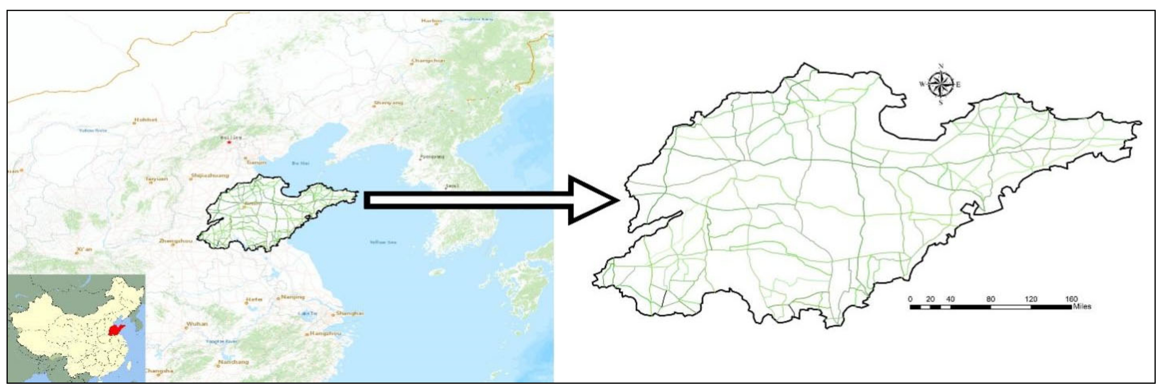
Unobserved heterogeneity and spatial correlation have been widely recognized in accident analysis. Due to the substantial differences between different motor vehicle types, these two characteristics are expected to vary across vehicle types. Hence, this research was conducted to comprehensively accommodate the unobserved heterogeneity and spatial correlation by vehicle types in rural SV crashes to clarify the variable and interesting relationship between risk factors and injury severity. A novel spatial random parameters logit (SRP-logit) model with spatial and unstructured error terms is proposed. Three candidate models—MN-logit model, RP-logit model, and RI-logit model—were also calibrated under the Bayesian framework and compared with the proposed model. Meanwhile, several risk factors of crash severity across different vehicle types were identified. This study provides a reference for traffic safety researchers to determine a satisfactory statistical approach and provides valuable risk factors across vehicle types for traffic managers to improve rural traffic safety.

3. Data

This study focused on the analysis of crashes on a rural two-lane highway without divider or signal controls in Shandong Province, China. In total, 110 rural highways were selected. A map of the study area is shown in Figure 1. SV crashes related to four motor vehicle types (passenger car, motorcycle, pickup, and truck) from 2015 to 2020 were collected to calibrate the crash model. The studied dataset was composed of the information from three different data sources—(1) a crash database extracted from the Crash Reporting System maintained by the Traffic Administration Bureau of Shandong Department of Public Security; (2) a real-time meteorological dataset collected from the Meteorological Information Management System maintained by Shandong Climate Center; and (3) a geographic dataset of the target road derived from the Traffic Information System maintained by the Shandong Department of Transportation. A total of 29,814 crashes were integrated. After removing data with key information errors, 29,525 crashes were employed for subsequent modeling.
In this research, crash severity and various risk factors were identified as dependent and independent variables, respectively. Both the dependent and independent variables were transformed into discrete variables to fit the regression functions. Generally, there are three methods to determine the crash severity: (1) based on driver injury severity [51]; (2) based on most seriously injured passengers [52]; and (3) based on most serious injury in a crash [53]. Given the substantial differences in safety awareness among passengers as well as between drivers and passengers, the latter two approaches may introduce some additional heterogeneity. Thus, to reduce the potential heterogeneity and improve the reliability of model parameters, driver injury severity was used to measure crash severity for subsequent regression analysis.
In the database, crash-related driver injuries were classified into four categories—no injury (70.0%), slight injury (20.1%), serious injury (7.8%) and fatal injury (2.1%). A driver passing away within seven days was regarded as a fatal event. Fatality cases were very limited in the dataset, which may lead to incorrect inference. Considering that the two adjacent injury categories are similar, the combination of fatality and serious injury, called FS injuries, was not expected to have a substantial impact on parameters estimation [54,55]. Thus, the dependent variable was a tripartite injury result (no injury, slight injury, FS injuries), in which the interest response refers to FS injuries, and no injury was considered as reference variable.
Descriptive statistics of dependent variables across vehicle types are shown in Figure 2. As shown, a similar proportion of injury severity was maintained by passenger car, pickup, and truck crashes. The percentages of no injury for passenger car, pickup, and truck crashes were 87.7%, 87.0%, and 88.5%, respectively, followed by slight injury (9.6%, 9.4%, and 6.9%, respectively) and FS injuries (2.7%, 3.6% and 4.6%, respectively). Further, there is a significant difference in the proportion of injury severity between motorcycle crashes and other motor vehicle crashes. The percentage of slight injury (57.5%) was highest in motorcycle crashes, followed by FS injuries (23.7%) and no injury (18.8%). This may be related to the fact that motorcycle cannot provide adequate protection for riders.
Several risk factors, including driver gender, driver age, drunk driving, weather, road surface, crash type, week, month, season, light, crash time and traffic control, were recorded in the crash dataset. Among them, some continuous variables, such as age, month, and crash time, were discretized. Driver age was divided into three categories, including young driver (<30), middle-aged driver (30–60), and older adult driver (>60). Middle-aged driver was identified as the reference variable. The month was also divided into three categories (early in month, middle of month, and late in month). Note that the beginning of the month and the middle of the month represent the 1st to 10th and the 11th to 20th of each month; late in the month represents the remaining days of the month. Crash time was transformed into a binary discrete variable, including day and night. Among them, daytime was used as a reference variable.
Further, the categorical variables in the raw data were reasonably combined to slim down the model. More specifically, rain, snow, and fog were combined as non-clear weather; hence, clear and non-clear identified the weather condition. Driver gender and drunk driving were determined based on traffic police records and were classified as binary variables. Wet pavement, muddy pavement, and snowy pavement were combined as non-dry road surface; two categories—dry and non-dry pavements—were shown as road surface conditions. More than 20 crash types were recorded in the raw data that were combined into four categories—collision with fixed object, collision with non-fixed object, collision with pedestrian, and other. Similar independent variable classification can be found in Wei et al. [51]. Lighting conditions were divided into three categories—daylight, dark (with street lighting), and dark (without street lighting)—to explore the impact of risk factors on crash severity across different vehicle types. In addition, several traffic control modes are included in the original records, such as traffic lights, police direction, speed limit monitoring, and other traffic infrastructure. These traffic control modes were marked as traffic control, otherwise marked as no traffic control. The descriptive statistics of the independent variables are shown in Table 1.
From Table 1, it can be seen that the proportion of risk factors varies with the types of motor vehicles. In detail, the proportions of female drivers in passenger car, motorcycle, pickup, and truck crashes were 13.7%, 7.2%, 6.1%, and 0.2%, respectively, highlighting a trend of gradual decrease. Furthermore, motorcycle crashes had higher percentages of older adult drivers (35.4%) than crashes of any other vehicle type, 14.8% for passenger car, 14.0% for pickup, and 10.6% for truck. Drunk driving was found to have similar effect on percentage value in crashes of the four vehicle types—25.8% for motorcycle, 15.0% for passenger car, 9.1% for pickup, and 0.6% for truck.
However, a completely different phenomenon is represented by collision with fixed object. The proportion of collisions with fixed object related to truck crashes was 17% and was the highest, followed by motorcycle (11.2%), passenger car (7.3%), and pickup crashes (6.4%). The proportion of dark (without street lighting) condition in different motor vehicle types remained largely consistent with collision with fixed object. Finally, the ratio of weather, road surface, week, month, season, and traffic control remained basically consistent among different vehicle types.
These statistics showed that the proportion of risk factors varies significantly across different vehicle types, which may lead to unstable regression coefficient; thus, it is necessary to investigate different vehicle types separately.
Of note is that the proportion of some variables in Table 1 is less than 1%, such as female driver and drunk driving involved in truck crashes. These variables may lead to unstable model estimation and were eliminated.

4. Methodology

As discussed, the driver injury severity of a rural SV crash is specified to be one of three discrete categories—no injury, slight injury, and FS injuries. Given these three discrete crash severity levels, statistical models can be derived that can be used to determine the probability of a vehicle crash with a specific severity level. To verify the differences of fit performance between different crash severity models and identify the factors that have a significant influence on the severity of rural SV crashes, four logit models were constructed under the Bayesian framework, including the MN-logit model, the RP-logit model, the RI-logit model, and the SRP-logit model. The specific model structures are as follows.

4.1. Model Specifications

4.1.1. Multinomial Logit Model

The MN-logit model formulation was discussed in Shankar and Mannering [56]. For a given dataset of rural SV crashes, the probability of driver injury level k in crash i is given as:
P i , k w = P ( U i , k w U i , j w )    k j ,
where P i , k w denotes the probability of ith crash with injury level k on the wth road segment; j is the set of possible injury severities; U i , k w is a propensity function of covariates that determines the likelihood of crash i resulting in crash severity k. To clarify this likelihood, a function that defines the severity probability needs to be specified and a linear function was assumed:
U i , k w = β k X i w + ε i , k ,
β k X i w = β k , 0 + β k , 1 x i , 1 w + β k , 2 x i , 2 w + + β k ,   L x i , L w = β k , 0 + l = 1 L β k , l x i , l w ,
where X i w is a vector of independent variables, such as driver gender, driver age, drunk driving, weather, road surface, etc., which determines the injury outcome k; x i , l w is the value of predictive variable l for ith crash; β k denotes a vector of estimable coefficient corresponding to the injury outcome k; β k , l is the coefficient of the predictive variable l; β k , 0 denotes the model intercept; ε i , k is an error term, which follows type I extreme value distribution.
As noted, the dependent variable was a tripartite injury result; hence, we have Y i w = ( Y i , 1 w , Y i , 2 w ,   Y i , 3 w ) ; Y i w = 1 denotes no injury and was considered as the reference category, while Y i w = 2 and Y i w = 3 indicate slight injury and FS injuries, respectively. Let P i , k w = P r Y i w = k denote the probability of Y i w = k . Therefore, we have:
Y i w ~ categorical ( P i , 1 w , P i , 2 w , P i , 3 w ) .
Assuming that the probabilities ( P i , 1 w ,   P i , 2 w ,   P i , 3 w ) of crash severity obey a multinomial logistic distribution, the structure of MN-logit model can be shown as follows.
logit P i , k w = log P i , k w P i , 1 w = β k , 0 + l = 1 L β k , l x i , l w ,   ( k = 2 ,   3 ) ,
where all variables in Equation (5) are the same as those defined earlier.

4.1.2. Random Parameters Logit Model

The MN-logit model believes that the impact of predictors remains constant for all crashes. This phenomenon violates the fact that the influence of risk factors may vary across observations [16]. Hence, the RP-logit model was established by setting the fixed parameters β k , 0 ,   β k , 1 ,   ,   β k , L in the MN-logit model to be random parameters β i , k , 0 ,   β i , k , 1 ,   ,   β i , k , L to accommodate the variable influence of risk factors on crash severity. We have:
logit P i , k w = log P i , k w P i , 1 w = β i , k , 0 + l = 1 L β i , k , l x i , l w ,   ( k = 2 ,   3 ) .
Assuming that the possible random coefficients are normally distributed as β i , k ~ N ( μ k ,   φ k ) , where:
β i , k = β i , k 0 β i , k 1 β i , k L ,   μ k = μ k 0 μ k 1 μ k L ,   φ k = ( φ 0 , 0 k ) 2 ( φ 0 , 1 k ) 2 ( φ 0 , L k ) 2 ( φ 1 , 0 k ) 2 ( φ 1 , 1 k ) 2 ( φ 1 , L k ) 2 ( φ L , 0 k ) 2 ( φ L , 1 k ) 2 ( φ L , L k ) 2 .
The diagonal element φ l , l k 2 is the variance of random parameter β i , k , l . The off-diagonal element φ l 1 , l 2 k 2 ,   ( l 1 l 2 ) is the covariance between β i , k , l 1 and β i , k , l 2 .
The model coefficient is regarded as random across observations if the posterior estimation variance is different from zero at a significance level of 10%. Otherwise, the coefficient is treated as fixed across observations.

4.1.3. Random Intercept Logit Model

The RI-logit model is a special form of the RP-logit model and only allows the intercept to vary randomly across individual observations. It is not as flexible as the RP-logit model, but it is also widely accepted by traffic safety professionals [41,42,57].
The structure of RI-logit model can be expressed as:
logit P i , k w = log P i , k w P i , 1 w = β i , k , 0 + l = 1 L β k , l x i , l w ,   ( k = 2 ,   3 ) .
The intercept β i , k , 0 is set as a random parameter across observations and follows a normal distribution as:
β i , k , 0 ~ N ( μ k , 0 , σ k , 0 2 ) .

4.1.4. Spatial Random Parameters Logit Model

Both the RP-logit model and the RI-logit model can identify the unobserved heterogeneity across crashes effectively. Nevertheless, some critical issues still need to be resolved. A typical representative is to identify the spatial correlation of crashes. Hence, the SRP-logit model was proposed to comprehensively accommodate the spatial correlation and unobserved heterogeneity and the derivation process is as follows.
To address the potential variations across road segments, an unstructured error term was constructed. The RP-logit model can be modified to:
logit P i , k w = log P i , k w P i , 1 w = β i , k , 0 + l = 1 L β i , k , l x i , l w + u k w ,   ( k = 2 ,   3 ) u k w ~ N ( 0 ,   σ u k 2 ) ,
where the error term u k w was accommodated to permit the potential within-segment correlation and cross-segment heterogeneity and followed normal distribution. σ u k 2 represents the variance of unstructured error term.
In most cases, the existence of spatial correlation is reasonable because the adjacent segments will have similar geometric features and environments [47,54]. This may lead to certain factors shared among adjacent crashes [11]. As demonstrated by El-Basyouny and Sayed [58], random variations across sites may be structured spatially due to the complexity of traffic interactions around crash sites. To this end, a structured spatial error term s k w was included in the regression function, resulting in the final SRP-logit model:
logit P i , k w = log P i , k w P i , 1 w = β i , k , 0 + l = 1 L β i , k , l x i , l w + u k w + s k w ,   ( k = 2 ,   3 ) .
An effective and commonly used joint density function for the spatial effect term s k w was in terms of pairwise differences in errors and a spatial variation term σ s k 2 [59]:
P s k exp - 0 . 5 η - 1 w   w   s k w - s k   w   2 ,   η = σ s k 2 .
A valid conditional prior following a normal distribution was implied for s k w conditioning on the impact of s k   w   on the remaining observation road segments. Hence, we have:
s k w s k   w   ~ N s k w ¯ ,   σ s k 2 w   w   δ w ,   w   ,    s k w ¯ = w   w   δ w ,     w   s k   w   w   w   δ w ,     w   ,
where w   w   δ w ,     w   denotes the total number of neighbors of road segment w; δ w ,     w   represents the un-normalized weight between segments w and w   , which is an adjacency-based measure. The most common neighboring structure is the first-order neighbors, which can be defined as all road segments that are directly connected with the one in question [11]. Specifically, if a directly connected relationship is presented between segments w and w   , we have δ w ,   w   = 1 ; otherwise, δ w ,   w   = 0 . The conditional variance is inversely proportional to the number of adjacent segments, and the conditional mean is the mean of the neighboring spatial effects. A similar procedure was discussed by Karim et al. [60].
The spatial correlation was evaluated by calculating the ratio of spatial variation in the whole heterogeneity variation, denoted as τ s k . The specific calculation process is as follows.
τ s k = σ s k 2 σ s k 2 + σ u k 2 ,
where σ s k 2 is the spatial variance; σ u k 2 is the posterior variance of unstructured error term. Spatial correlation is confirmed to be significantly present when τ s k is above 0.5 [61]. The spatial correlation for no injury, slight injury, and FS injuries are denoted by τ s 1 ,   τ s 2 , and τ s 3 , respectively.
To visually reveal the differences and connections among different collision models proposed in this study, statistics on the characteristics of the four crash severity modeling approaches are shown in Table 2.

4.2. Model Transferability

Some differences maybe exist among various vehicle types. Therefore, it is necessary to calculate the SPF transferability, which can verify the superiority of cross-vehicle type modeling. As discussed by Guo et al. [48], transfer index (TI) criterion is an effective technique to evaluate the transferability of the SPFs, which can be expressed as:
TI a ( β b ) = LL a ( β b ) - LL a ( β reference .   a   ) LL a ( β a ) - LL a ( β reference .   a   ) ,
where TI a ( β b ) denotes the TI value of the SPF established from vehicle type b and being applied to vehicle type a. LL a ( β b ) denotes the log-likelihood of the SPF, which is established from the vehicle type b and being applied to the vehicle type a. LL a ( β a ) denotes the log-likelihood of the full SPF established from the vehicle type a. LL a ( β reference .   a ) denotes the log-likelihood of the constant-only SPF established from the vehicle type a.
The TI value has an upper limit of 1.0 and no lower limit [62]. The closer the TI value is to 1, the better the transferability of the SPF from the vehicle type b to the vehicle type a. A negative TI value indicates that the SPF of the vehicle type b cannot be transferred directly to the vehicle type a.

4.3. Model Diagnosis

The fitting performance of a crash model cannot be illustrated by regression coefficients. To effectively diagnose the usefulness of statistical techniques for fitting rural SV crashes, deviance information criterion (DIC) and classification accuracy (CA) values were calculated to determine the goodness-of-fit and prediction accuracy of the crash model, respectively. Meanwhile, these methods have been widely used to test full Bayesian model and the detailed explanations can be found in Spiegelhalter et al. [63] and Zeng et al. [43].
The DIC is considered as a Bayesian generalization of Akaike’s information criterion, which comprehensively accommodates model complexity and goodness-of-fit. According to Spiegelhalter et al. [63], the DIC can be defined as:
DIC value = D ¯ + pD ,  =  pD =   D ¯ - D ^ ,
where D denotes the unstandardized deviance; D ¯ denotes the posterior mean deviance of D which can be employed to evaluate model fitness; pD denotes the number of effective parameters which can be used to test model complexity; D ^ denotes the point estimation of model parameters. A smaller DIC value is associated with a better goodness-of-fit. Typically, differences of more than 10 can exclude models with higher DIC; differences between 5 and 10 are substantial; if the difference in DIC is less than 5 and the model inferences are substantially different, then it is misleading to determine the fit performance by the DCI value.
In addition, CA value of crash severity k was calculated as a supplement to the model evaluation criterion. The CA value in this research was divided into two parts, including the CA value of the whole dataset and the CA value of a specific severity k. The larger the CA value, the better the prediction accuracy of the model.
The CA value of the whole dataset was defined as the proportion of accurately predicted samples in the whole dataset. The specific calculation method was shown below.
CA whole = Y ^ i = Y i Y ^ i i Y i × 100 % ,    i 1 , 2 , , I ,
where Y ^ i and Y i respectively represent the predicted and the real outcome of severity level for crash i.
The CA value of a specific severity k was defined as the proportion of accurately predicted samples to all observations associated with severity k, which can be expressed as:
CA k = Y ^ i = Y i = k Y ^ i Y i = k Y i × 100 % ,    k 1 , 2 , 3 .
In this research, no injury, slight injury, and FS injuries were denoted by CA1, CA2, and CA3, respectively.
During the process of diagnosing the fit performance, the DIC value will be checked first and models with larger DIC will be excluded if the difference in DIC is greater than 5; the CA value is then used to calibrate the decision. If the difference in DIC is less than 5, then the model performance will be directly determined by the CA value.

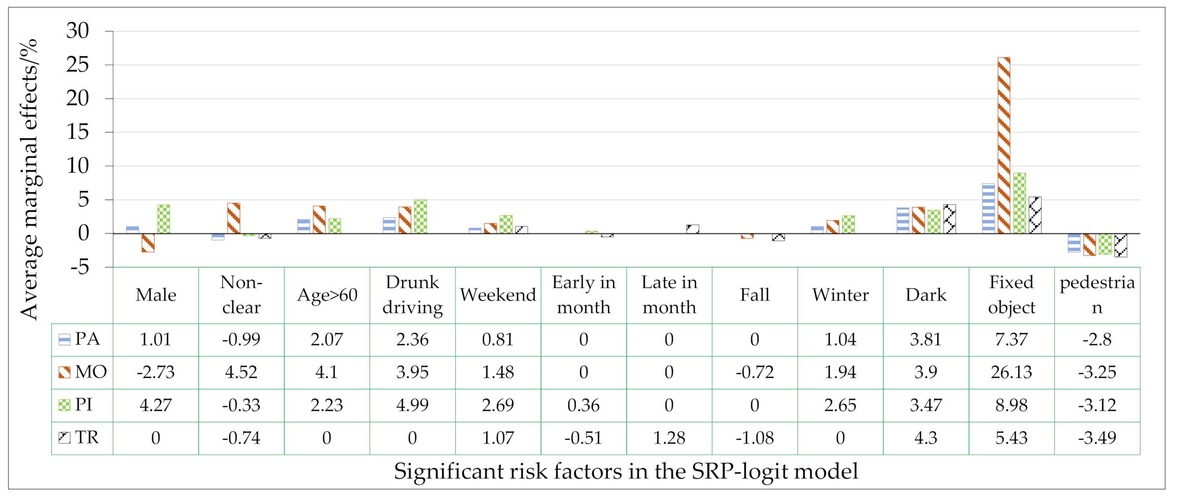
4.4. Average Marginal Effect

Model parameters can reflect the correlation between observed risk factors and crash severity (positive or negative correlation), but cannot measure how risk factors affect the probabilistic change in crash severity. Hence, the average marginal effect of the risk variables was calculated. Since the independent variables are transformed into binary indicator variables, the calculation rules are as follows:
E x i l Prob ( k ) = 1 I i = 1 I ( Prob ( k x i l = 1 ) - Prob ( k x i l = 0 ) ) ,  
where E x i l Prob ( k ) represents the average marginal effect to be calculated and can measure the probability change of crash severity when a variable is changed; x i l = 1 denotes the value of the l-th independent variable related to i-th crash is 1; Prob ( k x i l = 1 ) denotes the probability that crash severity is k when x i l = 1 ; similarly, Prob ( k x i l = 0 ) is the probability that crash severity is k when x i l = 0 . The term I denotes the total number of crashes.

5. Modeling Results and Discussion

5.1. Full Bayesian Estimation

A Full Bayesian (FB) approach has been widely recommended for determining the unknown parameters of a crash model [4,11]. The FB approach treats unknown parameters as random variables, and the corresponding distribution characteristics are defined by prior distribution. The core is to obtain posterior distribution by combining prior distribution and traditional likelihood function [43]. Hence, it is unavoidable to specify the prior distribution of (hyper-) parameters. In this study, a non-informative prior distribution was adopted due to lack of relevant knowledge. Specifically, a diffused normal distribution was specified for fixed parameters ( β l ,   β 0 ) and random parameters ( β i , l ,   β i , 0 ) , which can be expressed as:
β l ~ normal ( 0 τ ,   10 4 I τ ) β 0 ~ normal ( 0 τ ,   10 4 I τ ) ,   β i , l ~ normal ( 0 τ ,   10 4 I τ ) β i , 0 ~ normal ( 0 τ ,   10 4 I τ ) ,
where 0 τ denotes a zero vector of the form τ × 1 . I τ denotes a unit matrix of the form τ × τ .
Meanwhile, the prior distribution of precision parameters ( φ k , σ k , 0 2 , and σ u k 2 ) and σ s k 2 adopted the inverse gamma distribution and gamma distribution, respectively, which can be expressed as:
φ k ~ inverse   gamma ( 0.001 ,   0.001 ) σ k , 0 2 ~ inverse   gamma ( 0.001 ,   0.001 ) σ u k 2 ~ inverse   gamma ( 0.001 ,   0.001 ) σ s k 2 ~ gamma ( 1 + v w 2 ,   1 + n 2 ) ,
where 0.001 indicates the parameter of the inverse gamma distribution. v w represents the term contributed by each road segment, and the corresponding calculation rule is exhibited as follows [11]:
v w = w   w   δ w ,     w   s k w s k w - s k w ¯ .  
The computation of high-dimensional integrals in FB inference is difficult. Hence, a MCMC (Markov Chain Monte Carlo) simulation technique based on Metropolis-Hastings sampling was employed. The MCMC technique generates samples from posterior distribution and provides an efficient way to estimate the FB model. Considering the high complexity, 3 parallel MCMC simulation chains were created, and 30,000 iterations were maintained for each chain. The mean value of prior distribution was used as the initial value of model parameter and the real value was obtained by sufficient sampling simulation and removal of the burn-in period [11]. The first 15,000 iterations were discarded as the burn-in period because the posterior distribution achieves convergence after that; the other iterations were used for model estimation. Meanwhile, an intermittent sampling method was adopted to reduce sample correlation—that is, 1 of every 10 samples was reserved. The model estimation was implemented through the free software WinBUGS.
Several test measures were performed to determine the convergence of the MCMC chain and the relevance of the samples. First, the MCMC dynamic plot traces were visually checked. If parameter values lie within a region without strong periodicities, the conclusion of MCMC chain convergence can be drawn. Second, if all Brooks-Gelman–Rubin (BGR) statistics were lower than 1.2, the MCMC chains are considered to be convergent. The conclusion of model convergence can be obtained when both diagnostics are satisfied at the same time [64]. In addition, the autocorrelation plots (autocorrelation functions) were carefully examined to determine that the iterative chains were adequately close to independent and identically distributed (IID). If the autocorrelation value converged to zero soon after the iteration, the IID characteristic could meet the requirements.
To avoid the high correlation among risk factors, a Pearson’s correlation test was implemented to determine the appropriate independent variables. There was no obvious correlation between the two variables if the absolute value of Pearson’s correlation coefficient was less than 0.3 [55]. The correlation analysis showed high correlation between weather and road surface conditions and between crash time and lighting conditions, suggesting that these variables should be selected appropriately in the modeling process. The different covariates were accommodated separately in the model and the DIC values were compared to determine the superior independent variables. The Pearson’s correlation coefficients are shown in Figure 3. Only variables with no significant correlation were exhibited and used for subsequent modeling.

5.2. Model Comparison

The fitting performance indicators (DIC, pD, and D ¯ ) and classification accuracy (CA) value of the crash model across vehicle types are shown in Table 3; Table 4 exhibits the parameters of the MN-logit model and the RI-logit model, and Table 5 illustrates the coefficients of risk factors in the RP-logit model and the SRP-logit model. The interest response variable in this research is FS injuries; thus, the parameters that have a significant effect on FS injuries are given. Parameters are considered significant if the 90% Bayesian Credit Interval (90% BCI) does not contain zero. Otherwise, the parameters are found to be insignificant.
Among the crash models calibrated in this study, all parameters of the MN-logit model are fixed value (Table 4) because it cannot capture heterogeneity. In the RI-logit model, the coefficients of risk variable are fixed value, but the coefficient of intercept is random (Table 4). The heterogeneity in crash data is captured by the random variation of the intercept. Further, in the collision model established by the RP-logit function, both random coefficients and fixed coefficients are included (Table 5). Meanwhile, the number of random coefficients and fixed coefficients varies with vehicle types. In the SRP-logit model, three types of coefficients are accommodated, including the fixed coefficients, random coefficients, and coefficients of spatial variation (Table 5). Hence, the collision models established in this study accommodate the coefficients that can demonstrate the respective characteristics. The comparison of the fitting performance of these models is shown below.
From Table 3, some substantial differences in DIC and CA values across different logit approaches were found. First, passenger car crash function constructed by the MN-logit model had a higher DIC value (8859) than other models and the differences in DIC is greater than 5, 8827 for the RP-logit model, 8839 for the RI-logit model, and 8821 for the SRP-logit model. Similar phenomena were exhibited in the crash severity models of motorcycle, pickup, and truck. Meanwhile, the CA values associated with the MN-logit model were lower than other models, which remained stable across motor vehicle types. These findings indicated that the RI-logit model, the RP-logit model, and the SRP-logit model perform better than the MN-logit model and highlighted that the fitting performance and classification accuracy of the model can be improved by accommodating unobserved heterogeneity in crash severity analysis. Ye et al. [40] reached the same conclusion and gave a detailed discussion.
Second, among the three candidate heterogeneity models (RP-logit model, RI-logit model, SRP-logit model), the SRP-logit model was a superior approach for fitting rural SV crash severity, followed by the RP-logit model and the RI-logit model, and these findings were supported by all the vehicle types in this research.
More specifically, in the SRP-logit model, the RP-logit model, and the RI-logit model, the DIC values of passenger cars were 8821, 8827, and 8839, respectively, and of motorcycles were 8610, 8615, and 8631, respectively, and of trucks were 4184, 4205, and 4217, respectively. According to the statistical results, the DIC values of the three candidate models can be expressed in descending order, as follows—RI-logit model, RP-logit model, and SRP-logit model—and this finding remained stable across the three vehicle types. Furthermore, the differences in DIC were greater than 5. Hence, for passenger car, motorcycle, and truck crashes, the SRP-logit model exhibited the best fit performance, followed by the RP-logit model and the RI-logit model. Similar findings can be obtained by checking the CA values of such three vehicle types.
For pickup crashes, the DIC values of the SRP-logit model, RP-logit model, and RI-logit model were 2126, 2128, and 2137, respectively. It was found that the RP-logit model outperformed the RI-logit model. Note that the differences in DIC values between the SRP-logit model and the RP-logit model was less than 5; thus, DIC cannot be used for model diagnosis and CA values were adopted to determine the fitting performance. The values of CA1, CA2, CA3, and CAwhole in the SRP-logit model were 79.1%, 27.6%, 15.2%, and 75.8%, respectively, and in the RP-logit model were 73.6%, 20.8%, 8.9%, and 66.3%, respectively. It can be easily found that the prediction accuracy of the SRP-logit model outperforms that of the RP-logit model.
These findings suggested that simultaneously accounting for the unobserved heterogeneity across individual observations and spatial correlation among adjacent crashes could further improve the model fit. Similar findings were found by Yan et al. [65] and Zeng et al. [66] who pointed out that ignoring spatial correlation and unobserved heterogeneity in crash analysis will lead to biased estimates and incorrect inferences. Meanwhile, the significant spatial variations exhibit in Table 5 can further confirm the importance of accommodating spatial effects in rural SV crash severity analysis. In detail, the spatial variation ratios of no injury and slight injury associated with passenger cars were 0.712 and 0.543, respectively. In motorcycle crashes, the proportions of spatial variation in slight injury and FS injuries were statistically significant (the values were 0.691 and 0.850, respectively). The spatial variation of no injury in pickup collisions was significant (0.723) and of no injury and slight injury in truck crashes were significant (the values were 0.595 and 0.749, respectively).
Third, the numbers of effective parameters (pD) of passenger car crash functions established by the MN-logit model, RI-logit model, RP-logit model, and SRP-logit model were 62, 83, 115, and 138, respectively, highlighting a progressive increasing trend. This finding suggested that the SRP-logit model had higher complexity than other models because both the unstructured error term and the structured spatial error term were considered. Xu et al. [54] obtained similar conclusions and pointed out that capturing spatial effects through the first-order neighborhoods will generate a larger number of effective parameters and a better model fit compared to other definition methods. Interestingly, the greater number of effective parameters did not exhibit a negative effect for the fitting performance of the SRP-logit model. Because the posterior mean deviance ( D ¯ ) in the SRP-logit model has a greater degree of reduction; the posterior mean deviance of the MN-logit model, RI-logit model, RP-logit model, and SRP-logit model for passenger car crashes were 8797, 8756, 8712, and 8683, respectively. Similar conclusions can be drawn by checking the number of effective parameters and the posterior mean deviance of other vehicle types. This may be related to the fact that both the unobserved heterogeneity and the spatial correlation were contained in the SRP-logit model [54].
Finally, considering spatial correlation will result in some significant risk factors not being identical. According to the regression results of the SRP-logit model, there was no significant correlation between traffic control and FS injuries in passenger car crashes and between dark with street lighting and FS injuries in motorcycle crashes, but they became totally significant once spatial effect was not accommodated. This inconsistency may be due to model misspecification, including omission of spatially relevant variables [61].

5.3. Discussion

Compared with the MN-logit model, RP-logit model, and RI-logit model, the SRP-logit model has better fitting performance and classification accuracy. Hence, only the average marginal effects of significant risk factors in the SRP-logit model were calculated, and only the marginal effects associated with FS injuries were calculated.
Inspired by Lešnik et al. [67] and Mongus et al. [68], a histogram (Figure 4) was designed as a figure to represent the marginal effects, instead of a table. The aim is to interpret the model estimation results in a user-friendly way. Note that the marginal effects of risk factors that have no significant impact or have been artificially removed are denoted by zero. According to Figure 4, (1) for the same motor vehicle type, different risk factors have different impacts on FS injuries of rural SV crashes; (2) the effect of the same factor on FS injuries varies across motor vehicle types; and (3) among the various risk factors, collision with a fixed object has the greatest effect on FS injuries, which has remained stable across different vehicle types. A detailed discussion of risk factors based on the parameter estimation results and the average marginal effects of the SRP-logit model is provided below.
There is significant correlation between male driver and FS injuries in rural SV crashes. However, the sign of correlation (positive or negative correlation) varies with motor vehicle type. Male drivers are significantly and positively associated with FS injuries in passenger car and pickup crashes, with average marginal effects of 1.01% and 4.27%, respectively. A similar finding was obtained by Lawrence et al. [69], who noted that male drivers were 2.18 times more likely to result in serious passenger car crashes than females. However, there is a significant negative correlation between male drivers and FS injuries in rural motorcycle SV crashes, with average marginal effects of −2.73%. Vajari et al. [37] reached a similar conclusion by analyzing the severity of motorcycle crashes at Australian intersections. These findings are of interest to comprehensively elucidate the variable effects of male driver on rural SV crash severity and validate the necessity of regression analysis based on different vehicle types. Further, for all vehicle types, the parameters of male driver exhibit random effects obeying a normal distribution. This finding is supported by many research studies [16,21] and highlighted that capturing unobserved heterogeneity is indispensable during the crash severity modeling process.
For motorcycle crashes, non-clear weather is significantly and positively associated with FS injuries in rural SV crashes (marginal effect 4.52%), which is consistent with previous research [37], because rural China has poor traffic conditions, such as waterlogged and narrower roads. In addition, motorcycles do not have satisfactory stability because of two tires [70]. Hence, serious motorcycle crashes occur frequently in non-clear weather. However, there is a significant negative correlation between non-clear weather and FS injuries for other vehicle types. The probability of serious rural SV crashes caused by passenger car, pickup, and truck under non-clear weather conditions is reduced by 0.99%, 0.33%, and 0.74% respectively. Shaheed et al. [71] and Cerwick et al. [72] reached the same conclusion and pointed out that this phenomenon was caused by cautious driving under unsatisfactory weather conditions.
For passenger car, motorcycle, and pickup crashes, the relationship between older adult driver (age > 60) and FS injuries is significant at the 95% BCI, and the probability of serious injury caused by older adult drivers increased by 2.07%, 4.10%, and 2.23%, respectively, compared to mid-age drivers (30–60). The same conclusion was reached by Xie et al. [15] and Abdel-Aty [73] and noted that the physical capabilities of older drivers are not satisfactory, as they require more reaction time in case of an emergency, which result in a greater susceptibility to serious crashes [74]. However, this variable becomes totally insignificant once truck crashes are accommodated. Cai et al. [59] obtained a similar conclusion by analyzing rural SV crashes in China and believed that more driving experience may be a dominant factor in determining crash severity. Hence, government departments may consider providing regular training and driving skills tests for older adults, with the aim of improving their traffic safety performance.
The impact of drunk driving on traffic safety cannot be ignored. In passenger car, motorcycle, and pickup crashes, drunk driving will result in a significant increase in the probability of severe rural SV crashes (marginal effects 2.36%, 3.95%, and 4.99%, respectively). This finding is confirmed in the existing literature [75,76], which points out that if a driver is under the influence of alcohol, it is difficult to maintain a satisfactory driving status and is more likely to be involved in serious rural SV crashes. These findings demonstrate the detrimental effects of drunk driving on rural traffic safety to policymakers and the general public. Furthermore, traffic management and road infrastructure in rural China are inadequate, which further increases the probability of serious collisions. The percentage of drunk driving in the whole dataset is as high as 15.33%; hence, the management of drunk driving should be strengthened. Note that drunk driving in the model of truck crashes was artificially deleted because it had only 33 observations (0.6%). The statistical results show that truck drivers have superior safety awareness compared to other motor vehicle types; a similar finding was pointed out by Cerwick et al. [72]. In addition, the parameter of drunk driving in the model of rural motorcycle SV crashes follows a normal distribution with a mean of 0.163 and a standard deviation of 1.408. However, there is no heterogeneity for this variable in other vehicle types. Hence, by establishing rural SV crash models under different vehicle types, the source of heterogeneity of risk factors in the whole dataset can be clarified.
The impact of the weekend on the severity of rural SV crashes is significant, which remained stable across different vehicle types. Weekend driving resulted in a 0.81%, 1.48%, 2.69%, and 1.07% increase in the probability of FS injuries in passenger car, motorcycle, pickup, and truck crashes, respectively. This is generally consistent with the previous studies. For example, Vajari et al. [37] and Cerwick et al. [72] analyzed motorcycle crashes and truck crashes, respectively, and both suggested that the probability of a serious crash was significantly higher on weekends than on weekdays. These findings underscore the importance of educating drivers to remain vigilant after long off-duty hours, such as on weekends, and provide theoretical references for formulating scientific management measures. For example, traffic management in weekends should be strengthened.
There is a significant correlation between early in the month and FS injuries in pickup and truck crashes. Interestingly, this variable is positively correlated with FS injuries in rural pickup SV crashes (marginal effect 0.36%) and is negatively correlated with FS injuries in rural truck SV crashes (marginal effect −0.51%). In addition, late in the month has a significant positive influence on FS injuries in rural truck SV crashes (marginal effect 1.28%) but no significant impact was found on other vehicle types. Based on in-depth understanding of the literature, few research studies considered the impact of this variable on crash severity. Hence, these novel and interesting discoveries can further enrich existing research and can be used to effectively assign law enforcement duties—for example, increased supervision of pickups in the first 10-day period of a month and of trucks in the last 10-day period of a month in rural areas.
According to the regression results, the probability of FS injuries in rural SV collisions varies with the seasons. More specifically, motorcycle and truck crashes in autumn are less likely to result in serious injuries (marginal effects −0.72% and −1.08%, respectively). This finding can be proved by existing research; for example, it was found that the probability of severe truck crashes and severe motorcycle crashes in autumn reduced by 0.07% [72] and 0.03% [77], respectively. The coefficient of autumn is not statistically significant in other motor vehicle types. Further, passenger car, motorcycle, and pickup are more likely to be involved in severe rural SV crashes during the winter, with corresponding probabilities increasing by 1.04%, 1.94%, and 2.65%, respectively. However, there is no significant correlation between FS injuries and winter in rural truck SV crashes. These findings are indispensable and demonstrate the effectiveness of modeling rural SV crashes based on motor vehicle type to reveal the variable effects of risk factors. Meanwhile, the research results indicate that the traffic safety performance of rural roadways in winter is unsatisfactory and underscore the importance of traffic management during winter.
A significant positive correlation between dark (without street lighting) condition and FS injuries in rural SV crashes was determined, which is supported by all vehicle types. The probability of FS injuries in dark (without street lighting) conditions increased by 3.81%, 3.90%, 3.47%, and 4.30% for passenger car, motorcycle, pickup, and truck crashes, respectively. A largely consistent finding can be found in [69], which represents this variable by complete darkness. Furthermore, there is no significant correlation between street lighting and FS injuries, which is supported by all vehicle types considered in this research. This can be confirmed by previous research [78]. These findings are valuable to improve the safety performance in rural areas. For traffic managers, the installation of streetlamps on rural roadways is indispensable; for ordinary drivers, cautious driving should be maintained under dark (without street lighting) condition.
Almost all researches concluded that there is a significant positive correlation between collision with fixed object and severe rural SV crashes [21,76,79]; the same conclusion is drawn in this study. By modeling injury severity of rural SV crashes across different vehicle types, the destabilizing effects of risk variables can be revealed. In passenger car, motorcycle, pickup, and truck crashes, the probability of FS injuries caused by collision with fixed object increased by 7.37%, 26.13%, 8.98%, and 5.43%, respectively. Among them, the highest probability is maintained by motorcycle due to it not providing adequate protection. Further, rural SV collisions between motorcycle and fixed object could easily result in rollovers, which will cause riders to collide violently with hard objects such as the road surface and significantly increase the likelihood of serious injury. It has been widely reported that the principal cause of fatality among motorcyclists is head injury [80]. Wearing a helmet can effectively protect motorcyclists from head injuries [75]; however, 60.1% of riders in motorcycle crashes do not use helmets. Hence, it is necessary to strengthen the management of riders. In addition, roadside fixtures such as stone pillars in traffic infrastructure, which can effectively guide traffic operations, are a potential traffic safety hazard due to the collision energy that cannot be absorbed by the fixed object. Therefore, the use of roadside facilities with a buffering function, such as plastic guardrails, may be a superior choice.
There is a significant negative correlation between collision with pedestrians and FS injuries in rural SV crashes, which remained stable across different vehicle types. For passenger car, motorcycle, pickup, and truck crashes, the marginal effects are −2.8%, −3.25%, −3.12%, and −3.49%, respectively. This finding is reasonable and can be confirmed in existing studies. For example, SV crashes under foggy weather and clear weather were analyzed and the probabilities of serious driver injury resulting from collision with pedestrians were reduced by 8.5% and 13.3%, respectively [51]. Generally, pedestrians are vulnerable compared to motor vehicles, and collisions with pedestrians are not expected to result in serious injury to motorists. On the contrary, there is a high probability to take the life of pedestrians [25].

5.4. Model Transferability

The goodness-of-fit and prediction accuracy of the SRP-logit model are optimal compared to other models developed in this study; hence, the transferability of the SRP-logit model across different vehicle types was investigated. The calculation results of TI values are shown in Table 6.
The diagonals in Table 6 have a value of 1, as they represent the respective local conditions. In addition, most of the transfer indices on both sides of the diagonal are negative, suggesting that the local constant-only model outperforms the transfer model. The exception is that the transfer indices between passenger car and pickup show a positive relationship. This may be related to the similar structure of the passenger car and pickup. Nonetheless, the transferability indices indicate that the SPFs of passenger car and pickup cannot be transferred directly in traffic safety analysis (the transfer indices are 0.417 and 0.329, respectively, which are much smaller than 1) [62]. Therefore, a separate SPF for each vehicle type is needed in rural safety diagnosis.

5.5. Recommendations

The usefulness and implications of this research mainly includes two parts:
(1) the SRP-logit model was proposed to comprehensively accommodate the unobserved heterogeneity and the spatial correlation and to improve the fitting performance of the statistical model for rural SV crashes. This finding promotes the development of the statistical theory in traffic safety analysis and can provide a satisfactory model framework for traffic safety professionals.
(2) Based on different types of motor vehicles, rural SV crash severity models were established to identify factors that have a significant impact on FS injuries. According to the regression results and previous practical experience, targeted measures can be implemented to remind drivers and improve traffic safety performance in rural areas. The details are shown as follows.
First, there is a significant correlation between driving behavior and severe collisions. Some risky driving behaviors, such as drunk driving, fatigue, and speeding, can affect the probability and severity of crashes in different ways. Legal measures can effectively reduce risky driving behaviors. Installing electronic police and speed limit signs on rural roadways can effectively remind drivers and improve rural traffic safety. Safety education for drivers is also essential.
Second, the impact of roadside fixtures on rural traffic safety cannot be ignored. Traffic managers should consider installing a soft protective cover on the surface of roadside infrastructure to absorb collision energy. In addition, streetlights should be installed along rural roads because they can improve traffic safety in rural areas by providing a good view.
Finally, motorcycles cannot provide adequate protection for drivers. Therefore, more education and encouragement for riders should be implemented to improve their traffic safety awareness. Some legal measures should be formulated to increase the percentage of helmet wearers.

6. Conclusions

This study investigated the influence of risk factors on the severity of rural SV crashes across different vehicle types (passenger car, motorcycle, pickup, and truck). To accommodate the cross-road segments heterogeneity, a novel SRP-logit model accounting for both unobserved heterogeneity and spatial correlation under a Bayesian framework was proposed.
Five years of SV crash data in a rural area were used to calibrate the proposed model. Three candidate logit approaches—MN-logit model, RP-logit model, and RI-logit model—were established and compared with the SRP-logit model. The model comparison shows that the SRP-logit model exhibits the best fit performance, followed by the RP-logit model, RI-logit model, and MN-logit model. This finding suggests that it is necessary to capture the unobserved heterogeneity in the rural SV crash analysis, which can initially improve the fitting performance of the crash model. The model fit can be further improved by simultaneously accounting for the unobserved heterogeneity across individual observations and the spatial correlation among adjacent crashes.
Several risk factors are significantly associated with FS injuries in rural SV crashes, and the impacts of risk factors on crash severity varies across different vehicle types. Specifically, in passenger car and pickup crashes, there is a positive association between male drivers and FS injuries; however, a significant negative correlation is shown in motorcycle collisions. Non-clear weather maintains a significant negative effect on FS injuries in passenger car, pickup, and truck crashes and a significant positive effect on FS injuries in motorcycle crashes. Similar findings can be found in the coefficients of season and early in month.
In addition, there is a significant positive correlation between weekend, dark (without street lighting) conditions and collision with fixed object and FS injuries. Collisions with pedestrians are not expected to cause serious injury to drivers. These findings are shared across different vehicle types.

7. Limitations of This Study

There are some limitations of the current study, which will be resolved in future research:
(1)
Although many potential risk factors are considered in this research, some real-time factors that may also have effects on the severity of rural SV crashes are unavailable in police collision reports, such as real-time traffic volume and vehicle speed. It is expected that the fitting performance of the SRP-logit model can be improved if these variables are accommodated. Transportation facilities are not perfect in rural areas of China, which leads to a lack of traffic data; hence, some data collection equipment should be set up in specific rural locations for further research.
(2)
The insignificant variables were removed from the final model, which may introduce omitted variable bias. We will consider optimizing the statistical modeling framework to propose more reasonable judgments.
(3)
The research results showed that the transferability of the crash severity model between different vehicle types is unsatisfactory. This may be due to substantial differences between different motor vehicle types. In the future, more advanced methods need to be explored to improve model transferability. Further, due to the differences in cultural backgrounds and driving habits among different countries, the applicability of statistical methods proposed in this research needs to be explored.

Author Contributions

Study concept and design: F.W., Z.C., Y.G. and Z.W.; data collection: F.W., X.W. and X.L.; data analysis and interpretation of results: Z.W. and Z.C.; draft manuscript preparation: F.W., Y.G. and Z.C.; manuscript revision: Y.G., F.W. and Z.W. All authors have read and agreed to the published version of the manuscript.

Funding

This research was jointly supported by (1) the National Natural Science Foundation of China (Grant No. 71901134, 51905320 and 71871057); (2) the National Science Foundation for Distinguished Young Scholars (Grant No. 51925801); and (3) the Natural Science Foundation of Shandong (Grant No. ZR2018BF024).

Institutional Review Board Statement

Not applicable.

Informed Consent Statement

Not applicable.

Data Availability Statement

Not applicable.

Acknowledgments

The authors are thankful for the support of the Shandong Department of Transportation (SDOT), the Zibo Department of Transportation (ZDOT), and the Center for Accident Research in Zibo (CARZ).

Conflicts of Interest

The authors declare that they have no known competing financial interests or personal relationships that could have appeared to influence the work reported in this paper.

References

  1. Traffic Management Bureau of Ministry of Public Security of China. Statistics Annals of Road Traffic Accident of People’s Republic of China (2017); Traffic Management Science Institute of Ministry of Public Security: Wuxi, China, 2018. [Google Scholar]
  2. Zheng, L.; Sayed, T.; Mannering, F. Modeling traffic conflicts for use in road safety analysis: A review of analytic methods and future directions. Anal. Methods Accid. Res. 2020, 29, 100142. [Google Scholar] [CrossRef]
  3. Theofilatos, A.; Yannis, G. A review of the effect of traffic and weather characteristics on road safety. Accid. Anal. Prev. 2014, 72, 244–256. [Google Scholar] [CrossRef] [PubMed]
  4. Guo, Y.; Sayed, T.; Essa, M. Real-time conflict-based Bayesian Tobit models for safety evaluation of signalized intersections. Accid. Anal. Prev. 2020, 144, 105660. [Google Scholar] [CrossRef] [PubMed]
  5. Xu, C.; Liu, P.; Wang, W.; Zhang, Y. Real-time identification of traffic conditions prone to injury and non-injury crashes on freeways using genetic programming. J. Adv. Transp. 2016, 50, 701–716. [Google Scholar] [CrossRef] [Green Version]
  6. Xu, C.; Liu, P.; Wang, W.; Li, Z. Evaluation of the impacts of traffic states on crash risks on freeways. Accid. Anal. Prev. 2012, 47, 162–171. [Google Scholar] [CrossRef]
  7. Li, Z.; Wang, W.; Liu, P.; Bigham, J.M.; Ragland, D.R. Using geographically weighted Poisson regression for county-level crash modeling in California. Saf. Sci. 2013, 58, 89–98. [Google Scholar] [CrossRef]
  8. Guo, Y.; Sayed, T.; Zheng, L. A hierarchical Bayesian peak over threshold approach for conflict-based before-after safety evaluation of leading pedestrian intervals. Accid. Anal. Prev. 2020, 147, 105772. [Google Scholar] [CrossRef]
  9. Yu, H.; Li, Z.; Zhang, G.; Liu, P. A latent class approach for driver injury severity analysis in highway single-vehicle crash considering unobserved heterogeneity and temporal influence. Anal. Methods Accid. Res. 2019, 24, 100110. [Google Scholar] [CrossRef]
  10. Xu, C.; Tarko, A.P.; Wang, W.; Liu, P. Predicting crash likelihood and severity on freeways with real-time loop detector data. Accid. Anal. Prev. 2013, 57, 30–39. [Google Scholar] [CrossRef]
  11. Guo, Y.; Osama, A.; Sayed, T. A cross-comparison of different techniques for modeling macro level cyclist crashes. Accid. Anal. Prev. 2018, 113, 38–46. [Google Scholar] [CrossRef]
  12. Wen, H.; Xue, G. Injury severity analysis of familiar drivers and unfamiliar drivers in single-vehicle crashes on the mountainous highways. Accid. Anal. Prev. 2020, 144, 105667. [Google Scholar] [CrossRef]
  13. Islam, S.; Jones, S.; Dye, D.L. Comprehensive analysis of single- and multi-vehicle large truck at fault crashes on rural and urban roadways in Alabama. Accid. Anal. Prev. 2014, 67, 148–158. [Google Scholar] [CrossRef] [PubMed]
  14. Chen, C.; Xie, Y. The impacts of multiple rest break periods on commercial truck driver’s crash risk. J. Saf. Res. 2014, 48, 87–93. [Google Scholar] [CrossRef]
  15. Xie, Y.; Zhao, K.; Huynh, N. Analysis of driver injury severity in rural single-vehicle crashes. Accid. Anal. Prev. 2012, 47, 36–44. [Google Scholar] [CrossRef]
  16. Wu, Q.; Zhang, G.; Zhu, X.; Liu, X.C.; Tarefder, R. Analysis of driver injury severity in single-vehicle crashes on rural and urban roadways. Accid. Anal. Prev. 2016, 94, 35–45. [Google Scholar] [CrossRef]
  17. Duddu, V.R.; Pulugurtha, S.S.; Kukkapalli, V.M. Variable categories influencing single-vehicle run-off-road crashes and their severity. Transp. Eng. 2020, 2, 100038. [Google Scholar] [CrossRef]
  18. Gong, L.; Fan, W. Modeling single-vehicle run-off-road crash severity in rural areas: Accounting for unobserved heterogeneity and age difference. Accid. Anal. Prev. 2017, 101, 124–134. [Google Scholar] [CrossRef] [PubMed]
  19. Haq, M.T.; Zlatkovic, M.; Ksaibati, K. Investigating occupant injury severity of truck-involved crashes based on vehicle types on a mountainous freeway: A hierarchical Bayesian random intercept approach. Accid. Anal. Prev. 2020, 144, 105654. [Google Scholar] [CrossRef] [PubMed]
  20. Yu, M.; Ma, C.; Shen, J. Temporal stability of driver injury severity in single-vehicle roadway departure crashes: A random thresholds random parameters hierarchical ordered probit approach. Anal. Methods Accid. Res. 2020, 29, 100144. [Google Scholar] [CrossRef]
  21. Yu, H.; Yuan, R.; Li, Z.; Zhang, G.; Ma, D.T. Identifying heterogeneous factors for driver injury severity variations in snow-related rural single-vehicle crashes. Accid. Anal. Prev. 2020, 144, 105587. [Google Scholar] [CrossRef] [PubMed]
  22. Wei, F.; Cai, Z.; Guo, Y.; Liu, P.; Wang, Z.; Li, Z. Analysis of roadside accident severity on rural and urban roadways. Intell. Autom. Soft Comput. 2021, 28, 753–767. [Google Scholar] [CrossRef]
  23. Bhowmik, T.; Yasmin, S.; Eluru, N. Do we need multivariate modeling approaches to model crash frequency by crash types? A panel mixed approach to modeling crash frequency by crash types. Anal. Methods Accid. Res. 2019, 24, 100107. [Google Scholar] [CrossRef]
  24. Wu, Q.; Chen, F.; Zhang, G.; Liu, X.C.; Wang, H.; Bogus, S.M. Mixed logit model-based driver injury severity investigations in single- and multi-vehicle crashes on rural two-lane highways. Accid. Anal. Prev. 2014, 72, 105–115. [Google Scholar] [CrossRef]
  25. Zhai, X.; Huang, H.; Sze, N.N.; Song, Z.; Hon, K.K. Diagnostic analysis of the effects of weather condition on pedestrian crash severity. Accid. Anal. Prev. 2018, 122, 318–324. [Google Scholar] [CrossRef] [PubMed]
  26. Li, Z.; Liu, P.; Wang, W.; Xu, C. Using support vector machine models for crash injury severity analysis. Accid. Anal. Prev. 2012, 45, 478–486. [Google Scholar] [CrossRef]
  27. Zhang, J.; Li, Z.; Pu, Z.; Xu, C. Comparing prediction performance for crash injury severity among various machine learning and statistical methods. IEEE Access 2019, 6, 60079–60087. [Google Scholar] [CrossRef]
  28. Rezapour, M.; Moomen, M.; Ksaibati, K. Ordered logistic models of influencing factors on crash injury severity of single and multiple-vehicle downgrade crashes: A case study in Wyoming. J. Saf. Res. 2019, 68, 107–118. [Google Scholar] [CrossRef] [PubMed]
  29. Rahman, M.A.; Sun, X.; Das, S.; Khanal, S. Exploring the influential factors of roadway departure crashes on rural two-lane highways with logit model and association rules mining. Int. J. Transp. Sci. Technol. 2021, 10, 167–183. [Google Scholar] [CrossRef]
  30. Li, Z.; Wu, Q.; Ci, Y.; Chen, C.; Chen, X.; Zhang, G. Using latent class analysis and mixed logit model to explore risk factors on driver injury severity in single-vehicle crashes. Accid. Anal. Prev. 2019, 129, 230–240. [Google Scholar] [CrossRef]
  31. Wei, F.; Guo, Y.; Liu, P.; Cai, Z.; Li, Q.; Chen, L. Modeling Car-Following behaviour of turning movements at intersections with consideration of turning radius. J. Adv. Transp. 2020, 2020, 8884797. [Google Scholar] [CrossRef]
  32. Li, Z.; Li, Y.; Liu, P.; Wang, W.; Xu, C. Development of a variable speed limit strategy to reduce secondary collision risks during inclement weathers. Accid. Anal. Prev. 2014, 72, 134–145. [Google Scholar] [CrossRef] [PubMed]
  33. Li, Z.; Xu, C.; Li, D.; Liu, P.; Wang, W. Comparing the effects of ramp metering and variable speed limit on reducing travel time and crash risk at bottlenecks. IET Intell. Transp. Syst. 2017, 12, 120–126. [Google Scholar] [CrossRef]
  34. Li, Z.; Liu, P.; Wang, W.; Xu, C. Development of a control strategy of variable speed limits to reduce rear-end collision risks near freeway recurrent bottlenecks. IEEE Trans. Intell. Transp. Syst. 2014, 15, 866–877. [Google Scholar] [CrossRef]
  35. Chen, Y.; Luo, R.; Yang, H.; King, M.; Shi, Q. Applying latent class analysis to investigate rural highway single-vehicle fatal crashes in China. Accid. Anal. Prev. 2020, 148, 105840. [Google Scholar] [CrossRef]
  36. Park, S.; Jovanis, P. Hours of service and truck crash risk: Findings from three national U.S. carriers during 2004. Transp. Res. Rec. 2010, 2194, 3–10. [Google Scholar] [CrossRef]
  37. Vajari, M.A.; Aghabayk, K.; Sadeghian, M.; Shiwakoti, N. A multinomial logit model of motorcycle crash severity at Australian intersections. J. Saf. Res. 2020, 73, 17–24. [Google Scholar] [CrossRef] [PubMed]
  38. Chen, Z.; Fan, W.D. A multinomial logit model of pedestrian-vehicle crash severity in North Carolina. Int. J. Transp. Sci. Technol. 2019, 8, 43–52. [Google Scholar] [CrossRef]
  39. Milton, J.C.; Shankar, V.N.; Mannering, F.L. Highway accident severities and the mixed logit model: An exploratory empirical analysis. Accid. Anal. Prev. 2008, 40, 260–266. [Google Scholar] [CrossRef] [PubMed]
  40. Ye, F.; Lord, D. Comparing three commonly used crash severity models on sample size requirements: Multinomial logit, ordered probit and mixed logit models. Anal. Methods Accid. Res. 2014, 1, 72–85. [Google Scholar] [CrossRef] [Green Version]
  41. Xu, C.; Wang, W.; Liu, P. Real-time identification of crash-prone traffic conditions under different weather on freeways. J. Saf. Res. 2013, 46, 135–144. [Google Scholar] [CrossRef] [PubMed]
  42. Chen, C.; Zhang, G.; Tian, Z.; Bogus, S.M.; Yang, Y. Hierarchical Bayesian random intercept model-based cross-level interaction decomposition for truck driver injury severity investigations. Accid. Anal. Prev. 2015, 85, 186–198. [Google Scholar] [CrossRef] [PubMed]
  43. Zeng, Q.; Gu, W.; Zhang, X.; Wen, H.; Lee, J.; Hao, W. Analyzing freeway crash severity using a Bayesian spatial generalized ordered logit model with conditional autoregressive priors. Accid. Anal. Prev. 2019, 127, 87–95. [Google Scholar] [CrossRef]
  44. Aguero-Valverde, J.; Jovanis, P. Analysis of road crash frequency with spatial models. Transp. Res. Rec. 2008, 2061, 55–63. [Google Scholar] [CrossRef]
  45. Klassen, J.; El-Basyouny, K.; Islam, M.T. Analyzing the severity of bicycle-motor vehicle collision using spatial mixed logit models: A city of Edmonton case study. Saf. Sci. 2014, 62, 295–304. [Google Scholar] [CrossRef]
  46. Lee, J.; Yasmin, S.; Eluru, N.; Abdel-Aty, M.; Cai, Q. Analysis of crash proportion by vehicle type at traffic analysis zone level: A mixed fractional split multinomial logit modeling approach with spatial effects. Accid. Anal. Prev. 2018, 111, 12–22. [Google Scholar] [CrossRef]
  47. Xu, X.; Luo, X.; Ma, C.; Xiao, D. Spatial-temporal analysis of pedestrian injury severity with geographically and temporally weighted regression model in Hong Kong. Transp. Res. Part F Traffic Psychol. Behav. 2020, 69, 286–300. [Google Scholar] [CrossRef]
  48. Guo, Y.; Li, Z.; Liu, P.; Wu, Y. Modeling correlation and heterogeneity in crash rates by collision types using full Bayesian random parameters multivariate Tobit model. Accid. Anal. Prev. 2019, 128, 164–174. [Google Scholar] [CrossRef] [PubMed]
  49. Cai, Q.; Abdel-Aty, M.; Lee, J.; Wang, L.; Wang, X. Developing a grouped random parameters multivariate spatial model to explore zonal effects for segment and intersection crash modeling. Anal. Methods Accid. Res. 2018, 19, 1–15. [Google Scholar] [CrossRef]
  50. Huang, H.; Chang, F.; Zhou, H.; Lee, J. Modeling unobserved heterogeneity for zonal crash frequencies: A Bayesian multivariate random-parameters model with mixture components for spatially correlated data. Anal. Methods Accid. Res. 2019, 24, 100105. [Google Scholar] [CrossRef]
  51. Wei, F.; Cai, Z.; Liu, P.; Guo, Y.; Li, X.; Li, Q. Exploring driver injury severity in single-vehicle crashes under foggy weather and clear weather. J. Adv. Transp. 2021, 2021, 9939800. [Google Scholar] [CrossRef]
  52. Zhou, H.; Yuan, C.; Dong, N.; Wong, S.C.; Xu, P. Severity of passenger injuries on public buses: A comparative analysis of collision injuries and non-collision injuries. J. Saf. Res. 2020, 74, 55–69. [Google Scholar] [CrossRef] [PubMed]
  53. Ahmed, M.M.; Franke, R.; Ksaibati, K.; Shinstine, D.S. Effects of truck traffic on crash injury severity on rural highways in Wyoming using Bayesian binary logit models. Accid. Anal. Prev. 2018, 117, 106–113. [Google Scholar] [CrossRef] [PubMed]
  54. Xu, X.; Xie, S.; Wong, S.C.; Xu, P.; Huang, H.; Pei, X. Severity of pedestrian injuries due to traffic crashes at signalized intersections in Hong Kong: A Bayesian spatial logit model. J. Adv. Transp. 2017, 50, 2015–2028. [Google Scholar] [CrossRef]
  55. Zhang, X.; Wen, H.; Yamamoto, T.; Zeng, Q. Investigating hazardous factors affecting freeway crash injury severity with real-time weather data: Using a Bayesian multinomial logit model with conditional autoregressive priors. J. Saf. Res. 2021, 76, 248–255. [Google Scholar] [CrossRef] [PubMed]
  56. Shankar, V.; Mannering, F. An exploratory multinomial logit analysis of single-vehicle motorcycle accident severity. J. Saf. Res. 1996, 27, 183–194. [Google Scholar] [CrossRef]
  57. Xu, C.; Wang, W.; Liu, P. A genetic programming model for real-time crash prediction on freeways. IEEE Trans. Intell. Transp. 2012, 14, 574–586. [Google Scholar] [CrossRef]
  58. El-Basyouny, K.; Sayed, T. Urban arterial accident prediction models with spatial effects. Transp. Res. Rec. 2009, 2102, 27–33. [Google Scholar] [CrossRef]
  59. Cai, Z.; Wei, F.; Wang, Z.; Guo, Y.; Chen, L.; Li, X. Modeling of Low Visibility-Related Rural Single-Vehicle Crashes Considering Unobserved Heterogeneity and Spatial Correlation. Sustainability 2021, 13, 7438. [Google Scholar] [CrossRef]
  60. Karim, M.; Wahba, M.; Sayed, T. Spatial effects on zone-level collision prediction models. Transp. Res. Rec. 2013, 2398, 50–59. [Google Scholar] [CrossRef]
  61. Munira, S.; Sener, I.N.; Dai, B. A Bayesian spatial Poisson-lognormal model to examine pedestrian crash severity at signalized intersections. Accid. Anal. Prev. 2020, 144, 105679. [Google Scholar] [CrossRef]
  62. Farid, A.; Abdel-Aty, M.; Lee, J.; Eluru, N.; Wang, J.H. Exploring the transferability of safety performance functions. Accid. Anal. Prev. 2016, 94, 143–152. [Google Scholar] [CrossRef] [PubMed]
  63. Spiegelhalter, D.J.; Best, N.G.; Carlin, B.P.; Linde, A.V.D. Bayesian measures of model complexity and fit. J. R. Stat. Soc. 2002, 64, 583–639. [Google Scholar] [CrossRef] [Green Version]
  64. Guo, Y.; Li, Z.; Liu, P.; Wu, Y. Exploring risk factors with crashes by collision type at freeway diverge areas: Accounting for unobserved heterogeneity. IEEE Access 2019, 7, 11809–11819. [Google Scholar] [CrossRef]
  65. Yan, X.; He, J.; Zhang, C.; Liu, Z.; Wang, C.; Qiao, B. Spatiotemporal instability analysis considering unobserved heterogeneity of crash-injury severities in adverse weather. Anal. Methods Accid. Res. 2021, 32, 100182. [Google Scholar] [CrossRef]
  66. Zeng, Q.; Wen, H.; Huang, H.; Abdel-Aty, M. A Bayesian spatial random parameters Tobit model for analyzing crash rates on roadway segments. Accid. Anal. Prev. 2017, 100, 37–43. [Google Scholar] [CrossRef]
  67. Lešnik, U.; Mongus, D.; Jesenko, D. Predictive analytics of PM10 concentration levels using detailed traffic data. Transp. Res. Part D Transp. Environ. 2019, 67, 131–141. [Google Scholar] [CrossRef]
  68. Mongus, D.; Vilhar, U.; Skudnik, M.; Žalik, B.; Jesenko, D. Predictive analytics of tree growth based on complex networks of tree competition. For. Ecol. Manag. 2018, 425, 164–176. [Google Scholar] [CrossRef]
  69. Lawrence, T.L.; Norton, R.; Woodward, M.; Connor, J.; Ameratunga, S. Passenger carriage and car crash injury: A comparison between younger and older drivers. Accid. Anal. Prev. 2003, 35, 861–867. [Google Scholar] [CrossRef]
  70. Salum, J.; Kitali, A.E.; Bwire, H.; Sando, T. Severity of motorcycle crashes in Dares Salaam, Tanzania. Traffic Inj. Prev. 2019, 20, 189–195. [Google Scholar] [CrossRef]
  71. Shaheed, M.S.; Gkritza, K.; Carriquiry, A.L.; Hallmark, S.L. Analysis of occupant injury severity in winter weather crashes: A fully Bayesian multivariate approach. Anal. Methods Accid. Res. 2016, 11, 33–47. [Google Scholar] [CrossRef]
  72. Cerwick, D.M.; Gkritza, K.; Shaheed, M.S.; Hans, Z. A comparison of the mixed logit and latent class methods for crash severity analysis. Anal. Methods Accid. Res. 2014, 3, 11–27. [Google Scholar] [CrossRef]
  73. Abdel-Aty, M. Analysis of driver injury severity levels at multiple locations using ordered probit models. J. Saf. Res. 2003, 34, 597–603. [Google Scholar] [CrossRef] [PubMed]
  74. Hamido, S.; Hamamoto, R.; Gu, X.; Itoh, K. Factors influencing occupational truck driver safety in ageing society. Accid. Anal. Prev. 2021, 150, 105922. [Google Scholar] [CrossRef]
  75. Chang, F.; Xu, P.; Zhou, H.; Chan, A.H.S.; Huang, H. Investigating injury severities of motorcycle riders: A two-step method integrating latent class cluster analysis and random parameters logit model. Accid. Anal. Prev. 2019, 131, 316–326. [Google Scholar] [CrossRef]
  76. Li, Z.; Ci, Y.; Chen, C.; Zhang, G.; Wu, Q.; Qian, Z.; Prevedouros, P.D.; Ma, D.T. Investigation of driver injury severities in rural single-vehicle crashes under rain conditions using mixed logit and latent class models. Accid. Anal. Prev. 2019, 124, 219–229. [Google Scholar] [CrossRef] [PubMed]
  77. Waseem, M.; Ahmed, A.; Saeed, T.U. Factors affecting motorcyclists’ injury severities: An empirical assessment using random parameters logit model with heterogeneity in means and variances. Accid. Anal. Prev. 2019, 123, 12–19. [Google Scholar] [CrossRef] [PubMed]
  78. Islam, M.B.; Hernandez, S. Modeling injury outcomes of crashes involving heavy vehicles on Texas highways. Transp. Res. Rec. 2013, 2388, 28–36. [Google Scholar] [CrossRef] [Green Version]
  79. Li, Z.; Chen, C.; Wu, Q.; Zhang, G.; Liu, C.; Prevedouros, P.D.; Ma, D.T. Exploring driver injury severity patterns and causes in low visibility related single-vehicle crashes using a finite mixture random parameters model. Anal. Methods Accid. Res. 2018, 20, 1–14. [Google Scholar] [CrossRef]
  80. Norvell, D.C.; Cummings, P. Association of helmet use with death in motorcycle crashes: A matched-pair cohort study. Am. J. Epidemiol. 2002, 156, 483–487. [Google Scholar] [CrossRef] [Green Version]
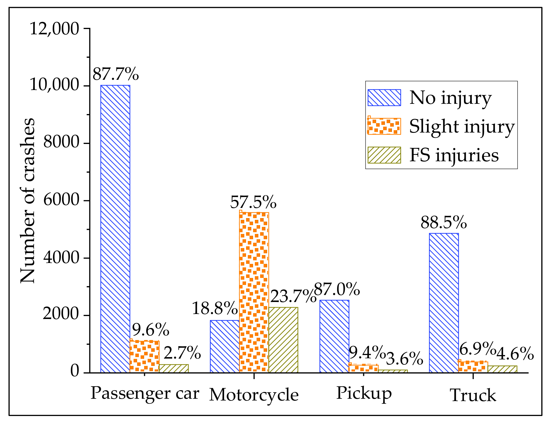
Figure 1. Map of region under study.
Applsci 11 07819 g001
Figure 2. Statistics of crash severity by vehicle types.
Applsci 11 07819 g002
Figure 3. Coefficients of Pearson’s correlation test.
Applsci 11 07819 g003
Figure 4. Average marginal effect of significant risk variables.
Applsci 11 07819 g004
Table 1. Descriptive statistics of model variables across vehicle types.
VariablesCategoriesCount(Ratio/%)
Passenger CarMotorcyclePickupTruck
Number 11,419970329135489
Driver genderMale9858 (86.3)8995 (92.7)2734 (93.8)5478 (99.7)
Female *1561 (13.7)708 (7.2)179 (6.1)11 (0.2)
Driver age<303515 (30.8)2204 (22.7)783 (26.9)687 (12.5)
30–60 *6214 (54.4)4064 (41.8)1722 (59.1)4219 (76.8)
>601690 (14.8)3435 (35.4)408 (14.0)583 (10.6)
Drunk drivingYes1718 (15.0)2512 (25.8)264 (9.1)33 (0.6)
No *9701 (85.0)7191 (74.2)2649 (90.9)5456 (99.4)
WeatherNon-clear1575 (13.7)1219 (12.5)445 (15.3)866 (15.7)
Clear *9844 (86.2)8484 (87.4)2468 (84.7)4623 (84.2)
Road surfaceNon-dry1293 (11.3)984 (10.1)315 (10.8)632 (11.5)
Dry *10,126 (88.7)8719 (89.9)2598 (89.2)4857 (88.5)
Crash typeNon-fixed object *8984 (78.6)7766 (80.0)2252 (77.3)4058 (73.9)
Fixed object838 (7.3)1087 (11.2)188 (6.4)937 (17.0)
Collision with pedestrian1492 (13.0)766 (7.8)434 (14.8)445 (8.1)
Others105 (0.9)84 (0.8)39 (1.3)49 (0.8)
WeekMonday–Tuesday3314 (29.0)2780 (28.7)844 (29.0)1525 (27.8)
Wednesday *1591 (13.9)1419 (14.6)419 (14.3)767 (13.9)
Thursday–Friday3330 (29.2)2810 (29.0)841 (28.9)1653 (30.1)
Weekend3184 (27.9)2694 (27.7)809 (27.8)1544 (28.2)
MonthEarly in month3788 (33.1)3145 (32.4)933 (32.0)1783 (32.4)
Middle in month *3730 (32.7)3249 (33.5)965 (33.2)1809 (33.0)
Late in month3901 (34.2)3309 (34.1)1015 (34.8)1897 (34.6)
SeasonSpring *2872 (25.2)2632 (27.1)762 (26.1)1532 (27.9)
Summer2805 (24.6)2539 (26.1)676 (23.2)1415 (25.7)
Fall3094 (27.0)2614 (26.9)782 (26.8)1573 (28.6)
Winter2648 (23.1)1918 (19.8)693 (23.8)969 (17.7)
LightDaylight *7314 (64.0)6011 (61.9)1966 (67.5)2946 (53.6)
Dark (with street lighting)2485 (21.7)1661 (17.1)465 (15.9)798 (14.5)
Dark (without street lighting)1620 (14.2)2031 (20.9)482 (16.5)1745 (31.7)
Crash timeDay *6561 (57.5)5345 (55.1)1780 (61.1)2550 (46.5)
Night4858 (42.5)4358 (44.9)1133 (38.9)2939 (53.5)
TrafficControlled7603 (66.5)6376 (65.7)1874 (64.3)3668 (66.8)
controlUncontrolled *3816 (33.4)3327 (34.2)1039 (35.6)1821 (33.1)
Note: * indicates that variable was reference variable in model.
Table 2. Characteristics statistics of crash severity model proposed in this research.
ModelsTypesCharacteristics
MN-logit modelFixed effects modelCannot capture unobserved heterogeneity and spatial correlation.
RP-logit modelRandom effects
model
Captures unobserved heterogeneity by allowing parameters of risk factors to vary randomly and cannot capture spatial correlation.
RI-logit modelCaptures unobserved heterogeneity by only allowing the intercept to vary randomly and cannot capture spatial correlation.
SRP-logit modelCaptures unobserved heterogeneity by allowing parameters of risk factors to vary randomly and captures spatial correlation by structured spatial error term.
Table 3. Comparison results of model diagnosis.
IndexMN-Logit ModelRP-Logit ModelRI-Logit ModelSRP-Logit Model
PAMOPITRPAMOPITRPAMOPITRPAMOPITR
D ¯ 8797859921044176871284962037411287568553206841588683847920144067
pD62585154115119919383786973138131112117
DIC8859865721554230882786152128420588398631213742178821861021264184
CA1/%79.522.068.175.282.530.273.679.181.229.469.574.184.636.479.181.3
CA2/%28.164.917.429.126.373.020.830.127.362.015.432.932.280.527.630.7
CA3/%6.428.19.211.610.433.98.918.79.529.110.716.516.038.215.222.6
CAwhole/%72.647.961.568.375.255.766.372.174.148.562.368.279.162.175.874.5
Note: PA = Passenger car; MO = Motorcycle; PI = Pickup; TR = Truck.
Table 4. Estimation of the parameters of the MN-logit model and the RI-logit model.
VariablesMN-Logit ModelRI-Logit Model
PAMOPITRPAMOPITR
Male0.320 **–0.150 ***0.160 **0.311 **–0.139 ***0.142 *
No-–clear−0.435 *0.305 **−0.284 *−0.250 **−0.442 *0.317 **−0.253 *−0.241 *
Controlled0.174 *0.177 *
Age > 600.334 **0.376 ***0.488 **0.342 **0.351 ***0.504 **
Drunk driving0.345 ***0.161 ***1.349 **0.339 ***0.159 ***1.296 ***
Weekend0.087 *0.154 *0.710 *0.235 **0.101 *0.147 *0.716 *
Early in month0.161 *−0.172 **0.157*−0.178 **
Late in month0.157 *0.161 *
Fall−0.071 *−0.246 *−0.083 *−0.239 *
Winter0.376 *0.144 *0.198 *0.395 *0.160 **0.202 *
Dark (with street lighting)0.327 **0.355 *
Dark (without street lighting)0.831 *0.349 *0.708 *0.718 **0.836 *0.352 **0.764 *0.737 *
Collision with fixed object1.231 **1.105 ***1.315 *0.498 *1.248 **1.124 ***1.307 **0.510 *
Collision with pedestrian−2.126 **−2.401 *−1.125 *−1.105 **−2.092 **−2.437 *−1.164 *−1.094 ***
Intercept−2.441 **0.698 *−2.273 *−1.386 ***−2.608 **0.762 **−2.494 *−1.327 ***
s.d. intercept0.6320.4550.3180.269
Note: * indicates 90% credit interval; ** indicates 95% credit interval; *** indicates a credit interval above 95%; “–” indicates that the risk factor is insignificant or is not included in the model.
Table 5. Estimation of the parameters of the RP-logit model and the SRP-logit model.
VariablesRP-Logit ModelSRP-Logit Model
PAMOPITRPAMOPITR
Male0.317 **−0.144 ***0.157 *0.315 **−0.147 ***0.152 *
s.d. male1.2180.4970.9371.1970.5031.043
Non–clear−0.447 *0.312 **−0.255*−0.236 *−0.439*0.342 ***−0.261 *−0.239 *
s.d. non–clear0.1340.1070.5130.1400.2100.522
Controlled0.181 *
Age > 600.340 **0.349 ***0.494 **0.357 **0.346 ***0.473 **
Drunk driving0.340 ***0.166 ***1.251 ***0.343 **0.163 ***1.248 ***
s.d. drunk driving1.5521.408
Weekend0.237 **0.105 *0.165 *0.712 *0.232 **0.092 *0.151 *0.707 **
s.d. weekend0.3711.0300.4011.206
Early in month0.167*−0.169 **0.165 *−0.167 **
Late in month0.168 *0.165 *
Fall−0.066 *−0.232 *−0.057 *−0.238 *
Winter0.393 **0.168 **0.227 *0.358**0.157 **0.219*
Dark(with street lighting)0.324 *
Dark(without street lighting)0.847 *0.341 **0.693 *0.769 *0.845 *0.347 **0.725 *0.771 *
Collision with fixed object1.257 **1.151 ***1.240 *0.509 *1.268 **1.147 ***1.251 *0.512 *
Collision with pedestrian−2.125 **−2.409 *−1.094 **−1.065 ***−2.157 **−2.416 *−1.119 **−1.061 ***
Intercept−2.637 **0.519 *−2.179 *−1.270 ***−2.590 ***0.507 *−2.165 **−1.238 ***
τ s 1 0.7120.7230.595
τ s 2 0.5430.6910.749
τ s 3 0.850
Note: * indicates 90% credit interval; ** indicates 95% credit interval; *** indicates a credit interval above 95%; “–” indicates that the risk factor is insignificant or is not included in the model.
Table 6. The calculation results of model transferability.
Application DataEstablished Model
Passenger CarMotorcyclePickupTruck
Passenger car1−1.2600.329−0.895
Motorcycle−0.3781−0.437−1.139
Pickup0.417−0.9171−0.743
Truck−0.129−2.031−0.1541
Publisher’s Note: MDPI stays neutral with regard to jurisdictional claims in published maps and institutional affiliations.

