
Augmented Data and XGBoost Improvement for Sales Forecasting in the Large-Scale Retail Sector


Abstract
:1. Introduction
- -
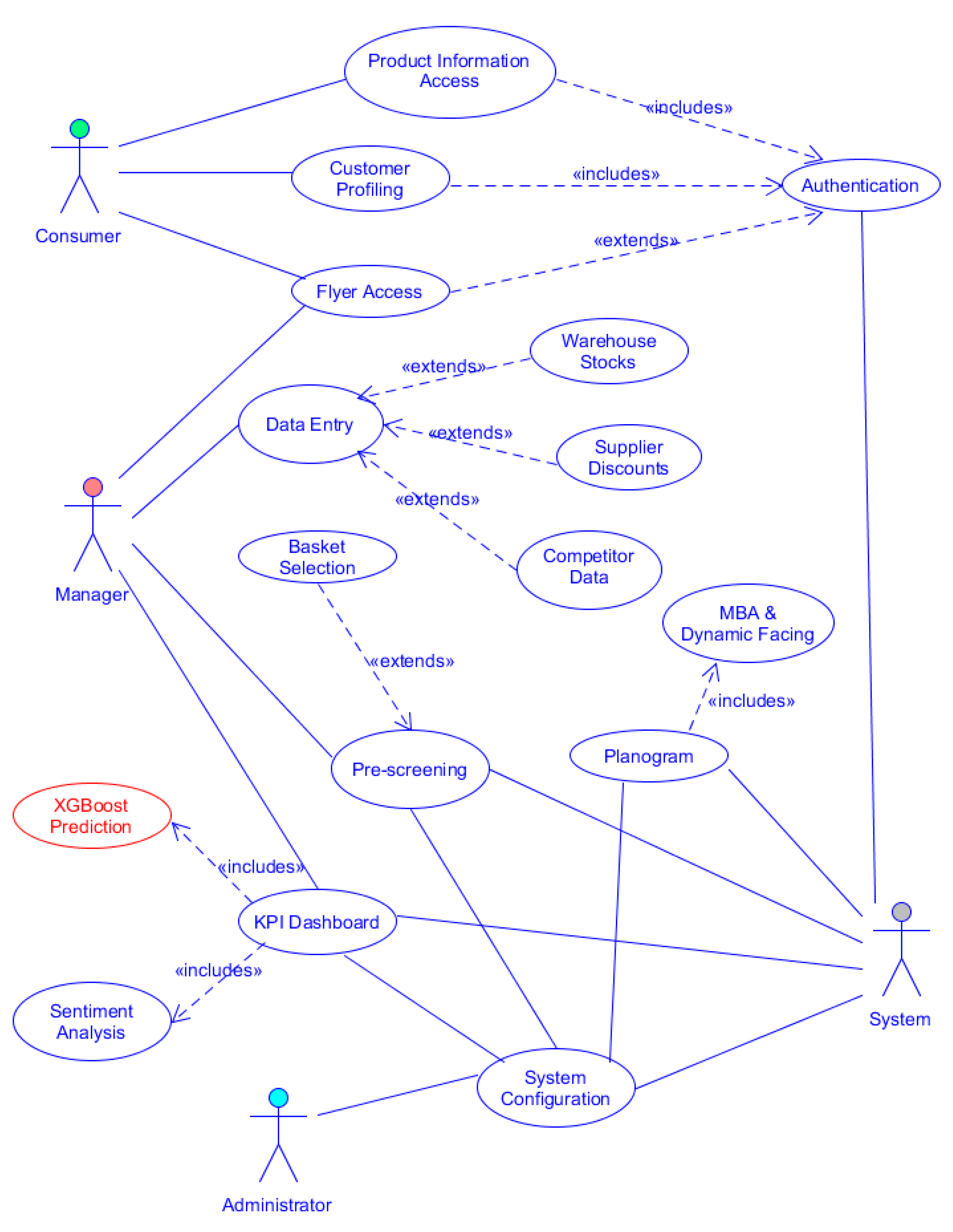
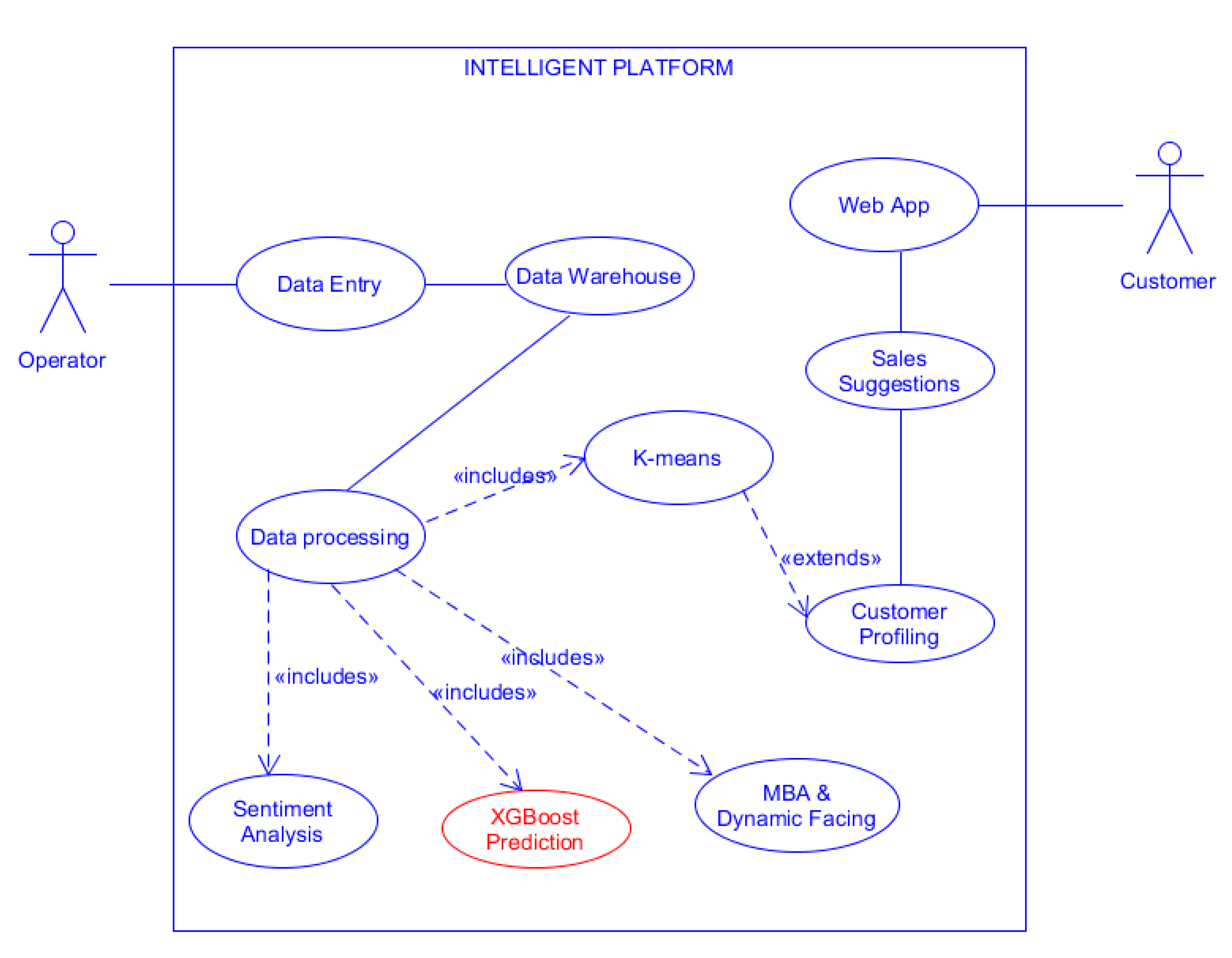
- the DSS platform main functions are defined;
- -
- the multiple attributes influencing the supermarket sales predictions are defined;
- -
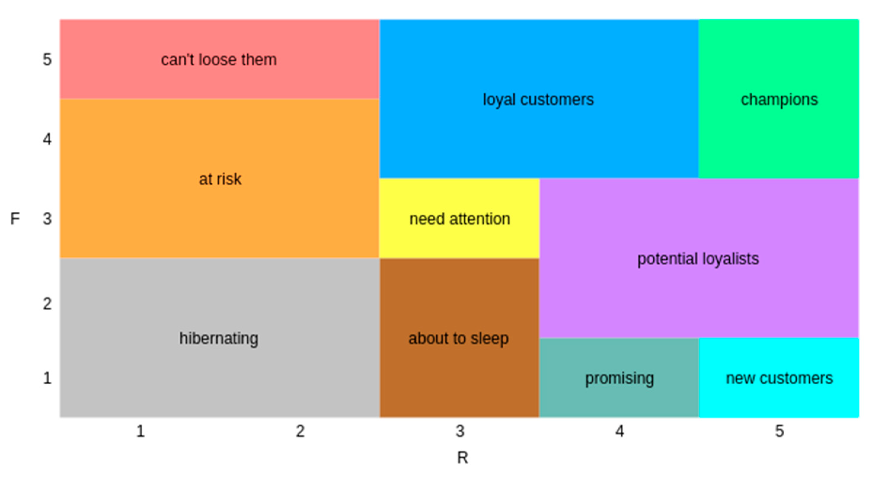
- the customer grid (customer segmentation) is structured;
- -
- the AD approach able to increase the DSS performance is defined;
- -
- the platform is implemented;
- -
- the XGBoost algorithm is tested by proving the correct choice of the AD approach for the DSS.
2. Methodology: Platform Design and Implementation and AD Approach
2.1. Platform Design and Implementation
- -
- day of purchase of the product;
- -
- week number;
- -
- promotion status;
- -
- weather conditions;
- -
- perceived temperature;
- -
- ratio between the number of receipts containing the specific product code and the number of receipts sold in total during the day;
- -
- ratio between the number of customer receipts with the cluster identified and the total number of receipts for the day;
- -
- ratio between the total receipts issued by the department of the specific product code and the number of total receipts issued during the day;
- -
- unit price;
- -
- ratio between the number of customers who bought that product and the total number of customers of the day;
- -
- total number of customers of the day;
- -
- product in promotion at the competitor;
- -
- holiday week;
- -
- week before a holiday week;
- -
- holiday;
- -
- day after a holiday;
- -
- pre-holiday;
- -
- closing day of the financial year.
- one hot encoding, which is a mechanism that consists of transforming the input data into binary code;
- clustering, in order to obtain a relevant statistic, the clientele was divided into groups of customers with similar habits.
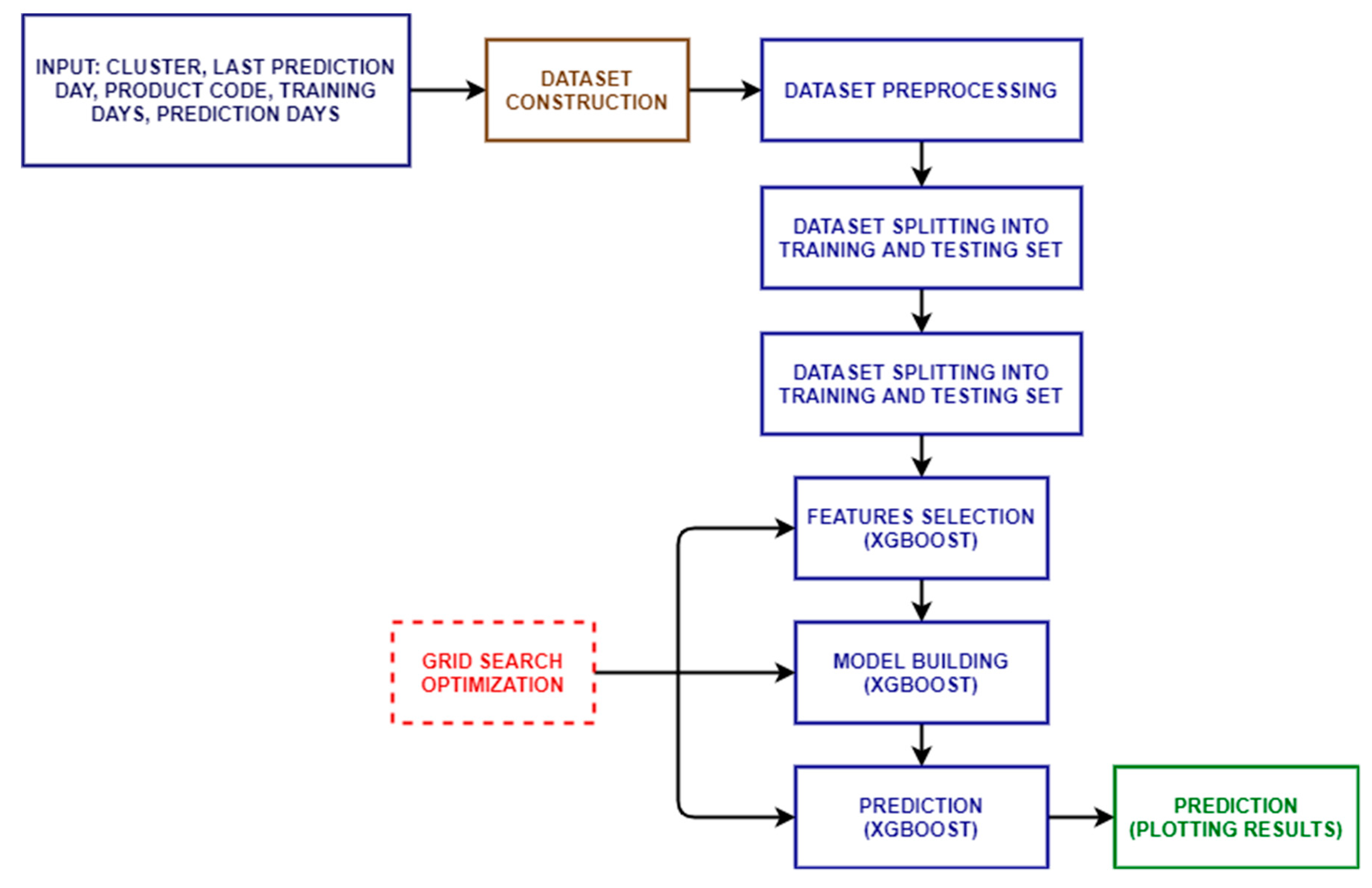
2.2. XGBoost Algorithm
- -
- Numpy, which facilitates the use of large matrices and multidimensional arrays to operate effectively on data structures by means of high-level mathematical functions;
- -
- Pandas, which allows the manipulation and analysis of data;
- -
- XGBoost, which provides a gradient boosting framework;
- -
- Sklearn, which provides various supervised and unsupervised learning algorithms.
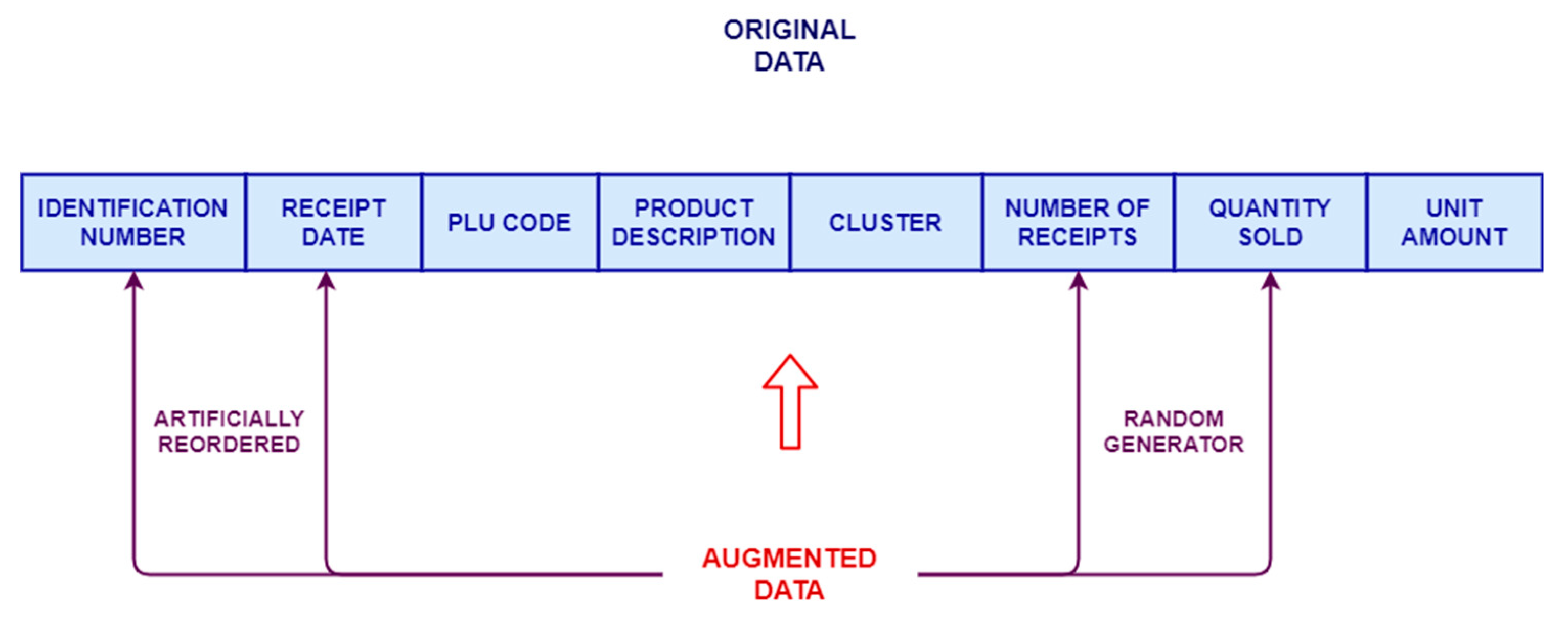
2.3. AD Approach Applied for Large-Scale Retail Sector
- receipt identification code
- receipt date
- customer cluster
- plu code
- day of the week
- week
- quantity sold (number of items)
- eventual promotion
- store branch identifier
- unit amount
- measured quantity (kg)
- product description
- number of receipts
- shop department identifier
3. Results and Discussion
- various foodstuffs (food and drinks, such as flour, pasta, rice, tomato sauce, biscuits, wine, vinegar, herbal teas, water, etc.);
- delicatessen department (cured meats and dairy products);
- fruit and vegetables (fresh fruit and vegetables, packaged vegetables);
- bakery (bread, taralli, grated bread, bread sticks, etc.);
- household products (napkins, handkerchiefs, toothpicks, shower gels, toothpaste, pet food, etc.);
- frozen products (peas, minestrone, ice cream, etc.);
- refrigerator packaged products (fresh milk, butter, dairy products, cheeses, packaged meats, etc.).
- cream pack, flour pack, still water bottle, iodized sea salt pack;
- mozzarella;
- loose tomatoes;
- bread;
- paper towel;
- frozen soup;
- bottle of fresh milk, smoked scarmorze.
4. Conclusions
Author Contributions
Funding
Institutional Review Board Statement
Informed Consent Statement
Data Availability Statement
Acknowledgments
Conflicts of Interest
Appendix A

| model = XGBRegressor(booster = ‘gbtree’, n_jobs = −1, |
| learning_rate = gsearch234fin.best_params_[‘learning_rate’], |
| objective = ‘reg:squarederror’, |
| n_estimators = n_estimators_fit, max_depth = max_depth_fit, |
| min_child_weight = min_child_weight_fit, gamma = gamma_fit, |
| alpha = alpha_fit, |
| reg_lambda = reg_lambda_fit, subsample = subsample_fit, |
| colsample_bytree = colsample_bytree_fit, |
| seed = 26) |
| gsearch234 = GridSearchCV( |
| estimator = XGBRegressor(booster = ‘gbtree’, n_jobs = −1, objective = ‘reg:squarederror’, |
| learning_rate = learning_rate_fit, |
| n_estimators = n_estimators_fit, |
| max_depth = max_depth_fit, subsample = subsample_fit, |
| colsample_bytree = colsample_bytree_fit, |
| min_child_weight = min_child_weight_fit, |
| gamma = gamma_fit, alpha = 0, reg_lambda = 1, |
| seed = 27), |
| param_grid = param_test234, iid = False, cv = 3, scoring = ‘neg_mean_squared_error’) |
| gsearch234.fit(selected_xtraintesttrain, selected_ytraintesttrain) |
References
- Raschka, S.; Mirjalili, V. Python Machine Learning, 3rd ed.; Packt: Birmingham, UK, 2019; p. 725. ISBN 978-1-78995-575-0. [Google Scholar]
- Zinoviev, D. Data Science Essentials in Python Collect → Organize → Explore → Predict → Value. The Pragmatic Bookshelf, 2016. Available online: https://pragprog.com/titles/dzpyds/data-science-essentials-in-python/ (accessed on 22 July 2021).
- Massaro, A.; Panarese, A.; Dipierro, G.; Cannella, E.; Galiano, A. Infrared Thermography and Image Processing applied on Weldings Quality Monitoring. In Proceedings of the IEEE International Workshop on Metrology for Industry 4.0 & IoT, Roma, Italy, 3–5 June 2020; pp. 559–564. [Google Scholar] [CrossRef]
- Palmer, A.; Jiménez, R.; Gervilla, E. Data Mining: Machine Learning and Statistical Techniques. In Knowledge-Oriented Applications in Data Mining; 2011; Available online: https://www.intechopen.com/books/1358 (accessed on 22 July 2021).
- Shmueli, G.; Patel, N.R.; Bruce, P.C. Data Mining for Business Intelligence. Concepts, Techniques, and Applications in Microsoft Office Excel with XLMiner; John Wiley & Sons: New Jersey, NJ, USA, 2007. [Google Scholar]
- Massaro, A.; Panarese, A.; Selicato, S.; Galiano, A. CNN-LSTM Neural Network Applied for Thermal Infrared Underground Water Leakage. In Proceedings of the IEEE International Workshop on Metrology for Industry 4.0 & IoT (MetroInd4.0&IoT), Rome, Italy, 7–9 June 2021; pp. 219–224. [Google Scholar] [CrossRef]
- Massaro, A.; Panarese, A.; Galiano, A. Technological Platform for Hydrogeological Risk Computation and Water Leakage Detection based on a Convolutional Neural Network. In Proceedings of the IEEE International Workshop on Metrology for Industry 4.0 & IoT (MetroInd4.0&IoT), Rome, Italy, 7–9 June 2021; pp. 225–230. [Google Scholar] [CrossRef]
- Davenport, T.H. Competing on Analytics. Harvard Business Review. Harv. Bus. Rev. 2006, 84, 98–107. [Google Scholar] [PubMed]
- Massaro, A.; Galiano, A.; Barbuzzi, D.; Pellicani, L.; Birardi, G.; Romagno, D.D.; Frulli, L. Joint Activities of Market Basket Analysis and Product Facing for Business Intelligence oriented on Global Distribution Market: Examples of Data Mining Applications. Int. J. Comput. Sci. Inform. Technol. 2017, 8, 178–183. [Google Scholar]
- Salonen, J.; Pirttimaki, V. Outsourcing a Business Intelligence Function. FeBR 2005, Frontiers of e-Business Research, 2005. Available online: https://researchportal.tuni.fi/en/publications/outsourcing-a-business-intelligence-function (accessed on 3 August 2021).
- Turban, E.; Aronson, J.E. Decision Support Systems and Intelligent Systems, 6th ed.; Prentice-Hall: Hoboken, NJ, USA, 2001. [Google Scholar]
- Aguasca-Colomo, R.; Castellanos-Nieves, D.; Méndez, M. Comparative Analysis of Rainfall Prediction Models Using Machine Learning in Islands with Complex Orography: Tenerife Island. Appl. Sci. 2019, 9, 4931. [Google Scholar] [CrossRef] [Green Version]
- Liu, Z.; Yang, J.; Jiang, W.; Wei, C.; Zhang, P.; Xu, J. Research on Optimized Energy Scheduling of Rural Microgrid. Appl. Sci. 2019, 9, 4641. [Google Scholar] [CrossRef] [Green Version]
- Phan, Q.; Wu, Y.K.; Phan, Q. A Hybrid Wind Power Forecasting Model with XGBoost, Data Preprocessing Considering Different NWPs. Appl. Sci. 2021, 11, 1100. [Google Scholar] [CrossRef]
- Zheng, H.; Wu, Y. A XGBoost Model with Weather Similarity Analysis and Feature Engineering for Short-Term Wind Power Forecasting. Appl. Sci. 2019, 9, 3019. [Google Scholar] [CrossRef] [Green Version]
- Wei, H.; Zeng, Q. Research on sales Forecast based on XGBoost-LSTM algorithm Model. J. Phys. Conf. Ser. 2021, 1754, 012191. [Google Scholar] [CrossRef]
- Pavlyshenko, B.M. Machine-Learning Models for Sales Time Series Forecasting. Data 2019, 4, 15. [Google Scholar] [CrossRef] [Green Version]
- Chang, W.; Liu, Y.; Xiao, Y.; Xu, X.; Zhou, S.; Lu, X.; Cheng, Y. Probability Analysis of Hypertension-Related Symptoms Based on XGBoost and Clustering Algorithm. Appl. Sci. 2019, 9, 1215. [Google Scholar] [CrossRef] [Green Version]
- Yu, L.; Mu, Q. Heart Disease Prediction Based on Clustering and XGboost Algorithm. Comput. Syst. Appl. 2019, 28, 228–232. [Google Scholar]
- Li, M.; Fu, X.; Li, D. Diabetes Prediction Based on XGBoost Algorithm. IOP Conf. Ser. Mater. Sci. Eng. 2020, 768. [Google Scholar] [CrossRef]
- Gumus, M.; Kıran, M.S. Crude Oil Price Forecasting Using XGBoost. In Proceedings of the International Conference on Computer Science and Engineering (UBMK), Antalya, Turkey, 5–8 October 2017; pp. 1100–1103. [Google Scholar] [CrossRef]
- Shi, X.; Li, Q.; Qi, Y.; Huang, T.; Li, J. An accident prediction approach based on XGBoost. In Proceedings of the 12th International Conference on Intelligent Systems and Knowledge Engineering (ISKE), Nanjing, China, 24–26 November 2017; pp. 1–7. [Google Scholar] [CrossRef]
- Massaro, A.; Dipierro, G.; Saponaro, A.; Galiano, A. Data Mining Applied in Food Trade Network. Int. J. Artif. Intell. Appl. 2020, 11, 15–35. [Google Scholar] [CrossRef]
- Massaro, A.; Galiano, A. Re-Engineering Process in a Food Factory: An Overview of Technologies and Approaches for the Design of Pasta Production Processes. Prod. Manuf. Res. 2020, 8, 80–100. [Google Scholar] [CrossRef] [Green Version]
- Massaro, A.; Selicato, S.; Miraglia, R.; Panarese, A.; Calicchio, A.; Galiano, A. Production Optimization Monitoring System Implementing Artificial Intelligence and Big Data. In Proceedings of the IEEE International Workshop on Metrology for Industry 4.0 & IoT, Roma, Italy, 3–5 June 2020; pp. 570–575. [Google Scholar] [CrossRef]
- Galiano, A.; Massaro, A.; Barbuzzi, D.; Pellicani, L.; Birardi, G.; Boussahel, B.; De Carlo, F.; Calati, V.; Lofano, G.; Maffei, L.; et al. Machine to Machine (M2M) Open Data System for Business Intelligence in Products Massive Distribution oriented on Big Data. Int. J. Comput. Sci. Inform. Technol. 2016, 7, 1332–1336. [Google Scholar]
- Massaro, A.; Maritati, V.; Galiano, A. Data Mining Model Performance of Sales Predictive Algorithms Based on Rapidminer Workflows. Int. J. Comput. Sci. Inf. Technol. 2018, 10, 39–56. [Google Scholar] [CrossRef]
- Massaro, A.; Barbuzzi, D.; Vitti, V.; Galiano, A.; Aruci, M.; Pirlo, G. Predictive Sales Analysis According to the Effect of Weather. In Proceedings of the 2nd International Conference on Recent Trends and Applications in Computer Science and Information Technology, Tirana, Albania, 18–19 November 2016; pp. 53–55. [Google Scholar]
- Massaro, A.; Vitti, V.; Galiano, A.; Morelli, A. Business Intelligence Improved by Data Mining Algorithms and Big Data Systems: An Overview of Different Tools Applied in Industrial Research. Comput. Sci. Inf. Technol. 2019, 7, 1–21. [Google Scholar] [CrossRef]
- Massaro, A.; Vitti, V.; Mustich, A.; Galiano, A. Intelligent Real-time 3D Configuration Platform for Customizing E-commerce Products. Int. J. Comput. Graph. Animat. 2019, 9, 13–28. [Google Scholar] [CrossRef]
- Masaro, A.; Mustich, A.; Galiano, A. Decision Support System for Multistore Online Sales Based on Priority Rules and Data Mining. Comput. Sci. Inf. Technol. 2020, 8, 1–12. [Google Scholar] [CrossRef]
- El-Bialy, R.; Salamay, M.A.; Karam, O.H.; Khalifa, M.E. Feature Analysis of Coronary Artery Heart Disease Data Sets. Procedia Comput. Sci. 2015, 65, 459–468. [Google Scholar] [CrossRef] [Green Version]
- Sabay, A.; Harris, L.; Bejugama, V.; Jaceldo-Siegl, K. Overcoming Small Data Limitations in Heart Disease Prediction by Using Surrogate Data. SMU Data Sci. Rev. 2018, 1. Available online: https://scholar.smu.edu/datasciencereview/vol1/iss3/12 (accessed on 22 July 2021).
- Li, H.; Xiong, L.; Jiang, X. Differentially Private Synthesization of Multi-Dimensional Data using Copula Functions. Adv Database Technol. 2014, 475–486. [Google Scholar] [CrossRef]
- Akshay, K.; Akhilesh, V.; Animikh, A.; Chetana, H. Sales-Forecasting of Retail Stores using Machine Learning Techniques. In Proceedings of the 3rd IEEE International Conference on Computational Systems and Information Technology for Sustainable Solutions, Bengaluru, India, 20–22 December 2018; pp. 160–166. [Google Scholar] [CrossRef]
- Huang, W.; Zhang, Q.; Xu, W.; Fu, H.; Wang, M.; Liang, X. A Novel Trigger Model for Sales Prediction with Data Mining Techniques. Data Sci. J. 2015, 14. [Google Scholar] [CrossRef]
- Gao, M.; Xu, W.; Fu, H.; Wang, M.; Liang, X. A Novel Forecasting Method for Large-Scale Sales Prediction Using Extreme Learning Machine. In Proceedings of the Seventh International Joint Conference on Computational Sciences and Optimization, Beijing, China, 4–6 July 2014; pp. 602–606. [Google Scholar] [CrossRef]
- Kuo, R.; Xue, K. A Decision Support System for Sales Forecasting through Fuzzy Neural Networks with Asymmetric Fuzzy Weights. Decis. Support Syst. 1998, 24, 105–126. [Google Scholar] [CrossRef]
- Hill, T.; Marquez, L.; O’Connor, M.; Remus, W. Artificial Neural Network Models for Forecasting and Decision Making. Int. J. Forecast. 1994, 10, 5–15. [Google Scholar] [CrossRef] [Green Version]
- Liu, C.-J.; Huang, T.-S.; Ho, P.-T.; Huang, J.-C.; Hsieh, C.-T. Machine Learning-Based E-Commerce Platform Repurchase Customer Prediction Model. PLoS ONE 2020, 15, e0243105. [Google Scholar] [CrossRef]
- Ji, S.; Wang, X.; Zhao, W.; Guo, D. An Application of a Three-Stage XGBoost-Based Model to Sales Forecasting of a Cross-Border E-Commerce Enterprise. Math. Probl. Eng. 2019, 2019, 1–15. [Google Scholar] [CrossRef] [Green Version]
- Song, P.; Liu, Y. An XGBoost Algorithm for Predicting Purchasing Behaviour on E-Commerce Platforms. Teh. Vjesn. Tech. Gaz. 2020, 27, 1467–1471. [Google Scholar] [CrossRef]
- Massaro, A.; Panarese, A.; Gargaro, M.; Vitale, C.; Galiano, A.M. Implementation of a Decision Support System and Business Intelligence Algorithms for the Automated Management of Insurance Agents Activities. Int. J. Artif. Intell. Appl. 2021, 12, 1–13. [Google Scholar] [CrossRef]
- Massaro, A.; Maritati, V.; Giannone, D.; Convertini, D.; Galiano, A. LSTM DSS Automatism and Dataset Optimization for Diabetes Prediction. Appl. Sci. 2019, 9, 3532. [Google Scholar] [CrossRef] [Green Version]
- Massaro, A.; Panarese, A.; Gargaro, M.; Colonna, A.; Galiano, A. A Case Study of Innovation in the Implementation of a DSS System for Intelligent Insurance Hub Services. Comput. Sci. Inform. Technol. 2021, 9, 14–23. [Google Scholar] [CrossRef]
- Shcherbakov, M.V.; Brebels, A.; Shcherbakova, N.L.; Tyukov, A.P.; Janovsky, T.A.; Kamaev, V.A. A Survey of Forecast Error Measures. World Appl. Sci. J. 2013, 24, 171–176. [Google Scholar] [CrossRef]
- Syntetos, A.A.; Boylan, J.E. The Accuracy of Intermittent Demand Estimates. Int. J. Forecast. 2004, 21, 303–314. [Google Scholar] [CrossRef]
- Mishra, P.; Passos, D. A Synergistic Use of Chemometrics and Deep Learning Improved the Predictive Performance of near-Infrared Spectroscopy Models for Dry Matter Prediction in Mango Fruit. Chemom. Intell. Lab. Syst. 2021, 212, 104287. [Google Scholar] [CrossRef]
- Panarese, A.; Bruno, D.; Colonna, G.; Diomede, P.; Laricchiuta, A.; Longo, S.; Capitelli, M. A Monte Carlo Model for determination of binary diffusion coefficients in gases. J. Comput. Phys. 2011, 230, 5716–5721. [Google Scholar] [CrossRef]
- Upadhyay, D.; Manero, J.; Zaman, M.; Sampalli, S. Gradient Boosting Feature Selection with Machine Learning Classifiers for Intrusion Detection on Power Grids. IEEE Trans. Netw. Serv. Manag. 2020, 18, 1104–1116. [Google Scholar] [CrossRef]
- Pedregosa, F.; Varoquaux, G.; Gramfort, A.; Michel, V.; Thirion, B.; Grisel, O.; Blondel, M.; Prettenhofer, P.; Weiss, R.; Du-bourg, V.; et al. Scikit-Learn: Machine Learning in Python. J. Mach. Learn. Res. 2015, 12, 2825–2830. [Google Scholar]
- Charoen-Ung, P.; Mittrapiyanuruk, P. Sugarcane Yield Grade Prediction using Random Forest and Gradient Boosting Tree Techniques. In Proceedings of the 15th International Joint Conference on Computer Science and Software Engineering (JCSSE), Nakhon Pathom, Thailand, 11–13 July 2018; pp. 1–6. [Google Scholar] [CrossRef]
- Panarese, A.; Bruno, D.; Tolias, P.; Ratynskaia, S.; Longo, S.; De Angelis, U. Molecular Dynamics Calculation of the Spectral Densities of Plasma Fluctuations. J. Plasma Phys. 2018, 84, 905840308. [Google Scholar] [CrossRef]
- Tolias, P.; Ratynskaia, S.; Panarese, A.; Longo, S.; De Angelis, U. Natural fluctuations in un-magnetized and magnetized plasmas. J. Plasma Phys. 2015, 81, 905810314. [Google Scholar] [CrossRef]
- Twomey, J.; Smith, A. Performance Measures, Consistency, and Power for Artificial Neural Network Models. Math. Comput. Model. 1995, 21, 243–258. [Google Scholar] [CrossRef]
- Phan, Q.-T.; Wu, Y.-K. A Comparative Analysis of XGBoost and Temporal Convolutional Network Models for Wind Power Forecasting. In Proceedings of the International Symposium on Computer, Consumer and Control (IS3C), Taichung City, Taiwan, 13–16 November 2020; pp. 416–419. [Google Scholar] [CrossRef]
- Memon, N.; Patel, S.B.; Patel, D.P. Comparative Analysis of Artificial Neural Network and XGBoost Algorithm for PolSAR Image Classification. In Pattern Recognition and Machine Intelligence; PReMI 2019. Lecture Notes in Computer Science; Deka, B., Maji, P., Mitra, S., Bhattacharyya, D., Bora, P., Pal, S., Eds.; Springer: Basel, Switzerland, 2019; Volume 11941. [Google Scholar] [CrossRef]
- Nelli, F. Machine Learning with Scikit-Learn. Python Data Anal. 2015, 237–264. [Google Scholar] [CrossRef]
- Chen, T.; Guestrin, C. XGBoost: A Scalable Tree Boosting System. In Proceedings of the 22nd ACM SIGKDD International Conference on Knowledge Discovery and Data Mining, San Francisco, CA, USA, 13–17 August 2016; pp. 785–794. [Google Scholar] [CrossRef] [Green Version]
- Massaro, A.; Maritati, V.; Savino, N.; Galiano, A.; Convertini, D.; De Fonte, E.; Di Muro, M. A Study of a Health Resources Management Platform Integrating Neural Networks and DSS Telemedicine for Homecare Assistance. Information 2018, 9, 176. [Google Scholar] [CrossRef] [Green Version]
- Massaro, A.; Vitti, V.; Galiano, A. Model of Multiple Artificial Neural Networks Oriented on Sales Prediction and Product Shelf Design. Int. J. Soft Comput. Artif. Intell. Appl. 2018, 7, 1–19. [Google Scholar] [CrossRef]
| Datum | Number |
|---|---|
| Number of records | 7,212,348 |
| number of daily customers | ~1000 |
| Sampling days | 897 |
| Number of products | 30,159 |
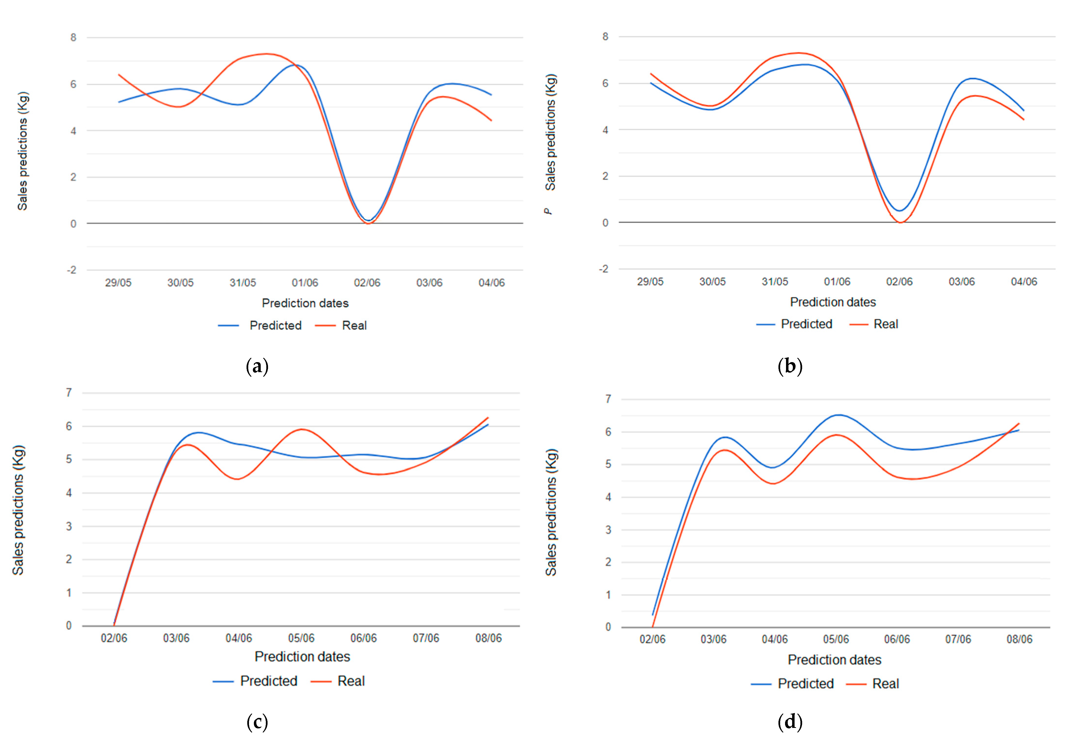
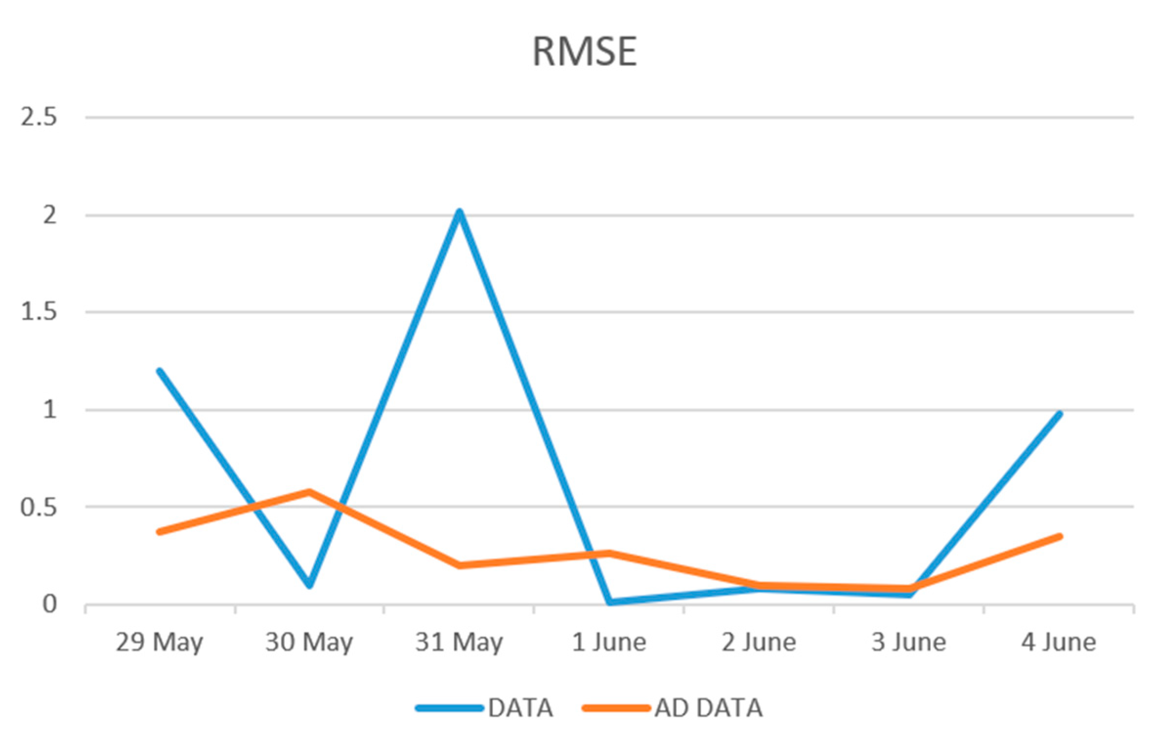
| Accuracy | Original Data | Augmented Data |
|---|---|---|
| RMSE | 0.63 | 0.28 |
| MSE | 0.93 | 0.092 |
| Hyperparameter | Value | Description ([41]) |
|---|---|---|
| Eta (learning_rate) | 0.1 | Learning rate |
| n_estimators | 175 | Number of estimators |
| Max_depth | 2 | Maximum depth of the tree |
| Colsample_bytree | 0.8 | Subsample ratio of columns for each tree |
| Min_child_weight | 1 | Minimum sum of weights in a child |
| Alpha | 0 | Regularization term on weights |
| Lambda | 1 | Regularization term on weights |
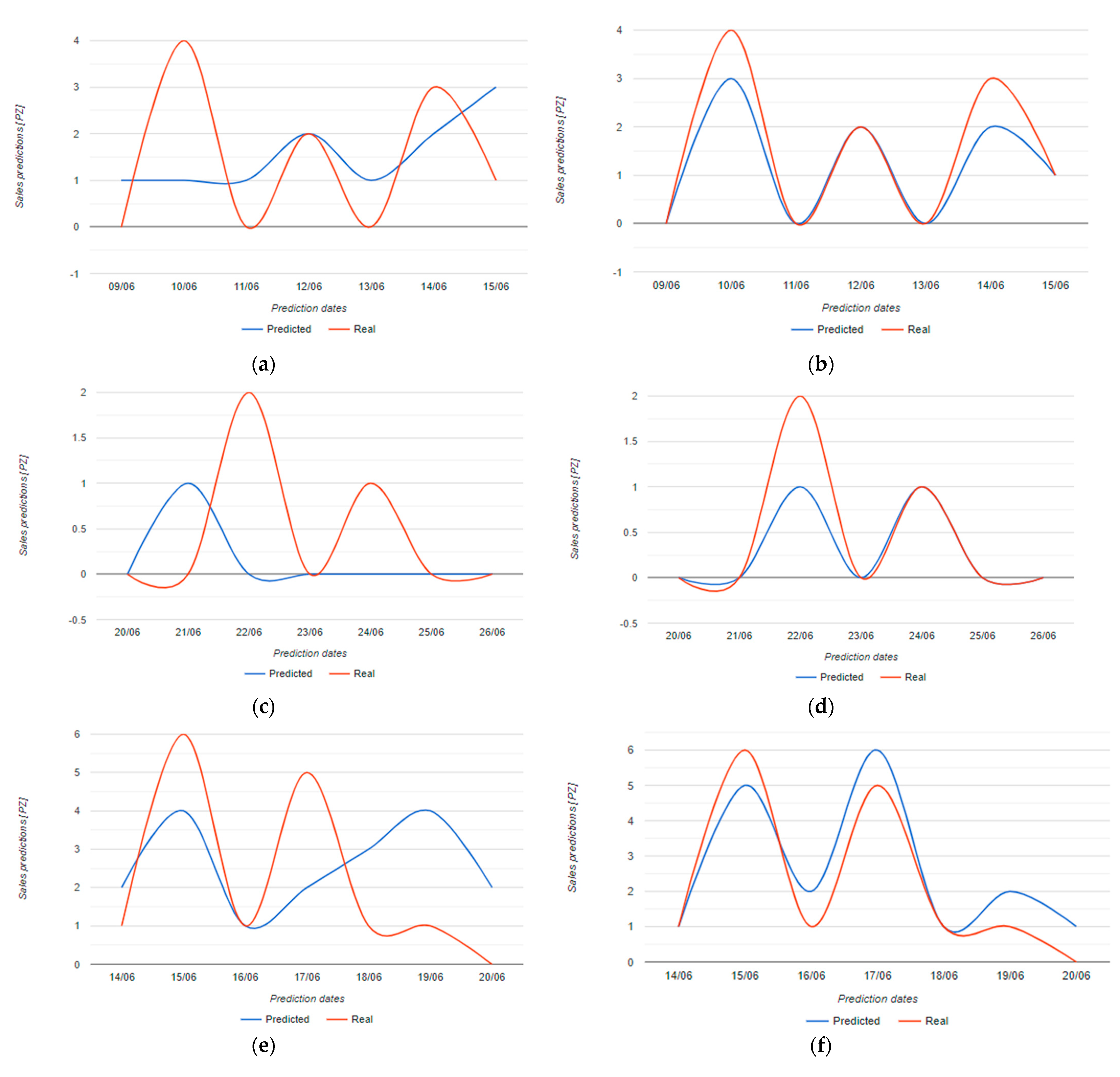
| Item | Original Data RMSE (RMSEP) | Augmented Data RMSE (RMSEP) |
|---|---|---|
| cream (Figure 12a,b) | 1.56 (1.05) | 0.53 (0.16) |
| paper towel (Figure 12c,d) | 0.93 (0.65) | 0.38 (0.19) |
| flour (Figure 12e,f) | 2.10 (1.62) | 0.84 (0.66) |
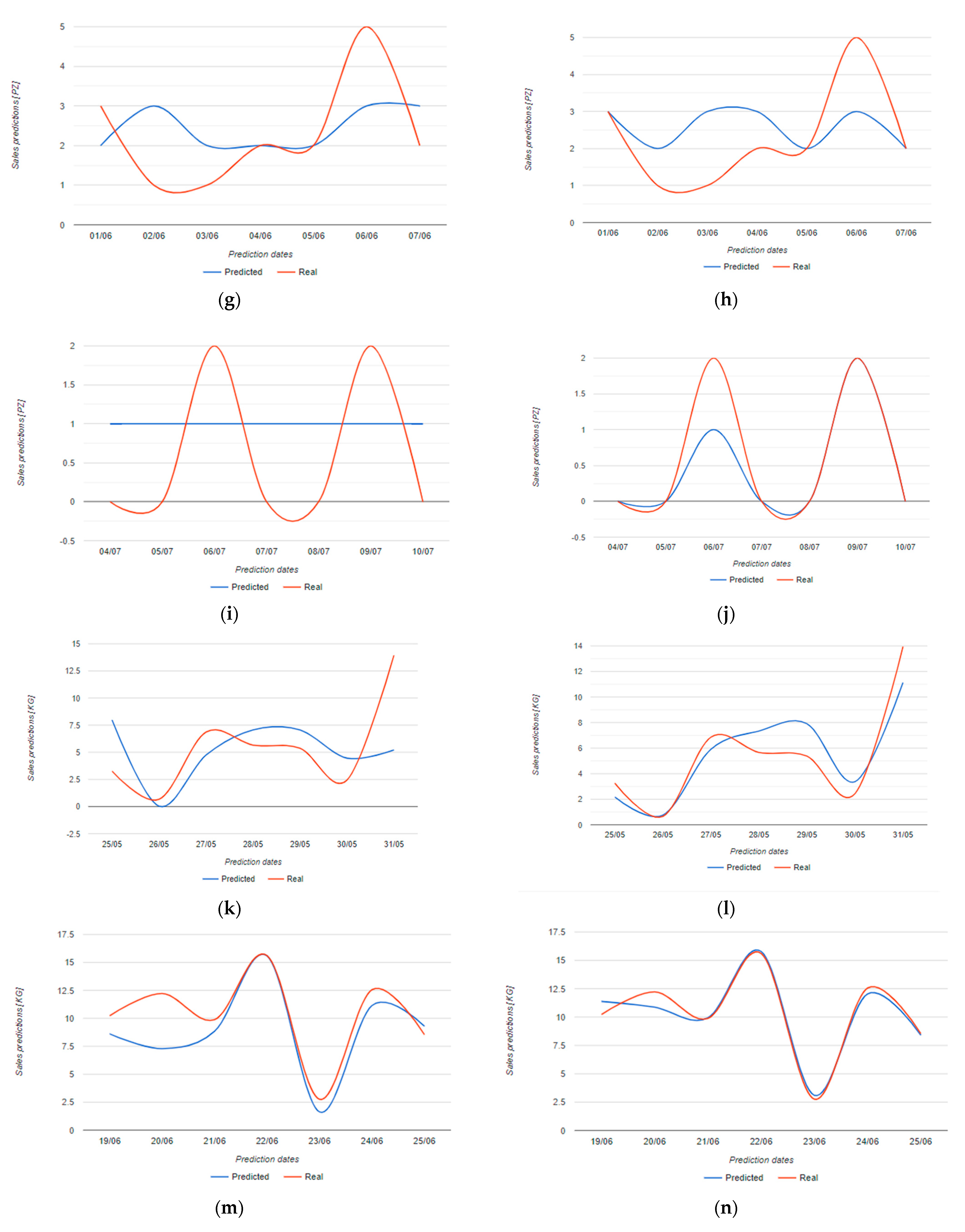
| still water (Figure 12g,h) | 1.25 (0.89) | 1.20 (0.88) |
| sea salt (Figure 12i,j) | 1.00 (0.89) | 0.38 (0.19) |
| tomatoes (Figure 12k,l) | 4.00 (0.79) | 1.70 (0.28) |
| mozzarella (Figure 12m,n) | 2.13 (0.24) | 0.72 (0.072) |
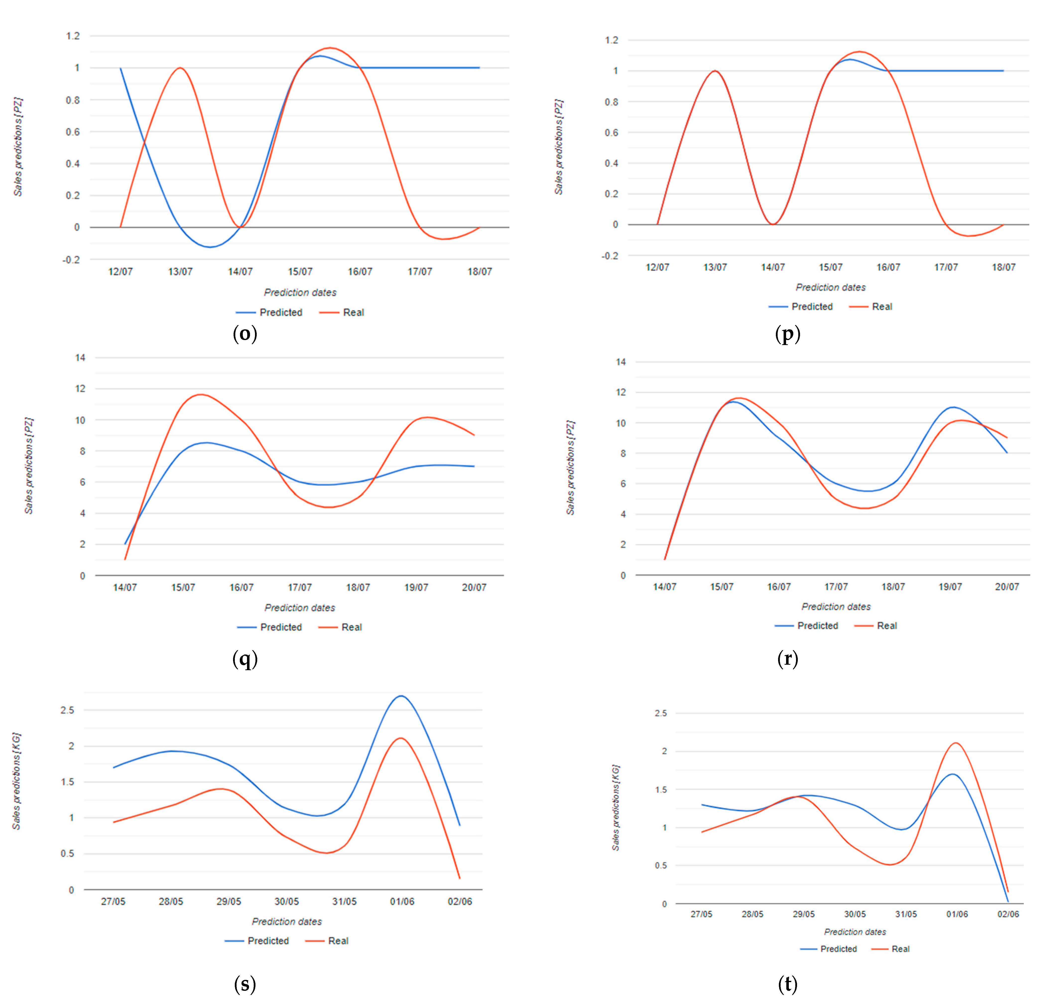
| frozen soup (Figure 12o,p) | 0.76 (0.76) | 0.53 (0.53) |
| fresh milk (Figure 12q,r) | 2.04 (0.44) | 0.85 (0.13) |
| scarmorze (Figure 12s,t) | 0.62 (1.96) | 0.33 (0.40) |
| Item | Original Data Run Time (s) | Augmented Data Run Time (s) |
|---|---|---|
| bread (Figure 9a,b) | 84.54 | 69.77 |
| bread (Figure 9c,d) | 67.61 | 95.28 |
| cream (Figure 12a,b) | 55.69 | 69.65 |
| paper towel (Figure 12c,d) | 70.67 | 68.02 |
| flour (Figure 12e,f) | 79.33 | 62.17 |
| still water (Figure 12g,h) | 57.06 | 61.98 |
| sea salt (Figure 12i,j) | 57.94 | 59.19 |
| tomatoes (Figure 12k,l) | 109.36 | 84.59 |
| mozzarella (Figure 12m,n) | 55.77 | 58.65 |
| frozen soup (Figure 12o,p) | 56.87 | 60.55 |
| fresh milk (Figure 12q,r) | 76.95 | 118.38 |
| scarmorze (Figure 12s,t) | 60.62 | 66.53 |
Publisher’s Note: MDPI stays neutral with regard to jurisdictional claims in published maps and institutional affiliations. |
© 2021 by the authors. Licensee MDPI, Basel, Switzerland. This article is an open access article distributed under the terms and conditions of the Creative Commons Attribution (CC BY) license (https://creativecommons.org/licenses/by/4.0/).
Share and Cite
Massaro, A.; Panarese, A.; Giannone, D.; Galiano, A. Augmented Data and XGBoost Improvement for Sales Forecasting in the Large-Scale Retail Sector. Appl. Sci. 2021, 11, 7793. https://doi.org/10.3390/app11177793
Massaro A, Panarese A, Giannone D, Galiano A. Augmented Data and XGBoost Improvement for Sales Forecasting in the Large-Scale Retail Sector. Applied Sciences. 2021; 11(17):7793. https://doi.org/10.3390/app11177793
Chicago/Turabian StyleMassaro, Alessandro, Antonio Panarese, Daniele Giannone, and Angelo Galiano. 2021. "Augmented Data and XGBoost Improvement for Sales Forecasting in the Large-Scale Retail Sector" Applied Sciences 11, no. 17: 7793. https://doi.org/10.3390/app11177793
APA StyleMassaro, A., Panarese, A., Giannone, D., & Galiano, A. (2021). Augmented Data and XGBoost Improvement for Sales Forecasting in the Large-Scale Retail Sector. Applied Sciences, 11(17), 7793. https://doi.org/10.3390/app11177793