Article

Reinforcement Learning with Self-Attention Networks for Cryptocurrency Trading

Graduate Institute of Automation Technology, National Taipei University of Technology, Taipei 10608, Taiwan
*
Author to whom correspondence should be addressed.
Appl. Sci. 2021, 11(16), 7377; https://doi.org/10.3390/app11167377
Submission received: 10 July 2021 / Revised: 4 August 2021 / Accepted: 10 August 2021 / Published: 11 August 2021
(This article belongs to the Special Issue Machine Learning Techniques for the Study of Complex Systems)

Abstract

:
This work presents an application of self-attention networks for cryptocurrency trading. Cryptocurrencies are extremely volatile and unpredictable. Thus, cryptocurrency trading is challenging and involves higher risks than trading traditional financial assets such as stocks. To overcome the aforementioned problems, we propose a deep reinforcement learning (DRL) approach for cryptocurrency trading. The proposed trading system contains a self-attention network trained using an actor-critic DRL algorithm. Cryptocurrency markets contain hundreds of assets, allowing greater investment diversification, which can be accomplished if all the assets are analyzed against one another. Self-attention networks are suitable for dealing with the problem because the attention mechanism can process long sequences of data and focus on the most relevant parts of the inputs. Transaction fees are also considered in formulating the studied problem. Systems that perform trades in high frequencies cannot overlook this issue, since, after many trades, small fees can add up to significant expenses. To validate the proposed approach, a DRL environment is built using data from an important cryptocurrency market. We test our method against a state-of-the-art baseline in two different experiments. The experimental results show the proposed approach can obtain higher daily profits and has several advantages over existing methods.

1. Introduction

Asset exchange can be very profitable if it is done properly. The values of typically traded assets, such as cryptocurrencies, fluctuate constantly due to the interactions of the participants in markets. Therefore, if it can be predicted which assets have high chances of gaining value, they can be acquired and sold off in the future, generating profits to the investor. Profits can also be generated when the value of assets decreases; short selling and margin trading services work under this premise. Predicting which assets have the potential to increase their value is difficult. This is because trading is linked to human sentiment, which changes rapidly when important global events occur, for instance, political elections, international agreements, or natural disasters, and also it is easily manipulated using branding or marketing campaigns [1]. Nonetheless, asset trading is commonly practiced by both humans and algorithms throughout the world, where the most commonly traded assets are stocks, fiat money, and cryptocurrencies.
In the last decade, cryptocurrencies have gained worldwide relevance despite the initial skepticism of the people towards these assets. More and more countries are allowing the use of cryptocurrencies as a payment method, and in addition, in June of the present year (2021), the republic of El Salvador became the first country to adopt Bitcoin as legal tender. https://www.nytimes.com/2021/06/09/world/americas/salvador-bitcoin.html (accessed on 6 August 2021). However, the price of Bitcoin has been extremely volatile throughout its history, and widely different compared to traditional assets. Therefore, to overcome the shortcomings of this cryptocurrency, hundreds of alternative tokens, known as ‘altcoins’, have sprung up around the world [1], which in turn has made the number of platforms offering cryptocurrency services, such as trading, grow. These platforms have significant advantages against those for other types of assets, with the most important being access to the common public and a minimal amount of cash required to start trading.
We propose a DRL approach for cryptocurrency trading, where a self-attention (SA) network is the backbone of the system. Cryptocurrency markets contain hundreds of assets that can be exchanged. Therefore, being able to process massive amounts of data allows the system to gain a better understanding of the market state and the individual state of the assets, which in turn produces better diversification of investments and reduces risk [2].
This work also explores the problem of inter-asset transactions (IAT). Most markets require a fee for each transaction made on their platforms, and cryptocurrency markets are no exception. Therefore, a tool to compute the transactions that leads to the minimum possible fee expenditure is important. This issue is even more significant if the trading frequency is high, for example, if an investor trades every six hs a cryptocurrency volume worth 10,000 USD with a fixed transaction fee of 0.1%. Then, after only one month the total expenditure would be 1200 USD due to transaction costs, which is a non-trivial amount compared to the traded volume. We study this problem in-depth and propose three algorithms to perform optimal IAT for different applications.
The main contributions of this work are summarized below.
  • A self-attention NN architecture for cryptocurrency trading is proposed. The NN is trained using DRL and is independent of the number of assets in the market.
  • An analysis of the information flow inside the NN is given, explaining how and why the architecture works.
  • The problem of IAT is studied in depth. This includes the description and theoretical justification of three algorithms, and the evaluation of the speed and accuracy of the algorithms.
The rest of the paper is organized as follows. Section 2 discusses the relevant points of related literature. Section 3 presents the mathematical formulation of the problem. Section 4 describes various algorithms that allow the computation of optimal transaction fees. Section 5 describes the deep neural network (NN) architecture used for cryptocurrency trading as well as the training method. Section 6 contains the setup of the experiments implemented to evaluate the performance of our method. Section 7 presents the results of the experiments along with a discussion of the most relevant findings. Finally, conclusions are drawn in Section 8.

2. Literature Review

One of the earliest studies on reinforcement learning applied to asset trading can be found in [3]. In that work, the authors proposed an algorithm named recurrent reinforcement learning (RRL) applied to stock market trading. The authors explored the use of well-known financial measures, such as the Sharpe ratio, as reward functions in the process. Those ideas were expanded in [4], where they compared their approach to other methods. Later on, Gold [5] used a similar approach for currency trading in the foreign exchange (FX) market and focused on comparing different neural networks (NNs) to obtain an optimal architecture for the problem. Dempster and Leemans [6] proposed adaptive reinforcement learning to the FX market. The method is a complex system, in which decisions are based on performance, risk measures, and a dynamic optimization process. Maringer and Ramtohul [7] proposed a threshold RRL method, which uses two networks trained in tandem to deal with two different market states, one for a volatile market and the other for a non-volatile one. They argued their approach outperforms the original RRL because it is difficult to model the entire behavior of a market with a single network. Zhang and Maringer [8] also based their approach on RRL and showed the results of technical and fundamental analysis can be used as inputs for the neural network along with price data. However, the approach requires human expertise to handcraft the indicators to be fed into the network.
More recently, due to the advancement of NN techniques, training deeper and more powerful NNs using reinforcement learning has become feasible [9], making architectures such as convolutional and recurrent networks popular in asset trading research. Deng et al. [10] proposed recurrent neural networks (RNNs) to trade stocks and used fuzzy logic to determine the trending state of the market. Jiang and Liang [11] used a policy gradient method to train a convolutional neural network (CNN) for cryptocurrency trading. Bu and Cho [12] proposed a two-step approach for cryptocurrency trading with a pre-trained deep RNN using a Boltzmann machine, and they trained it using the Double Q-learning algorithm, reporting positive returns even when the market state did not have an increasing tendency. Pendharkar and Cusatis [13] compared the performance of multiple DRL techniques for stock market training. Liang et al. [14] compared multiple DRL methods for asset trading as well, but they proposed adversarial training to all the studied methods to improve model performance. Jeong and Kim [15] used Q-learning to train a deep NN to trade stocks. In addition, they applied transfer learning to the case where a low amount of data is available. Wu et al. [2] studied the effects of gated recurrent units (GRUs) [16] as time series feature extractors for trading a single asset in a stock market. They compared two different approaches: deep Q-learning and policy gradient [17]. They found both methods are appropriate for asset trading and concluded trading a single asset is risky and diversifying investments should be preferred. Aboussalah and Lee [18] proposed a method named stacked deep dynamic reinforcement learning (SDDRL) for real-time stock trading, and argued the selection of the appropriate hyper-parameters is especially important in this type of problem. To deal with this issue, they proposed a Bayesian approach for hyper-parameter tuning. Park et al. [19] proposed an LSTM [20] network trained with deep Q-learning for stock market trading. Lei et al. [21] proposed a similar approach using a GRU network trained with Policy Gradient.
In a previous work [22], we proposed a DRL method for cryptocurrency trading, which can adapt to new assets introduced suddenly to the market. This work follows that line of study and tackles some important issues that were not covered in the mentioned study. One of the differences between this study and [22] is the architecture of the NN. In [22], the combination between the extracted features from the assets is a softmax layer. That layer simply normalizes the values proposed by the feature extractor to generate the final output. To allow a real exchange of information between the features of the assets, we integrate a series of self-attention layers into the new architecture. These layers take the information from each asset one by one, and once all the data is received, it generates the output corresponding to each asset. Therefore, the new blending mechanism has a general overview of the market as well as the individual information of the assets, allowing it to generate more reliable outputs. Another difference between this work and [22] is the inclusion of IAT in the asset exchange process. This allows the new method to spent the optimal amount of capital during the transactions, which is an important issue when assets are exchanged constantly. The proposed methods for IAT are covered in detail in Section 4. Table 1 summarizes the main contributions of the discussed works.

3. Problem Formulation

A trading session is the total amount of time in which an agent is allowed to conduct transactions to generate profits. The session is divided into equal-length steps, where at each of them, the following steps take place: selection, exchange, and waiting. The selection step is carried out by a neural network, which computes a non-negative scalar for each asset, representing the weight or percentage of that asset with respect to the entire set of investments to be held in the coming period. The design of the NN used in the selection step and its training procedure is described in detail in Section 5. After the selection process, some of the assets held by the agent have to be exchanged to obtain the assets chosen by the selection procedure. The transaction fees pre-established by the trading service provider are considered in computing the quantities to be exchanged. The algorithms developed for computing the transactions that lead to the lowest possible transaction fees are described in Section 4. After computing the transactions, these are executed in the market and a waiting period begins. This period allows the investments to mature and generate profits or losses to the agent. Once the waiting period finishes, the process moves to a new step, beginning with the selection of new assets for the new period. The process is repeated until the trading session is complete.
Let an asset in the market and a step in the trading session be i and k, respectively. The shares corresponding to each asset i held by the agent at the beginning of step k are denoted by s i k . If there are N assets in the market, then i { 0 , 1 , , N 1 } . The index 0 is reserved for the cash asset, whose value is assumed to be constant throughout the trading process. Therefore, the asset is used as a reference, i.e., the shares of all the assets ( s i k + 1 ) are measured in units of this asset. In stock markets, the USD is used for this purpose, but in cryptocurrency markets, the most popular choice is the USDT. The sum of s i k + 1 for all i, denoted s k + 1 , is the total capital of the investor at the beginning of step k. The variables corresponding to the shares held by the agent at the end of period k are denoted similarly; s ˜ i k represents the individual asset shares and s ˜ k is their sum. The trading process can be summarized as follows. The investor begins the trading session with a capital s 0 distributed among some assets s ˜ i 0 . Then, the neural network suggests some suitable assets for period k = 1 , and some assets are exchanged. The result of those transactions is the s i 1 . Then, a waiting period follows, allowing the values of the assets to evolve into s ˜ i 1 , reaching the end of the step, where a new set of assets is chosen by the NN for period k = 2 . This process is repeated until reaching the final step K, where the performance of the agent is computed using the formula: s ˜ K s ˜ 0 , which is the difference between the final and initial capital.
The transition between period k and k + 1 consists of a set of transactions summarized in Equation (1), where both i and j represent each integer from 0 to N 1 . Thus, Equation (1) is in fact a system of N equations, one for each asset. Note, for simplicity, the upper limit in the summation symbols has been dropped; the upper limit in all expressions is n 1 unless otherwise specified. The amount transferred from asset i to asset j and the fee for a transaction is written as t i j k and f i j , respectively. Equation (1) can be interpreted as follows. The shares of asset i after executing the transactions ( s i k + 1 ) are equal to the shares before the transactions ( s ˜ i k ), minus the shares transferred from that specific asset to each of the other asset ( t i j k ), minus the fees spent for transactions ( f i j t i j k ), plus the shares received from the rest of assets ( t j i k ). Note, all the variables in Equation (1) are non-negative numbers.
s i k + 1 = s ˜ i k j t i j k j f i j t i j k + j t j i k , i , j { 0 , 1 , , N 1 }
Then, since the output of the NN is the relative weights of the assets with respect to the total capital, Equation (1) has to be modified to contain the asset weights instead of the shares. This is accomplished by dividing Equation (1) by s ˜ k , as in [22], resulting in Equation (2), where the old and new weights are denoted by w ˜ i k and w i k + 1 , respectively, τ i j k are the transfers with respect to the weights, and  ρ k + 1 is a rate representing the capital lost due to the transactions. The definition of these variables is shown in Equation (3).
ρ k + 1 w i k + 1 = w ˜ i k j ( 1 + f i j ) τ i j k + j τ j i k
w i k + 1 = def s i k + 1 s k + 1 , w ˜ i k = def s ˜ i k s ˜ k , τ i j k = def t i j k s ˜ k and ρ k + 1 = def s k + 1 s ˜ k
Note, the sum of all the weights w i k + 1 equals one, and the same is true for the weights w ˜ i k . Therefore, by adding the N expressions represented by Equation (2), i.e., from i equals 0 to N 1 , and simplifying the result, we arrive at Equation (4), providing an easy way to evaluate the discount rate ρ k + 1 that becomes one minus the fees due to all the transactions. Therefore, it can be used as the objective function of an optimization process to compute the optimal exchange amounts. Note, since it is not possible to transfer any amount from an asset to itself, both τ i i k and f i i are assumed to be zero, leading to Equation (4).
ρ k + 1 = 1 i j f i j τ i j k
The optimal solution for the exchange fee minimization problem must satisfy Equation (2) for all i { 0 , 1 , , N 1 } and maximize ρ k + 1 in Equation (4). In addition, the solution has to satisfy Equation (5) for all i as well. The set of inequalities in Equation (5) simply states the sum of the transferred amounts from one asset to the rest cannot exceed the amount held of that specific asset at that moment. The process described in this section is summarized in Figure 1.
j ( 1 + f i j ) τ i j k w ˜ i k

4. Exchange Fee Minimization

This section describes the process for computing the quantities that need to be exchanged to satisfy the asset weights suggested by the NN leading to the least amount of spent cash in transaction fees.

4.1. Approximate Solution for IAT

Given a certain value of ρ k , the transfer direction of any asset (buy or sell) is determined by the difference between w ˜ i k and ρ k w i k + 1 (i.e., w ˜ i k ρ k w i k + 1 ), denoted by r i . If this residual is positive, then the asset has an excess in value that has to be sold to balance Equation (2); on the contrary, if  r i is negative, shares of that asset need to be bought to balance the equation. To reduce expenses, the transfer fees ( f i j ) are sorted; by doing this, the transfer values are determined one by one from the pairs of assets ( i j ) corresponding to the lowest fees. First, the smallest fee is selected and the corresponding asset indices are retrieved. With them, two conditions are checked: r i > 0 and r j < 0 . If both of the constraints are satisfied, τ i j k is non-negative, and its value is determined by Equation (6). Then, r i and r j are updated using Equation (7). In this way, the value of τ i j k becomes uniquely determined by ρ k . This procedure is repeated for all pairs of assets corresponding to the sorted transaction fees from lowest to highest. When the routine is finished, a new value for ρ k is computed using Equation (4), which is used to start a new iteration of the process. The procedure is repeated until ρ k converges. The values of the variables corresponding to the final value of ρ k are the solution to the problem. This procedure is summarized in Algorithm 1.
τ i j k = min ( r i / ( 1 + f i j ) , r j )
r i r i ( 1 + f i j ) τ i j k r j r j + τ i j k
The solutions of Algorithm 1 are generally better than those of Algorithm 2 because Algorithm 1 uses IAT. Plus, it is much faster than Algorithm 3 because it does not use convex optimization to compute the solution. Therefore, Algorithm 1 is adopted and integrated into the cryptocurrency trading environment because it best balances the tradeoff between speed and optimality. A comparison of performances of these methods is shown in Section 6.
Algorithm 1 Approximate solution for the general fee minimization problem
Inputs: f i j , w i k + 1 and w ˜ i k for i , j { 0 , 1 , , N 1 }         ▹ Fees and weights
Outputs: ρ k and τ i j k for i , j { 0 , 1 , , N 1 }     ▹ Discount rate and transactions
1: ρ k 1 max ( f i j ) / 2                          ▹ Initialize ρ k
2: repeat
3:  for  i = 0 to N 1  do
4:    r i w ˜ i k ρ w i k + 1                       ▹ Compute residuals
5:  for  i , j in argsort ( f i j ) do                ▹ Sort in increasing order of f
6:   if  r i > 0 and r j < 0  then
7:     τ i j k Equation ( 6 )                   ▹ Assign value to τ i j k
8:     r i , r j Equation ( 7 )                    ▹ Update residuals
9:   ρ k Equation ( 4 )                          ▹ Update ρ k
10: until ρ k converges
11: return ρ k and τ i j k for i , j { 0 , 1 , , N 1 }
Algorithm 2 Solution for the constrained case of the fee minimization problem
Inputs: ρ 0 , f i 0 , f 0 i , w i k + 1 and w ˜ i k for i { 0 , 1 , , N 1 }    ▹ Fees and weights
Outputs: ρ k , τ i 0 k and τ 0 i k for i { 0 , 1 , , N 1 }   ▹ Discount rate and transactions
1: ρ k ρ 0                               ▹ Initialize ρ k
2: repeat ρ k Equation (A7)                        ▹ Update ρ k
3: until ρ k converges
4: for i = 0 to N 1 do
5:   τ i 0 k ( w ˜ i k ρ w i k + 1 ) + / ( 1 + f i 0 )             ▹ Compute τ i 0 and τ 0 i k
6:   τ 0 i k ( ρ w i k + 1 w ˜ i k ) +
7: return ρ k , τ i 0 k and τ 0 i k for i { 0 , 1 , , N 1 }
Algorithm 3 Exact solution for the general fee minimization problem
Inputs: f i j , w i k + 1 and w ˜ i k for i , j { 0 , 1 , . . . , N 1 }        ▹ Fees and weights
Outputs: ρ k and τ i j k for i , j { 0 , 1 , , N 1 }     ▹ Discount rate and transactions
1: ρ k and τ i j k Solve the Linear Program of Equation (A9)    ▹ i , j { 0 , 1 , , N 1 }
2: return ρ k and τ i j k for i , j { 0 , 1 , , N 1 }
In the following subsections, we evaluate the efficiency of Algorithm 1 by comparing its performance against the exact general solution for the IAT problem, and the solution for the case where IAT is not allowed. These algorithms are described in Appendix A.

4.2. Evaluation of the Fee Minimization Algorithms

The properties of the fee minimization algorithms are compared in these experiments to determine the real applicability of each algorithm. Algorithms 1–3 are tested along the method introduced in [22], which is used as a baseline and abbreviated as BCH-21 in the rest of the paper. These algorithms are compared in two aspects: computation time and error with respect to the optimal value. Note, the computation times of these algorithms change depending on the number of assets in the market; the larger the number of assets, the greater the number of mathematical operations needed to solve the problem, which in turn implies a longer computation time. This is important because the fee minimization algorithm needs to be executed constantly during the training process. The function describing the growth in computing time for an algorithm given the size of the input is known as the complexity of the algorithm. Computing this function exactly can be difficult [23]. Therefore, instead, we follow an empirical approach. For each integer value from one to 200, 1000 pairs of vectors are randomly generated and fed to all the studied algorithms. In each generated pair, one of the vectors represents the asset quantities held by the agent at a certain time, and the other vector represents the quantities proposed by the NN to be held in the next step of the process. Thus, by tabulating the computation times obtained by each algorithm, we can construct graphs showing how the computation time increases with respect to the number of available assets in the market.
The same experiments allow us to measure how close the values computed by the studied algorithms are with respect to the optimal value. Algorithm 3 always computes the optimal solution for the problem, as proven in Appendix B. Thus, the error is simply the difference between the value computed by an algorithm and the value computed by Algorithm 3. The computation times of these algorithms grow with respect to the number of inputs, but for Algorithm 3, the growth is too fast to be practical for markets with a large number of assets. For this reason, the best algorithm for this application is not necessarily the one that always retrieves the optimal values or the one with the smallest computation time, but it is the one with the best tradeoff between these two measures.

4.3. Performance of the Fee Minimization Algorithms

The computation time obtained in our experiments is shown in Figure 2. As expected, Algorithm 3 needs the longest time to produce the solutions. Further, for 125 assets or more, it requires more than a second to find the solution. This disproportionate growth in computation time, compared to the other methods, is due to the elements added to the formulation of the problem for each new asset, including two new variables: one equality and one inequality. The results of the other analyzed algorithms are significantly better. Algorithm 1 and BCH-21 are faster than Algorithm 3 by 10 to 100 times, respectively. As can be seen in Figure 2, the graphs of the algorithms are highly correlated, and the highest registered time for both of them is around 0.1 s. Nonetheless, since Algorithm 1 allows IAT, the transactions computed by Algorithm 1 are in general better than those computed by BCH-21. Yet, the fastest method by a significant margin is Algorithm 2. The speed of Algorithm 2 is orders of magnitude faster than any other tested algorithm. Further, the increments in computation time are barely noticeable along with the tested range.
The results of the optimality tests are shown in Figure 3 and Figure 4. The first figure shows the error of the solutions computed by both Algorithm 2 and BCH-21. Note, given the same inputs, both of the algorithms always compute the same solution. According to Figure 3, the error oscillates around 5 × 10 4 and is consistent throughout the tested range. However, Algorithm 1 obtained much better results in this experiment, as shown in Figure 4. The solutions computed by this method are a million times closer to the optimal value than those computed by Algorithm 2 and BCH-21.
Using the two measures, computation time and optimality, we can clearly see the advantages and disadvantages of the tested algorithms. Algorithm 3 produces the optimal solution for any input. Therefore, if IAT is available in the market, Algorithm 3 should be preferred over any other studied algorithm. However, it is only practical if the number of assets is sufficiently small or the waiting periods are sufficiently large. Otherwise, Algorithm 1 should be used instead. However, if the market does not have the option for IAT, Algorithm 2 is the best choice because its solutions are optimal in that specific case. Algorithm 2 is also appropriate for long iterative routines such as a DRL process because the extra time it adds to the process is minimal. However, we opted to use Algorithm 1 because it has the best tradeoff between speed and optimality. Among all the studied algorithms, BCH-21 is the least advantageous one. However, it is important from a theoretical view because the feasibility of BCH-21 is used to prove the optimality of Algorithm 3.

5. DRL for Asset Trading

DRL is a type of machine learning combining deep learning with a DRL design to enable agents in a given state to take actions that maximize their rewards in a virtual world. State, action, and reward are three key concepts of reinforcement learning. At each state, the agent observes its surroundings and takes an action based on the observation. Then, the state of the environment changes to a new state and the agent receives a numerical reward based on its actions. The changes between states are driven by both the environment dynamics and the agent’s actions. Thus, good actions are those producing high rewards or driving the environment into states where the expected reward can be maximized. The process is complete when a maximum number of states has been visited or a stop condition is met. The period from the initial state to the terminal state is called an episode. The sum of all the rewards collected by the agent during an entire episode is the total reward. Therefore, the purpose of reinforcement learning is to train agents to learn a policy that can make decisions to produce the maximum possible total reward in a specific environment.
In our case, the environment is the cryptocurrency market, the agent is the investor and the rewards are the profits generated in the process. An action in our environment is the execution of the transactions needed to acquire the assets suggested by the NN. The NN observes the environment state, i.e., market prices and volumes, and outputs a set of suggested initial asset weights for the subsequent period of the process. Then, the fee minimization algorithm computes the necessary transactions to acquire the assets suggested by the NN with the minimal possible transaction fees. Next, the transactions are executed, allowing the market to evolve into a new state. This process is depicted in Figure 1. The rewards received by the agents are the earnings or losses received at the end of each step due to the chosen transactions.
Our NN is not limited by the number of assets in the market. The initial layers of the NN process the data of each asset individually. Then, the generated feature vectors are fed one by one to a series of self-attention layers which produce the initial asset weights for the subsequent step of the process. Self-attention networks receive and output sequences of data. This characteristic allows our NN to process a large number of assets and continue working even if new assets are added to the market, which happens often in cryptocurrency markets.
Our agent is allowed to perform daily transactions. Thus, an episode in the environment consists of a specific number of days, in which the agent is allowed to buy and sell assets at every 24-h time interval. The state of the environment consists of the current prices, capitalizations, and volumes of the assets in the market. Of which, the agent is allowed to observe the data corresponding to the latest 20 days. The action consists of the set of transactions made by the agent before a 24-h waiting period, and it is executed in two steps: asset selection (done by the NN) and transaction fee minimization (done using Algorithm 1). The reward of the step is the capital gained or lost by the agent after the waiting period.

5.1. Implementation Details

The environment was built using data from the cryptocurrency market: Binance www.binance.com (accessed on 3 November 2020), and it corresponds to the period: August 2017 to November 2020. The features of the dataset are summarized in Table 2. The dataset was divided into two parts: training and test, where the test dataset is the last year in the dataset. Note, the total number of financial indicators in the dataset is nine, but only six of them were used: open, close, high, and low prices, plus volume, and the number of transactions per sampling period.

5.2. The Deep NN for Asset Trading

An NN processes numeric data of the market’s assets, such as prices and volumes, and outputs the distribution of assets to be held in the subsequent periods of the process. The initial layers of the network extract independent high-level features for each asset, and a set of self-attention layers [
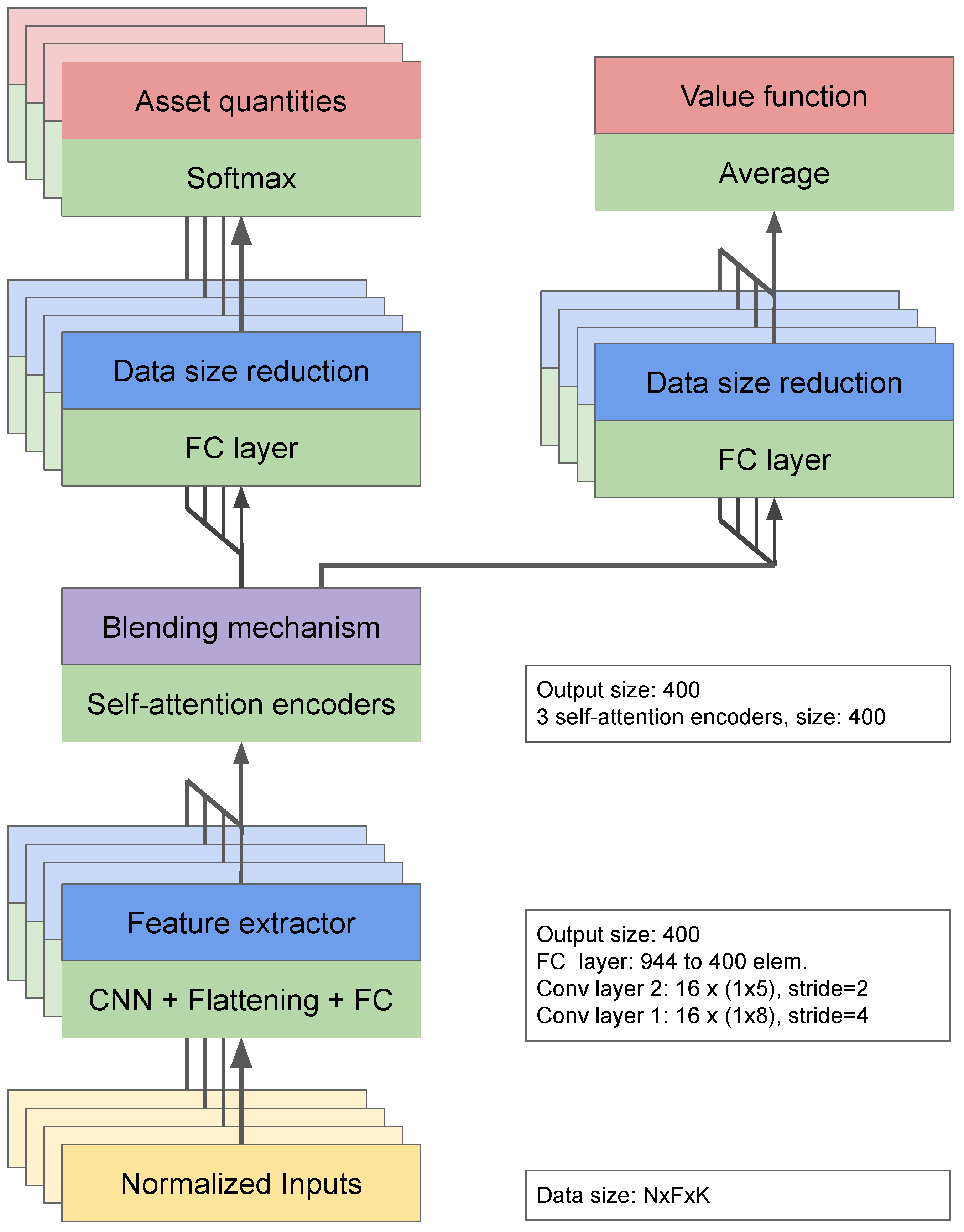
24] blend that information to produce the output. The components of our NN are shown in Figure 5. The data fed to the NN is an arrangement of financial indicators with dimensions F × N × K , where F is the number of financial indicators, N is the number of assets, and K is the number of past steps the agent is allowed to observe. The number of financial indicators equals six, as mentioned in Section 5.1. F is considered to be the number of channels of the input data. The number of assets in the dataset increases over time from 3 to 227 (see Table 2); therefore, N is not a constant. The number of past steps (K) depends on two factors: the number of days and sampling time. The data used in our experiments has a sampling time of 30 min, and the number of days our agent is allowed to observe is 20; therefore, K equals 960.
Since the channels of the data have a very different range of values, normalization was applied before feeding to the NN. The normalization consists of subtracting the mean from each channel and dividing the results by the standard deviation of the channel, resulting in a normal distribution with zero mean and unit standard deviation. Then, for each asset, the normalized inputs are independently passed through a sequence of two convolutional layers, which are the primal feature extraction mechanism of the NN. The extracted features are flattened and passed through a fully connected (FC) layer to produce a set of feature vectors. The feature vectors are directed one by one to the blending mechanism of the network, consisting of a set of three self-attention encoders [24].
The design of the self-attention encoders used in our NN is shown in Figure 6a. The self-attention encoders consist of two different sub-layers. The first sub-layer is a multi-head self-attention block, meaning it contains parallel feature extractors (heads), which generate independent feature vectors from the inputs. The number of heads in our self-attention blocks is eight. The distinct feature vectors generated by the heads are combined into a single feature vector using a linear layer, as shown in Figure 6b. Then, these results are fed to a normalization layer [25], which has a residual connection [25] to generate the output of the first sub-layer.
Each head in a self-attention encoder has three matrices: query ( W Q ), key ( W K ), and value ( W V ), which are the parameters to be trained. When a self-attention encoder receives the feature vectors corresponding to the assets, the feature vectors are concatenated and multiplied by the matrices W Q , W K , and W V to obtain the matrices Q, K and V, which are used to compute the output of the self-attention head using the Equation (1) of [24], which computes the amounts of attention having to be given to all the assets when generating the output of each asset.
The second sub-layer of the self-attention encoder also has two blocks. The first block is a feed-forward NN with two layers. The number of nodes in each layer is 400. The second block is a normalization layer with a residual connection, which produces the final output of the self-attention encoder. We use three identical self-attention encoders placed in sequential order as the blending mechanism of our design. The output of the blending mechanism is a high-level feature vector for each asset, containing information about every asset in the market. The generated feature vectors individually go through an FC layer to output a single scalar for each asset. These scalar values are normalized by a softmax layer to obtain the asset weights to be held in the next period.
We use an actor-critic design for the agent to learn an optimal policy that maximizes cumulative rewards. Therefore, the NN has two outputs: actor and critic. The actor determines which action to take and the critic evaluates how good the action was. The value function consists of another FC layer that takes the output of the self-attention layers and produces a scalar for each asset. Then, the output of the value function is simply the average of the scalar values.

5.3. Training

Our agent was trained using the ‘synchronous’ version of the Asynchronous Advantage Actor-Critic method (A3C) [26], introduced by Open AI, known as A2C. https://openai.com/blog/baselines-acktr-a2c/ (accessed on 2 August 2021). Therefore, the NN has two parts: actor and critic. The actor, also known as the policy, receives environment states and outputs actions. The critic, on the other hand, predicts the total reward the agent will receive at the end of the process by following the actions given by that specific policy. The policy is represented by π θ and the value function is represented by v θ . In our implementation, both the actor and critic are combined into a single NN with two independent output layers. Hence, they are trained simultaneously applying Adam optimizer [27] to the cost function shown in Equation (8), where s t is the state, a t is the action taken in that state, r t is the reward received, A is a variable named the advantage, and R is the total discounted reward (see [26]). The values of the parameters used in the optimization process are listed in Table 3. The values were chosen by comparing the performance of training sessions, which used hyperparameter values in the ranges shown in Table A1. We used 16 workers for data collection. Thus, in each iteration, we randomly draw 16 days from the training dataset to be the initial days of each trading session, and the workers execute trades for four days. Then, this data is used to compute the cost function, which in turn is used to improve both the policy and value function together.
L A 2 C ( θ ) = L π ( θ ) + η L v ( θ ) L π ( θ ) = E t = 0 T 1 log π θ ( a t | s t ) A ( s t , a t ) L v ( θ ) = E v π s t R t 2

5.4. Layer Analysis

In this subsection, we show how the information flows through the NN layers and give an interpretation of the meaning of the features computed by some of the layers of the NN. Recently, Makridakis et al. [28] made a critic about the performance of machine learning approaches on time-series forecasting tasks, which are closely related to our application. They state that ML researchers tend to over-utilize resources on tasks where simpler statistical methods can produce better results. Therefore, to show the relevance of each of the components of our NN, we fed our NN with the data of four popular cryptocurrencies drawn randomly from the dataset and analyzed the results computed by different layers.
The input layer of the NN is a normalization layer. The result of the normalization operation is shown in Figure 7. Both graphs are practically the same. However, an important difference is that, in the normalized data, most of the values corresponding to LINK are negative. This is useful as those values can be ruled out by the ReLU operation that takes place after the convolutional layers. Additionally, it has been shown that normalizing the inputs makes the training process faster and more stable [29].
The next group of layers is a series of convolutional layers. These layers have two functions: feature extraction and data size reduction. Figure 8 shows the features extracted by one of the convolutional masks of the first convolutional layer. As shown in the figure, this layer highlights assets that have significant positive changes in value, which is a typical convolution operation. We can see, as expected, that the features of the asset in green have been flattened out almost completely. These simple features are combined in deeper layers into abstract complex features which are given to the self-attention layers.
The final part is a sequence of self-attention layers, which choose the assets to be acquired in the subsequent step of the process. The results of the heads of the last self-attention layer are shown in Figure 9. The figure shows that most of the heads in the last layer focused their attention on Bitcoin, Ethereum, and Litecoin, which are the cryptocurrencies that increased the most their value in the tested sample. This shows that the layer can process the features extracted by the convolutional layers and determine the assets with higher chances to continue being in an increasing tendency.

6. Experiments

The experiments presented in this section evaluate the performance of the proposed NN architecture. These experiments are performed in an environment built using real data from a well-known cryptocurrency trading platform, allowing us to point out issues and make predictions about the performance of this system when implemented in a real market. The effects of including transactions fees in the training process are evaluated as well. We trained our model in an environment with transaction fees, and then we trained a clone of the model without fees. Next, both models were tested in the environment with transaction fees to observe the need of including the subprocess during the training stage. If a significant difference in performance cannot be observed during that experiment, this subprocess could be omitted in future training runs and only be used during deployment to save an important amount of time. We also validated the use of self-attention networks by comparing the performance of our design against a similar approach [22]. This architecture was also designed for markets with a large and non-constant number of assets, but it does not include self-attention networks in its design.
The agents are tested in multiple setups. In the first setup, each day in the test dataset was selected as an initial point, and each of the models performs a four-day trading session. The profits obtained by the models during the short experiments are recorded, and their average is taken as the overall performance. In the second setup, we run the agents throughout the test dataset in a single session (for 365 days), and the total profit is recorded as the overall performance. This allows us to analyze the robustness of the models to changes in the setup. Additionally, the algorithms were tested in the same setups of [22] and their performances were analyzed and compared. This includes a two-day trading period with transactions every 30 min, and a two-week trading period with transactions every six hours.

7. Results and Discussion

Performance of the Models

The performance of the tested models in the four-day experiment is listed in Table 4. Both networks using self-attention networks (SA-NET) introduced in this study outperform the baseline, showing the benefits of using self-attention networks to process data from a large pool of assets and extract high-level features. SA-NET must incur transaction fees during training, and it obtained average daily profits of 4.3%, while the model without fees (SA-NET-NF) obtained 3.4%. Therefore, the model trained in an environment with fees can make better decisions. However, the difference is not significant, meaning the most important factor to determine the performance of the two models is the self-attention networks.
In the setup with an episode length of two days, the results are similar among the competing algorithms. The algorithm that performed best is [22]. However, the difference with the respect to the rest of the tested algorithms is 0.1%. Additionally, the standard deviation of the experiments is large compare to the average performance. Therefore, we can conclude that the algorithms have similar performances when implemented in short trading episodes. These results are shown in Table 5. In the two-week setup, the results have a bigger spread. The algorithm that performed best in that setup is SA-NET. Again, the standard deviation of the performance is large. This is a characteristic of an extremely volatile market. However, the difference between the proposed approach and that of [22] is around 5%, showing that in longer episodes, the proposed NN outperforms the NN of our previous work. Figure 10a,b show examples of the performance of the tested algorithms in the two-day and two-week setup.
The results of the one-year setup, shown in Figure 10c, also demonstrate the self-attention design as the best alternative. However, despite obtaining a 5-fold return in one year, SA-NET is also the model suffering the worst losses during the run, which is evidence of taking riskier actions than the competing models. Nonetheless, the order of performance of the tested methods is consistent with both experiments. Therefore, the range of applicability of our system is flexible, showing the robustness of the presented approach.

8. Conclusions

We introduced a DRL system for cryptocurrency trading. Our system uses self-attention networks to simultaneously process data of a market with a large number of assets. Our deep NN has been trained using data from a real cryptocurrency market to execute daily trades. The experimental results show the methodology presented in this work outperforms the baseline, obtaining higher profits in two different setups, illustrating self-attention networks can extract meaningful relations from chaotic cryptocurrency data. We also studied the impact of transaction fees in cryptocurrency trading and presented three optimization solutions to deal with this important issue. The best solution has been integrating into the system to create a robust tool for cryptocurrency trading. Future work includes the optimization of the layers of the NN architecture to boost the performance and the application of the proposed system in stock markets and the FX market.

Author Contributions

Conceptualization, C.B.; methodology, C.B.; software, C.B.; validation, C.B.; formal analysis, C.B.; investigation, C.B.; data curation, C.B.; visualization, C.B.; draft preparation, C.B. and W.-H.C.; review and editing, C.B. and W.-H.C.; resources, W.-H.C.; supervision and proofreading, W.-H.C.; project administration, W.-H.C. Both authors have read and agreed to the published version of the manuscript.

Funding

This research received no external funding.

Institutional Review Board Statement

Not applicable.

Informed Consent Statement

Not applicable.

Conflicts of Interest

The authors declare no conflict of interest.

Abbreviations

The following abbreviations are used in this manuscript:
NNNeural network
RNNRecurrent neural network
RLReinforcement learning
RRLRecurrent reinforcement learning
GRUgated recurrent unit
SASelf-attention
IATInter-asset transactions
FXForeign exchange

Appendix A. Exchange Fee Minimization Algorithms

Note, Equation (2) contains a term τ i j k for all i and j, implying transactions among all assets are allowed. However, this is not always the case, and if extra constraints are imposed on the problem, it can be solved extremely efficiently. We impose extra constraints on the problem and build solutions for that case. Then, we remove those constraints and give the solution for the most general case.

Appendix A.1. No Inter-Asset Transactions

In some markets, exchanging shares between assets is not allowed. Instead, an investor needs to sell some shares to obtain cash, and use that cash to purchase shares of other assets. This is equivalent to the condition, τ i j k is zero if neither i nor j is zero. Applying this condition to Equations (2) and (4) results in Equations (A1) and (A2), respectively. We refer to this simplification of the fee minimization problem as ‘the constrained case’.
ρ k w i k + 1 = w i ˜ k ( 1 + f i 0 ) τ i 0 k + τ 0 i k , for i 0
ρ k = 1 i = 1 f i 0 τ i 0 k i = 1 f 0 i τ 0 i k
Note, an agent cannot buy and sell shares of the same asset at the same time. In other words, if τ i 0 k > 0 , then τ 0 i k = 0 , and if τ 0 i k > 0 , then τ i 0 k = 0 . These conditions can be explicitly written in terms of the ReLU function from Equation (A1), as shown in Equation (A3), where the ReLU function is denoted by ( . ) + .
( w ˜ i k ρ w i k + 1 ) + = ( 1 + f i 0 ) τ i 0 k ( ρ w i k + 1 w ˜ i k ) + = τ 0 i k
Next, Equation (A3) is substituted in Equation (A2) to obtain Equation (A4), where g i 0 represents the expression shown in Equation (A5).
ρ k = 1 i > 0 g i 0 ( w ˜ i k ρ k w i k + 1 ) + i > 0 f 0 i ( ρ k w i k + 1 w ˜ i k ) +
g i 0 = def f i 0 1 + f i 0
Then, the well-known identity of the ReLU function, shown in Equation (A6), is substituted into Equation (A4), and the terms in the resulting expression are rearranged, obtaining Equation (A7).
( a b ) + = ( b a ) + + ( a b )
ρ k = 1 i > 0 g i 0 + f 0 i w ˜ i k ρ k w i k + 1 + f 0 i w ˜ i k 1 + i > 0 f 0 i w i k + 1
Equation (A7) is used to iteratively search for the best possible ρ k , leading to the best possible values τ i 0 k and τ 0 i k for all i. The procedure is summarized in Algorithm 2. This algorithm is similar to the one given in Equation (2.6) of [30]. However, in their formulation, f i 0 and f 0 i are assumed to be constant for all i. Thus, the procedure in [30] is a special case of the proposed method. The proof of convergence of Algorithm 2 is given in Appendix B, where it is shown Algorithm 2 always converges to the optimal solution of the constrained case for the fee minimization problem when ρ 0 [ 0 , 1 ] .

Appendix A.2. The Solution for the General Case

The general solution for the fee minimization problem is computed using a linear program (LP). The solution is a generalization of the method presented in [22], which can solve the constrained case. The linear program is formulated using Equation (4) as the objective function and Equations (2) and (5) as constraints. However, Equation (A8) has to be modified because the objective variable ( ρ k ) appears explicitly in the expression. Therefore, substituting ρ k from Equation (4) and rearranging terms results in Equation (A8).
( 1 k j f k j τ k j k ) w i k + 1 + j ( 1 + f i j ) τ i j k j τ j i k = w ˜ i k for i { 0 , 1 , , N 1 }
This expression allows us to formulate the search for the solution of the general case of the fee minimization problem as an LP, as shown in Equation (A9). The LP in Equation (A9) is always feasible because the LP presented in [22] for the constrained case always has a feasible solution, and is a specific case of Equation (A9). Algorithm 3 summarizes the method to find the optimal solution for the fee minimization problem using Equation (A9). However, if the number of equality constraints, inequality constraints, or variables in an LP is large, the process to solve the LP can become impractically long, which is precisely the case for markets with a large number of assets. For this reason, we recommend using Equation (1) for IAT if the number of assets is large.
Maximize : ρ from Equation ( 4 ) Subject to : Equation ( 5 ) and Equation ( A8 )

Appendix B. Proof of the Absolute Convergence of Algorithm 2

In this section we prove Algorithm 2 always converges to the optimal solution for the constrained case of the fee minimization problem, i.e., no IAT are allowed or equivalently τ i j k = 0 if both i , j > 0 . Lemmas A1 to A6 are used to prove this fact. Lemma A1 justifies the use of Equation (A3) in Algorithm 2 and the other lemmas are used to prove the actual convergence of the algorithm. Theorem A1 combines the most important results of these lemmas. During the rest of the proof, the terms ‘problem’ and ‘optimal solution’ refer to those of this particular case. This proof is similar to the one given by Jiang et al. [31] for the constrained case in which τ 0 i k and τ i 0 k are fixed values for i { 1 , 2 , , N 1 } . However, our proof is more general since no fixed values are assumed for τ i 0 k and τ 0 i k , and it is also less restrictive since we do not require the values of fees to be less than 0.38.
Lemma A1.
An optimal solution cannot have both, τ i 0 k > 0 and τ 0 i k > 0 for any i { 1 , 2 , , N 1 } .
Proof. 
This fact is proven by contradiction, showing there is always a solution with a larger ρ k that can be constructed from another solution that has both τ i 0 k and τ i 0 k larger than 0 for some index i = κ . Let us denote the optimal values for the problem as ρ * k , τ 0 i * k and τ i 0 * k for i { 1 , 2 , , N 1 } . Assume the optimal solution has at least one asset κ such that τ κ 0 * and τ 0 κ * are both larger than 0. Assume also without loss of generality (WLOG) w κ k + 1 > 0 since otherwise τ 0 κ * would be exactly zero, as is implied by Equation (5). Then, we can rewrite Equation (2) for the optimal solution as shown in Equation (A10), where also the fact τ i j k = 0 if both i , j > 0 was used.
ρ * k w i k + 1 = w i ˜ k ( 1 + f i 0 ) τ i 0 * k + τ 0 i * k for i { 1 , 2 , , N 1 }
Since the solution is optimal, it has to satisfy Equation (A11).
ρ * k ρ k , for all ρ k
Then, for the asset k we can define the variables τ κ 0 k and τ 0 κ k as follows. If ( 1 + f k 0 ) τ κ 0 * k + τ 0 κ * k 0 , τ κ 0 k = def τ κ 0 * k τ 0 κ * k / ( 1 + f κ 0 ) and τ 0 κ k = def 0 , otherwise τ κ 0 k = def 0 and τ 0 κ k = def ( 1 + f κ 0 ) τ κ 0 * k + τ 0 κ * k . Substituting τ κ 0 * k and τ 0 κ * k by these new variables into Equation (A10) gives Equation (A12).
ρ * k w κ k + 1 = w ˜ κ k ( 1 + f κ 0 ) τ κ 0 k + τ 0 κ k
Note, both τ k 0 k and τ 0 k k are smaller than τ k 0 * k and τ 0 k * k , respectively; in fact, one of them has to be zero. The difference between the loss due to the ‘stared’ variables and the ‘primed’ variables is given in Equation (A13).
D = def f κ 0 τ κ 0 * k + f 0 κ τ 0 κ * k f κ 0 τ κ 0 k f 0 κ τ 0 κ k
By substituting the primed variables by the stared variables, the value corresponding the the asset 0 increases an amount corresponding to the value of D (see Equation (A13)). Therefore, the desired weights after the transactions are no longer satisfied since w 0 k + 1 becomes larger while the rest w i k + 1 remain the same. To fix this problem, the value of D is distributed among all assets. For this purpose the variables τ 0 i * k for all i κ are substituted by τ ^ 0 i k using Equation (A14); similarly, τ 0 κ k is substituted by τ ^ 0 κ k using Equation (A15). The new variables Δ τ 0 i k used in Equations (A14) and (A15) are defined in Equation (A16). This definition for the variables Δ τ 0 i k ensures all Δ τ 0 i k are proportional to their corresponding w i k + 1 and also ensures the relation i ( 1 + f 0 i ) Δ τ 0 i k = D is satisfied. Therefore, the variables τ ^ 0 i k correspond to a feasible solution to the problem since all desired weights are satisfied again. The next step is to prove the discount rate corresponding to this solution, named ρ ^ k , is larger than ρ * k .
τ ^ 0 i k = def τ 0 i * k + Δ τ 0 i k , i κ
τ ^ 0 κ k = def τ 0 κ k + Δ τ 0 κ
Δ τ 0 i k = def D w i k + 1 j ( 1 + f 0 j ) w j k + 1
Replacing τ ^ 0 k k from Equation (A15) for τ 0 k k in Equation (A12) results in Equation (A17), which corresponds to the equation for the asset κ for the constructed solution. By simplifying this expression, we arrive to a relation between ρ ^ k and ρ * k .
ρ ^ k w k k + 1 = w ˜ κ k ( 1 + f κ 0 ) τ κ 0 k + τ ^ 0 κ k = w ˜ κ k ( 1 + f κ 0 ) τ κ 0 k + τ 0 κ k + Δ τ 0 κ k = ρ * k w k k + 1 + D w κ k + 1 j ( 1 + f 0 j ) w j k + 1 = ρ * k 1 + D j ( 1 + f 0 j ) w j k + 1 w κ k + 1 ρ ^ k = ρ * k 1 + D j ( 1 + f 0 j ) w j k + 1
The fact w κ k > 0 was used to simplify that variable from both sides of Equation (A17). Note, Equation (A17) implies ρ ^ k > ρ * k , which contradicts Equation (A11). Therefore, the assumption that exists an optimal solution such that both τ i 0 k and τ 0 i k are positive for some index i = κ is false. This concludes the proof of Lemma A1. □
Let us define the function f ( ρ ) using the right-hand side (RHS) of Equation (A7) as shown in Equation (A18). Note, Equation (2) consist of computing f ( ρ ) , assign that value to ρ and repeat the process over and over until ρ converges. The following lemmas are properties of the function f ( ρ ) and the consequences of this iterative process.
f ( ρ ) = def 1 i > 0 g i 0 + f 0 i w ˜ i k ρ w i k + 1 + f 0 i w ˜ i k 1 + i > 0 f 0 i w i k + 1
Lemma A2.
The function f ( ρ ) (see Equation (A18)) increases monotonically, i.e., ρ 1 > ρ 1 f ( ρ 1 ) f ( ρ 2 ) . Furthermore, f ( ρ ) is a concave function.
Proof. 
Note, the expression w ˜ i k ρ w i k + 1 + on the RHS of Equation (A18) is a convex, monotonically decreasing function of ρ for all i. Then, the expression
i > 0 g i 0 + f 0 i w ˜ i k ρ w i k + 1 + is also convex and monotonically decreasing since it is just a weighted summation of convex, monotonically decreasing functions with positive scaling weights g i 0 + f 0 i . However, the summation has a negative sign at the front, changing the expression into a concave, monotonically increasing function instead. The rest of elements on the RHS of Equation (A18) are simply constants that translate the expression on the plane formed by ρ and f ( ρ ) , but do not change its concave and monotonically increasing nature. □
Lemma A3.
f ( 0 ) > 0 .
Proof. 
Substituting 0 for ρ in Equation (A18) results in Equation (A19).
f ( 0 ) = 1 i > 0 ( g i 0 + f 0 i ) w ˜ i k f 0 i w ˜ i k 1 + i > 0 f 0 i w i k + 1 = 1 i > 0 g i 0 w ˜ i k 1 + i > 0 f 0 i w i k + 1
Note, Equation (A19) implies f ( 0 ) cannot be negative or zero because both numerator and denominator are always positive. It is obvious that the denominator is positive since each part of the expression is positive. The numerator, on the other hand has negative expressions; therefore, it has to be analyzed carefully. Note, The definition of g i 0 (see Equation (A5)) implies g i 0 < 1 for all i and i w ˜ i k = 1 ; thus, i g i 0 w ˜ i k < 1 , which implies the numerator is positive. □
Lemma A4.
f ( 1 ) 1 .
Proof. 
This fact is proven by contradiction as follows. Assume f ( 1 ) > 1 . Then, substituting 1 for ρ in Equation (A18) gives Equation (A20).
f ( 1 ) = 1 i > 0 g i 0 + f 0 i w ˜ i k w i k + 1 + f 0 i w ˜ i k 1 + i > 0 f 0 i w i k + 1 > 1 i > 0 g i 0 + f 0 i w ˜ i k w i k + 1 + f 0 i w ˜ i k > i > 0 f 0 i w i k + 1
Then, using Equation (A6) in Equation (A20) gives Equation (A21).
i > 0 ( g i 0 + f 0 i ) w i k + 1 w ˜ i k + + w ˜ i k w i k + 1 f 0 i w ˜ i k > i > 0 f 0 i w i k + 1 i > 0 ( g i 0 + f 0 i ) w i k + 1 w ˜ i k + + g i 0 w ˜ i k w i k + 1 > 0 i > 0 g i 0 w i k + 1 w ˜ i k > i > 0 ( g i 0 + f 0 i ) w i k + 1 w ˜ i k + i > 0 g i 0 w i k + 1 w ˜ i k > i > 0 g i 0 w i k + 1 w ˜ i k +
And Equation (A21) is clearly a contradiction since w i k + 1 w ˜ i k w i k + 1 w ˜ i k + for any asset i. □
Lemma A5.
The function f ( ρ ) defined in Equation (A18) cannot have more than one fixed-point ( f ( ρ ) = ρ ) in the interval [ 0 , 1 ] .
Proof. 
This fact is proven by contradiction as follows. Assume f ( ρ ) has at least two different fixed-points in the interval [ 0 , 1 ] , namely ρ 1 and ρ 2 . Assume WLOG ρ 1 < ρ 2 . Then, using the definition of fixed-point, we can write Equation (A22). And using the fact that f ( ρ ) is concave and the definition of concave function, which can be found in the work of Boyd and Vandenberghe [32], we can write Equation (A23), where x 1 and x 2 are any elements in the domain of the function and θ is any value in the interval [ 0 , 1 ] .
f ( ρ 1 ) = ρ 1 , f ( ρ 2 ) = ρ 2
f ( θ x 1 + ( 1 θ ) x 2 ) θ f ( x 1 ) + ( 1 θ ) f ( x 2 ) , 0 θ 1
Next, substituting x 1 and x 2 by 0 and ρ 2 , respectively in Equation (A23) results in Equation (A24).
f ( θ 0 + ( 1 θ ) ρ 2 ) θ f ( 0 ) + ( 1 θ ) f ( ρ 2 )
Note, since ρ 1 < ρ 2 , we can define θ ^ as the solution of equation ρ 1 = θ ^ 0 + ( 1 θ ^ ) ρ 2 , which always gives a value in the interval [ 0 , 1 ) . Then, substituting this expression in Equation (A22) for ρ 1 gives Equation (A25).
f ( θ ^ 0 + ( 1 θ ^ ) ρ 2 ) = θ ^ 0 + ( 1 θ ^ ) ρ 2
And substituting Equation (A22) for ρ 2 in Equation (A25) gives Equation (A26).
f ( θ ^ 0 + ( 1 θ ^ ) ρ 2 ) = θ ^ 0 + ( 1 θ ^ ) f ( ρ 2 )
Finally, substituting zero for f ( 0 ) in Equation (A26) by Equation (A3) results in the inequality shown in Equation (A27).
f ( θ ^ 0 + ( 1 θ ^ ) ρ 2 ) < θ ^ f ( 0 ) + ( 1 θ ^ ) f ( ρ 2 )
But, Equation (A27) contradicts Equation (A24). Therefore, the assumption that f ( ρ ) has more than one fixed-point is false. □
Note, we have not proved that there exists a fixed-point for f in the interval [ 0 , 1 ] , but only proved there cannot be more than one. In fact, there is always a single fixed-point for f in that interval as proven in Lemma A6.
Lemma A6.
The sequences { ρ k } 0 , where ρ 0 [ 0 , 1 ] and ρ k = f ( ρ k 1 ) for k > 0 , with f ( ρ ) defined by Equation (A18), monotonically converge to the only fixed-point of f in the interval [ 0 , 1 ] .
Proof. 
If the first element of the sequence ρ 0 is chosen to be in the interval [ 0 , 1 ] , then by Lemmas A2 to A4, the next element of the sequence x 1 falls in the interval ( 0 , 1 ] . These lemmas impose hard limits for f in the interval [ 0 , 1 ] , namely 0 < f ( 0 ) f ( ρ ) f ( 1 ) 1 . Using this fact we prove the monotonicity of the sequence by induction. Assume that ρ k ρ k 1 . Then by Lemma A2 we obtain Equation (A28).
ρ k ρ k 1 f ( ρ k ) f ( ρ k 1 )
And applying the definition of the sequence to Equation (A28) results in Equation (A29).
ρ k + 1 = f ( ρ k ) f ( ρ k 1 ) = ρ k ρ k + 1 ρ k
Therefore, if ρ 1 ρ 0 , the whole sequence is monotonically increasing. Following a similar argument, we can also show if ρ 1 ρ 0 , the sequence decreases monotonically. Then, the base step of the induction is determined by the outcome of f ( ρ 0 ) . Therefore, since the sequence is monotonic and bounded above and below, the Monotone Convergence Theorem [33] implies all sequences defined in Lemma A6 must converge. This fact is summarized in Equation (A30) for any ρ 0 in the interval [ 0 , 1 ] .
lim k ρ k + 1 = ρ k f ( ρ k ) = ρ k as k
Finally, using Lemma A5 we conclude that all sequences defined in Lemma A6 can only converge to a unique value. □
Theorem A1.
The solution returned by Algorithm 2 is optimal.
Proof. 
Lemma A1 gives a necessary (but not sufficient) condition for any optimal solution, namely the solution has to satisfy the constraints given in Equation (A3). Additionally, if there is an optimal solution, it has to be a fixed-point of Equation (A18). Lemma A6 shows the output of Algorithm 2 is the unique fixed-point of f in the interval ( 0 , 1 ] . And since any optimal solution has to be a fixed-point of f, we conclude that the solution given by Algorithm 2 is the optimal solution. □

Appendix C. Fine Tuning Parameters

Table A1. Fine tuning parameters.
ParameterRangeIncrement
# of optimization steps100,000–200,00010,000
Learning rate ( α )1 × 10 7 –1 × 10 6 1 × 10 7
A2C parameter ( η )0.1–0.70.1
# of masks in CNN layers8–328
# of SA layers1–81
# of heads SA layers8–328

References

  1. Berentsen, A.; Schär, F. Stablecoins: The quest for a low-volatility cryptocurrency. In The Economics of Fintech and Digital Currencies; CEPR Press: London, UK, 2019; pp. 65–75. [Google Scholar]
  2. Wu, X.; Chen, H.; Wang, J.; Troiano, L.; Loia, V.; Fujita, H. Adaptive stock trading strategies with deep reinforcement learning methods. Inf. Sci. 2020, 538, 142–158. [Google Scholar] [CrossRef]
  3. Moody, J.; Wu, L.; Liao, Y.; Saffell, M. Performance functions and reinforcement learning for trading systems and portfolios. J. Forecast. 1998, 17, 441–470. [Google Scholar] [CrossRef]
  4. Moody, J.; Saffell, M. Learning to trade via direct reinforcement. IEEE Trans. Neural Net. 2001, 12, 875–889. [Google Scholar] [CrossRef] [PubMed] [Green Version]
  5. Gold, C. FX trading via recurrent reinforcement learning. In Proceedings of the 2003 IEEE International Conference on Computational Intelligence for Financial Engineering, Hong Kong, China, 20–23 March 2003; pp. 363–370. [Google Scholar]
  6. Dempster, M.; Leemans, V. An automated FX trading system using adaptive reinforcement learning. Expert Syst. Appl. 2006, 30, 543–552. [Google Scholar] [CrossRef]
  7. Maringer, D.; Ramtohul, T. Threshold recurrent reinforcement learning model for automated trading. In European Conference on the Applications of Evolutionary Computation; Springer: Berlin/Heidelberg, Germany, 2010; pp. 212–221. [Google Scholar]
  8. Zhang, J.; Maringer, D. Indicator selection for daily equity trading with recurrent reinforcement learning. In Proceedings of the 15th Annual Conference Companion on Genetic and Evolutionary Computation, Amsterdam, The Netherlands, 6–10 July 2013; pp. 1757–1758. [Google Scholar]
  9. Mnih, V.; Kavukcuoglu, K.; Silver, D.; Graves, A.; Antonoglou, I.; Wierstra, D.; Riedmiller, M. Playing atari with deep reinforcement learning. arXiv 2013, arXiv:1312.5602. [Google Scholar]
  10. Deng, Y.; Bao, F.; Kong, Y.; Ren, Z.; Dai, Q. Deep direct reinforcement learning for financial signal representation and trading. IEEE Trans. Neural Net. Learn. Syst. 2016, 28, 653–664. [Google Scholar] [CrossRef]
  11. Jiang, Z.; Liang, J. Cryptocurrency portfolio management with deep reinforcement learning. In Proceedings of the 2017 Intelligent Systems Conference (IntelliSys), London, UK, 7–8 September 2017; pp. 905–913. [Google Scholar]
  12. Bu, S.J.; Cho, S.B. Learning optimal Q-function using deep Boltzmann machine for reliable trading of cryptocurrency. In Proceedings of the International Conference on Intelligent Data Engineering and Automated Learning, Madrid, Spain, 21–23 November 2018; pp. 468–480. [Google Scholar]
  13. Pendharkar, P.C.; Cusatis, P. Trading financial indices with reinforcement learning agents. Expert Syst. Appl. 2018, 103, 1–13. [Google Scholar] [CrossRef]
  14. Liang, Z.; Chen, H.; Zhu, J.; Jiang, K.; Li, Y. Adversarial deep reinforcement learning in portfolio management. arXiv 2018, arXiv:1808.09940. [Google Scholar]
  15. Jeong, G.; Kim, H.Y. Improving financial trading decisions using deep Q-learning: Predicting the number of shares, action strategies, and transfer learning. Expert Syst. Appl. 2019, 117, 125–138. [Google Scholar] [CrossRef]
  16. Chung, J.; Gulcehre, C.; Cho, K.; Bengio, Y. Empirical evaluation of gated recurrent neural networks on sequence modeling. arXiv 2014, arXiv:1412.3555. [Google Scholar]
  17. Luo, B.; Liu, D.; Wu, H.N.; Wang, D.; Lewis, F.L. Policy gradient adaptive dynamic programming for data-based optimal control. IEEE Trans. Cybern. 2016, 47, 3341–3354. [Google Scholar] [CrossRef] [PubMed]
  18. Aboussalah, A.M.; Lee, C.G. Continuous control with stacked deep dynamic recurrent reinforcement learning for portfolio optimization. Expert Syst. Appl. 2020, 140, 112891. [Google Scholar] [CrossRef]
  19. Park, H.; Sim, M.K.; Choi, D.G. An intelligent financial portfolio trading strategy using deep Q-learning. Expert Syst. Appl. 2020, 158, 113573. [Google Scholar] [CrossRef]
  20. Hochreiter, S.; Schmidhuber, J. Long-short-term memory. Neural Comput. 1997, 9, 1735–1780. [Google Scholar] [CrossRef]
  21. Lei, K.; Zhang, B.; Li, Y.; Yang, M.; Shen, Y. Time-driven feature-aware jointly deep reinforcement learning for financial signal representation and algorithmic trading. Expert Syst. Appl. 2020, 140, 112872. [Google Scholar] [CrossRef]
  22. Betancourt, C.; Chen, W.H. Deep reinforcement learning for portfolio management of markets with a dynamic number of assets. Expert Syst. Appl. 2021, 164, 114002. [Google Scholar] [CrossRef]
  23. Papadimitriou, C.H.; Steiglitz, K. Combinatorial Optimization: Algorithms and Complexity; Courier Corporation: North Chelmsford, MA, USA, 1998. [Google Scholar]
  24. Vaswani, A.; Shazeer, N.; Parmar, N.; Uszkoreit, J.; Jones, L.; Gomez, A.N.; Kaiser, L.; Polosukhin, I. Attention is all you need. arXiv 2017, arXiv:1706.03762. [Google Scholar]
  25. He, K.; Zhang, X.; Ren, S.; Sun, J. Deep residual learning for image recognition. In Proceedings of the IEEE Conference on Computer Vision and Pattern Recognition, Las Vegas, NV, USA, 27–30 June 2016; pp. 770–778. [Google Scholar]
  26. Mnih, V.; Badia, A.P.; Mirza, M.; Graves, A.; Lillicrap, T.; Harley, T.; Silver, D.; Kavukcuoglu, K. Asynchronous methods for deep reinforcement learning. In Proceedings of the International Conference on Machine Learning; PMLR: New York, NY, USA, 2016; pp. 1928–1937. [Google Scholar]
  27. Kingma, D.P.; Ba, J. Adam: A method for stochastic optimization. arXiv 2014, arXiv:1412.6980. [Google Scholar]
  28. Makridakis, S.; Spiliotis, E.; Assimakopoulos, V. Statistical and Machine Learning forecasting methods: Concerns and ways forward. PLoS ONE 2018, 13, e0194889. [Google Scholar] [CrossRef] [PubMed] [Green Version]
  29. Ba, J.L.; Kiros, J.R.; Hinton, G.E. Layer normalization. arXiv 2016, arXiv:1607.06450. [Google Scholar]
  30. Ormos, M.; Urbán, A. Performance analysis of log-optimal portfolio strategies with transaction costs. Quant. Financ. 2013, 13, 1587–1597. [Google Scholar] [CrossRef]
  31. Jiang, Z.; Xu, D.; Liang, J. A deep reinforcement learning framework for the financial portfolio management problem. arXiv 2017, arXiv:1706.10059. [Google Scholar]
  32. Boyd, S.; Vandenberghe, L. Convex Optimization; Cambridge University Press: Cambridge, UK, 2004. [Google Scholar]
  33. Rudin, W. Principles of Mathematical Analysis; McGraw-Hill: New York, NY, USA, 1964; Volume 3. [Google Scholar]
Figure 1. Block diagram of the trading process.
Applsci 11 07377 g001
Figure 2. Computation time vs. number of assets for the fee minimization algorithms. The center lines represent averages on 1000 tests for each algorithm. The borders of the shaded areas represent the maximum and minimum values. The computation time in the y-axis is in logarithmic scale. NO-IAT stands for ‘without IAT’.
Applsci 11 07377 g002
Figure 3. Graph of the error of Algorithm 2 and BCH-21 with respect to the number of assets in the market. The center lines represent the average on 1000 thousand tests. The inner shaded area represents the standard deviation around the average. The borders of the outer shaded area represent the maximum and minimum values.
Applsci 11 07377 g003
Figure 4. Graph of the error of Algorithm 1 with respect to the number of assets in the market. The center lines represent the average on 1000 thousand tests. The inner shaded area represents the standard deviation around the average. The borders of the outer shaded area represent the maximum and minimum values.
Applsci 11 07377 g004
Figure 5. Self-attention network diagram for cryptocurrency trading. The activation function of all FC layers is the ReLU function. The output size of the final FC layers is one.
Applsci 11 07377 g005
Figure 6. Self-attention architecture and multi-head attention architecture.
Applsci 11 07377 g006
Figure 7. Raw data vs. normalized data.
Applsci 11 07377 g007
Figure 8. Values extracted by a convolutional layer.
Applsci 11 07377 g008
Figure 9. Attention values of a self-attention layer.
Applsci 11 07377 g009
Figure 10. Performance of three competing algorithms in trading episodes with different lenghts.
Applsci 11 07377 g010
Table 1. Literature review summary.
WorkYearMain Contributions
Moody et al. [3]1998Proposed the RRL method.
Moody and Saffel [4]2001Expanded RRL and compared to other
approaches.
Gold [5]2003Applied RRL to the FX market.
Dempster and Leemans [6]2006Proposed an adaptive reinforcement
method for trading in the FX market.
Maringer and Ramtohul [7]2010Proposed a threshold RRL method.
Zhang and Maringer [8]2013Combined RRL with a technical and
fundamental analysis for stock trading.
Deng et al. [10]2016Combined fuzzy logic and RNNs for
stock trading.
Jiang and Liang [11]2017Trained CNNs using Policy Gradient
for cryptocurrency trading.
Bu and Cho [12]2018Used RNNs and Boltzmann machines
for cryptocurrency trading.
Pendharkar and Cusatis [13]2018Compared the performance of
multiple DRL techniques for stock
market trading.
Liang et al. [14]2018Proposed an adversarial training
method to enhance DRL methods.
Jeong and Kim [15]2019Used Q-learning and transfer learning
for stock trading.
Wu et al. [2]2020Used GRUs for stock market trading.
Aboussalah and Lee [18]2020Proposed the method SDDRL for
stock market trading.
Park et al. [19]2020Trained an LSTM network using
Q-learning for stock market trading.
Lei et al. [21]2020Trained a GRU network using Policy
Gradient for stock market trading.
Betancourt and Chen [22]2021Proposed a NN architecture for markets
with a dynamic number of assets.
Table 2. Dataset properties.
FeatureValue
Initial date17 August 2017
Final date3 November 2020
# of days (training)809
# of days (test)365
# of assets3 to 227
# of indicators9
Sampling time30 min
# of entries (training)38,832
# of entries (test)17,520
Fees (except BNB)0.1%
Fees BNB0.05%
Table 3. List of training parameters.
ParameterValue
# of workers16
# of step per episode4
# of step per rollout4
# of optimization steps150,000
Learning rate ( α )7 × 10 7
Adam opt. param. ( β 1 )0.9
Adam opt. param. ( β 2 )0.999
Decay factor ( γ )0.99
A2C parameter ( η )0.5
Advantage parameter ( λ )0.95
Table 4. Comparison of the performance of the algorithms in a short and long trading episode.
ModelFour-Day EpisodeOne-Year Episode
MeanStandard
Deviation
Total Profit
SA-NET0.0430.114.66
SA-NET-NF0.0340.103.80
Betancourt and Chen [22]0.0300.072.24
Table 5. Comparison of the performance of the algorithms in the two-day and two-week trading episode.
ModelTwo-Day EpisodeTwo-Week Episode
MeanStandard
Deviation
MeanStandard
Deviation
SA-NET0.0280.070.330.30
SA-NET-NF0.0270.060.310.26
Betancourt and Chen [22]0.0290.060.280.33
Publisher’s Note: MDPI stays neutral with regard to jurisdictional claims in published maps and institutional affiliations.

