Article

Three-Dimensional Imaging of Metallic Grain by Stacking the Microscopic Images

1
IT-Based Real-Time NDT Center, Chosun University, Gwangju 61452, Korea
2
Department of Electronics Engineering, Chosun University, Gwangju 61452, Korea
3
Interdisciplinary Program in IT-Bio Convergence System, Chosun University, Gwangju 61452, Korea
4
Daegyeong Regional Division, Korea Institute of Industrial Technology, Daegu 42990, Korea
*
Author to whom correspondence should be addressed.
Appl. Sci. 2021, 11(17), 7787; https://doi.org/10.3390/app11177787
Submission received: 20 July 2021 / Revised: 20 August 2021 / Accepted: 23 August 2021 / Published: 24 August 2021
(This article belongs to the Special Issue Novel Approaches for Nondestructive Testing and Evaluation)

Abstract

:
Three-dimensional observation of metal grains (MG) has a wide potential application serving the interdisciplinary community. It can be used for industrial applications and basic research to overcome the limitations of non-destructive testing methods, such as ultrasonic testing, magnetic particle testing, and eddy current testing. This study proposes a method and its implementation algorithm to observe (MG) metal grains in three dimensions in a general laboratory environment equipped with a polishing machine and a metal microscope. An image was taken by a metal microscope while polishing the mounted object to be measured. Then, the metal grains (MGs) were reconstructed into three dimensions through local positioning, binarization, boundary extraction, (MG) selection, and stacking. The goal is to reconstruct the 3D MG in a virtual form that reflects the real shape of the MG. The usefulness of the proposed method was verified using the carbon steel (SA106) specimen.

1. Introduction

Predicting, comprehending, and monitoring the microstructure and mechanical properties, such as heterogeneous microstructure, ductility decreases, the concentration of residual stress, brittleness, and deterioration of toughness, of critical structures, such as heat exchangers, power plants, the oil and gas industry, chemical engineering, and especially nuclear power plants, is important to ensure safety and avoid failures that can lead to environmental disasters, causalities, and financial losses. To prevent and avert such risks, and to ensure the continued safety and integrity of these structures, periodic inspections are required [1,2,3,4].
Numerous non-destructive methods can be used for microstructure characterization. In most cases, non-destructive testing cannot directly determine material characteristics, which are established by destructive testing. To quantify material properties non-destructively, non-destructive methods must be correlated with destructively measured standard data. The limitation and disadvantage of destructive methods are that they do not allow the characterization of the evolution of material properties of the same specimen when successively damaged [3], and they are not easily applicable to characterize the mechanical behavior of materials, if possible, with restricted, difficult and expensive access, even using a numerical simulation, such as the finite element method.
The finite element method is used to analyze the relationship between the load, stress-strain, and resistance to failure of a structure [5,6,7,8]. Meanwhile, according to conventional studies, the size and shape of the microstructure affect the strength, toughness, and creep resistance of the structure [9,10,11]. However, it is not easy to reflect and demonstrate this with the finite element method [12,13,14,15]. This is because the factor used in the finite element method is the shape of the structure and does not include the microstructure of the structure itself. Therefore, we have not yet seen an example in which the size of the microstructure is inserted as an analysis condition in the finite element method (or two-dimensional analysis). Therefore, in order to analyze the shape and size of the microstructure, it is necessary to express the shape of the grain in three dimensions. On the other hand, the size and shape of the grains affect the analysis results of non-destructive tests [16,17,18,19], such as ultrasonic testing, magnetic particle testing, and eddy current testing. For instance, in the case of ultrasonic examination, research results have been reported that the size and shape of the microstructure influence the scattering of the sound [20]. However, analysis or qualitative matters considering only the average size of the microstructure are reported in [21], and it is difficult to find previous studies on ultrasound wave scattering targeting the size and shape of the actual microstructure. In the magnetic particle inspection method, the sample is magnetized, and the adsorption of magnetic particles by the magnetic flux leakage generated around the defect is observed. At this point, if a strong external magnetic field is applied and then removed, residual magnetization occurs. A similar fault signal is generated, in which magnetic particles are adsorbed even in non-defective areas due to residual magnetization [22,23,24]. Even though the deformation caused by an external force causes the magnetic moment inside the magnetic domain to be anisotropic in a specific direction and, therefore, residual magnetization occurs even if an external magnetic field is not applied [25,26,27]. In addition, residual magnetization is frequently generated in welds where heat and residual stress are generated by an external force. In the eddy current method of inspection, an induced current is applied to an object to be measured, and the distortion of the induced current occurring around a fault, that is, a change in impedance and a different phase due to eddy currents is measured [28,29]. However, it is difficult to determine the presence or size of a defect due to the edge effect that occurs at the end of the object to be measured [30]. This means that even when the grain is needle-shaped or the shape changes rapidly, the eddy current signal can be affected. It is important to provide a means of quantitatively measuring and expressing the three-dimensional shape of a grain in order to grasp the effects of such effects, i.e., the formation of magnetic domains, residual magnetization, and the effects of edge according to the shape and size of the grain. According to nano-radiography and tomography, the metal grain can be imaged in three dimensions [31,32]. Nevertheless, this requires very high accuracy and expensive equipment, including X-ray shielding. Furthermore, it is difficult to measure the distribution of magnetic domains within the grain in three dimensions. In addition, under the heat treatment influence, the application of external field and mechanical stress can rearrange the martensite variant and can change the magnetic domains. It is important to understand their effect not only at the macroscopic level but also at the microscopic level [33,34,35,36]. In this context, the use of an alternative method to overcome the limitations of non-destructive testing (NDT) techniques can make a valuable contribution to the characterization of materials and the evaluation of microstructure performance through rapid and efficient experiments and simulations. In this paper, we present a method to reproduce the real shape and size of the grains of the tested sample SA106 by pilling up two-dimensional images obtained by a metal microscope. To achieve this target, we introduce fixtures, procedures, and software algorithms based on mathematical formulas.
Several studies have previously developed 2D and 3D techniques to construct a way to study microstructure using different experimental and simulation techniques. The results of these studies lead to a good outcome that provides access to crucial structural information of the investigated materials, which facilitates and enhances the understanding of physical and chemical concepts at the microscopic level [37,38,39,40,41,42,43].
However, we have not seen any work similar to our work, which allows the reconstruction, extraction, and selection of one or more grains with the exact shape and size of the inspected material, without using extensive software and hardware, but just simple equipment and some algorithms. It should be emphasized that the method presented here permits: (1) 3D grain shape obtaining; (2) using conventional research laboratory environment; (3) easy preparing specimens; (4) multi-parallel data acquisition; (5) easy 3D image processing. This is particularly important for the industry and research laboratories.
The finding is encouraging for the near future application of the method for the analysis of 3D stress, strain deformation at grain level, and the analytical study of non-destructive evaluations using electromagnetic and ultrasound testing.

2. Specimen and Layer Capture

In this study, carbon steel SA106 was targeted. The sample was cut and cropped to a small volume of 25 × 9 × 25 mm (width × length × height), respectively, and mounted on a cylindrical resin with a diameter of 35 mm and a height of 27 mm. Then, the observation side and the backside of the mounted specimen were polished to be exposed outside the resin. This allows the “polished” height to be measured more accurately when viewed under a microscope. In other words, when measuring the height of the sample with a micrometer after polishing, errors likely to be caused by compression of the resin can be avoided when the resin is used as a measurement reference and not the surface of the sample. As shown in Figure 1a, the side surface was polished to deflect by 1.84 mm. This deflected side surface (hereafter “key-hole”) was used as a reference surface for microscopic observation. Figure 1b is a jig for uniform grinding of the key-hole, and Figure 1c is a template (state) in which the key-hole is polished in the sample mounted in the jig. Figure 1d illustrates these mounted samples; they are inserted into the X-Y stage holder under the microscope and are fixed by a key (expressed in black in the figure). Due to this structure, the area observed by the microscope can fix the measurement surface with a repeatability of the order of 10 to 20 μm.
The observation surface was polished using SiC polishing pads FEPA P200, P400, P800, P1200, and P2000. The last stage, P2000, has a grid size of 10.3 μm. Finally, fine polishing was carried out for 20 s using polishing cloths and polycrystalline diamond paste having a grid size of 1 μm. Once the micro-polishing was completed, an etchant solution obtained by diluting with nitric acid 3 g in 65 g ethanol was exposed onto the observation surface for 5 s, followed by ultrasonic cleaning with distilled water for 15 s and then cleaning with ethanol for 10 s. This chemical etching was performed a total of three times. The height of the four sides of the test sample was measured with a micrometer having an accuracy of ±0.01 μm, visualized through the microscope (500×), and recorded on the laptop. The observation by the microscope was repeated while repeating fine polishing, chemical etching, as well as the height measurement and can be directly linked to the 3D image processing. A total of 60 fine polishes were performed; Table 1 shows the heights measured in each layer.

3. Algorithms for 3D Imaging of Grains and Results

3.1. Local Positioning

As mentioned above, the main goal of this study is to image MG in 3D. To reach our purpose, micrographs are taken while repeatedly polishing. At this time, the height information measured by the micrometer is taken as the z-axis. Then the location of the boundary of a specific MG selected in the photo is stored as the x-y coordinates. Therefore, it is possible to obtain three-dimensional coordinates for the node representing the boundary of the MG.
However, as the experimental methodology seems very simple, a challenge associated with this technique is a positional error within ±7 μm that occurred when the specimen was polished, and the same area was observed, even though we used very accurate equipment to avoid this (backlash play), because of the high special-resolution used (2 μm). As an example, Figure 2 is a photograph (hereinafter, nth layer photo) taken after polishing an area of 130 × 98 μm three times, four times, and fifth times, respectively, using a microscope at a magnification of 500. For mutual comparison, a white line with a + mark is indicated in the center. Based on the 3rd layer, the position of the 4th layer is shifted to the upper left. Further, based on the 4th layer, the 5th layer has moved to the right. Meaning the photos of each layer are not in the same position.
To correctly stake the images, improve the accuracy, and achieve high precision of the final desired result, we have developed and used a set of algorithms that automatically corrects these positional errors. Figure 3a is an nth layer and is used as a reference. Figure 3b is a target as the (n + 1)th layer. Each microscope image is composed of 1536 and 2048 pixels in the row and column directions, respectively. The horizontal column is the x-direction, and the vertical row is the y-direction. The origin of the coordinates is (1,1), which is left-top based on the pixel, and the last coordinate is (2048,1536), which is the right-bottom.
The ( x 1 , y 1 )   and ( x 2 , y 2 ) shown in Equation (1) are the vertices in the diagonal direction of the area selected to apply the local positioning algorithm. Δ x and Δ y are the lengths of the horizontal and vertical sides of the analysis area. In the case of Figure 3a, (251,201) and (1900,1300) are the vertices, and the region of Δ x = 1650 and Δ y = 1100 is selected.
Δ x = x 2 x 1 Δ y = y 2 y 1 }
In Equation (2), the region of Figure 3a was selected from the first layer photo, which means that it was used as a reference photo. In other words, when stacking the photos, they should be positioned with the first one defined as the reference. In addition, Equations (3) and (4) involve selecting a region to be analyzed with respect to the reference photo in the second layer photo, which is a target for local positioning. Select a total of cases from the domain of ( x 1 h , y 1 h ) and ( x 2 h , y 2 h ) to the domain of ( x 1 + h , y 1 + h ) and ( x 2 + h , y 2 + h ). Where h represents the maximum position error of each layer. Figure 3b is the case of h = 100, which is a schematic diagram of the selection of a total of 40.000 cases from the domains of (151,101) and (1800,1200) to the domains of (351,301) and (2000,1400).
[ P Δ x Δ y 1 ] = [ P r e f 1   ( x 1 : x 2 , y 1 : y 2 ) ]
[ P Δ x Δ y 2 ( i , j ) ] = [ P t a r g e t 1 ( x 1 + i : x 2 + i , y 1 + j : y 2 + j ) ]
h ( i , j ) + h
Equation (5) denotes S 1 (i,j), the sum of the absolute values of the differences between each element of the matrix of the selected region in the reference photo and the target photo, respectively. Equation (6) denotes the row Δ X 2 and column Δ Y 2 having the minimum value in S 1 (i,j). In this instance, ( Δ X 1 ,   Δ Y 1 ) = ( 0 , 0 ) . Furthermore, the minimum value of S 1 (i,j) is generated at the position where the reference photo and the target photo almost coincide.
S 1 ( i , j ) = ( x , y ) = ( 1 , 1 ) ( Δ x , Δ y ) [ a b s ( [ P Δ x Δ y 1 ] [ P Δ x Δ y 2 ( i , j ) ] ) ]
[ Δ X 2 , Δ Y 2 ] = m i n ( S 1 ( i , j ) , { ( i , j ) ± h } )
Thereafter, as shown in Equations (7 ) ( 9), the reflecting region in the nth layer photo becomes the reference, and the local positioning is repeated by comparing it with the target (n + 1)th layer photo. Using this process along with Δ X n and Δ Y n for each layer obtained using Equation (10), the region of interest of the first layer photo, to be the same region as the other target photos, each local positioning of the region having X 1 , Y 1   and X 2 , Y 2 as the diagonal vertices layer, can be observed, as shown in Equation (11).
[ P Δ x Δ y n ] = [ P t a r g e t n ( x 1 + Δ X n : x 2 + Δ X n , y 1 + Δ Y n : y 2 + Δ Y n ) ]
[ P Δ x Δ y n + 1 ( i , j ) ] = [ P t a r g e t n + 1 ( x 1 + i : x 2 + i , y 1 + j : y 2 + j ) ]
S n ( i , j ) = ( x , y ) = ( 1 , 1 ) ( Δ x , Δ y ) [ a b s ( [ P Δ x Δ y n ] [ P Δ x Δ y n + 1 ( i , j ) ] ) ]
[ Δ X n + 1 , Δ Y n + 1 ] = m i n ( S n ( i , j ) , { ( i , j ) ± h } )
[ P a l i g n n ] = [ P t a r g e t n ( X 1 + Δ X n : X 2 + Δ X n , Y 1 + Δ Y n : Y 2 + Δ Y n ) ]
On the other hand, X 1 , X 2 , Y 1 , Y 2 of Equation (11) to be selected for observing the change of a specific cross section of the MG are independent of x 1 , x 2 , y 1 , y 2 of Equations (1), (2), (7) and (8), which were selected for local positioning. As an example, local positioning was performed at ( x 1 , y 1 ) = ( 250 , 200 ) , ( x 2 , y 2 ) = ( 2000 , 1000 ) ,   Δ X 17 = 55 and Δ Y 17 = 167 in the 3rd layer photo in Figure 4a,c. Further, values of Δ X 18 = 35 and Δ Y 18 = 170 were obtained in the 4th layer photo of Figure 4b,d. Then, by adjusting ( X 1 , X 2 , Y 1 , Y 2 ) , an area of 1700 × 1200 pixels in Figure 4a,b, and also 420 × 420 pixels in Figure 4c,d were selected, respectively.

3.2. Selection and Binarization

In order to select a specific MG and image it in 3D, it is necessary to select the boundary surface of the corresponding MG. First, a point inside a specific MGF is read, it is called point-1, and the brightness of the corresponding coordinate is read. Next, a point is read in the boundary area, it is called point-2, and the brightness of the corresponding coordinate is read. Half of the difference between the two coordinates is used as the threshold, and the resulting ones are separated into a double collection of pixels (two levels of color), namely bright and dark. If it is bright, it is replaced by “1”, and if it is dark, it is replaced by “0”.
After fixing the column at point-1, the row with the first 0 is read while shrinking the row. In Figure 5a, the horizontal direction is the column, and the vertical direction is the row. The column number increases as the column moves to the right. On the other hand, the row number increases as the row goes down. Hence, the upward arrow in Figure 5b means that the row becomes smaller. Therefore, the starting point of the boundary can be found by adding 1 to the row where the first 0 occurs. Furthermore, according to the micrograph, voids may occur in the layer or be expressed as black dots (points) due to decidualization. The presence of these dots may confuse the position of the first zero in the row. As a matter of fact, in this study, as can be seen in Figure 5c, all the small “0” surrounded by the wide distribution of “1” were changed to “1”. By these measures, the black dots inside each layer in Figure 5b become collectively “1”, as depicted in Figure 5c, such that the position of the boundary can be clearly found.
Figure 5d is a diagram explaining the algorithm for finding the coordinates of the boundary after finding the starting point of the boundary by the algorithm of Figure 5c. We know the positions of the ‘first 0′ and ‘last 1′. The presence or absence of “1” and “0” is checked in four adjacent pixels. There are four cases. Point-1 moves to the upper side and stops at the boundary of “1” and “0”, so it is the fixed condition. We can assume four cases, including this fixed condition, right upper, and right side will be 1-1, 0-1, 0-0, 1-0. In the case of 0-1, the boundary is to the right, as shown in the following case of the breakpoint in Figure 5d. In the case of 1-1, the boundary will be right-side up, as shown in the following case of 0-1 in Figure 5d. In the case of 0-0, as shown in Figure 5d, the peak at the following arrows. The MATLAB command boundary is used.

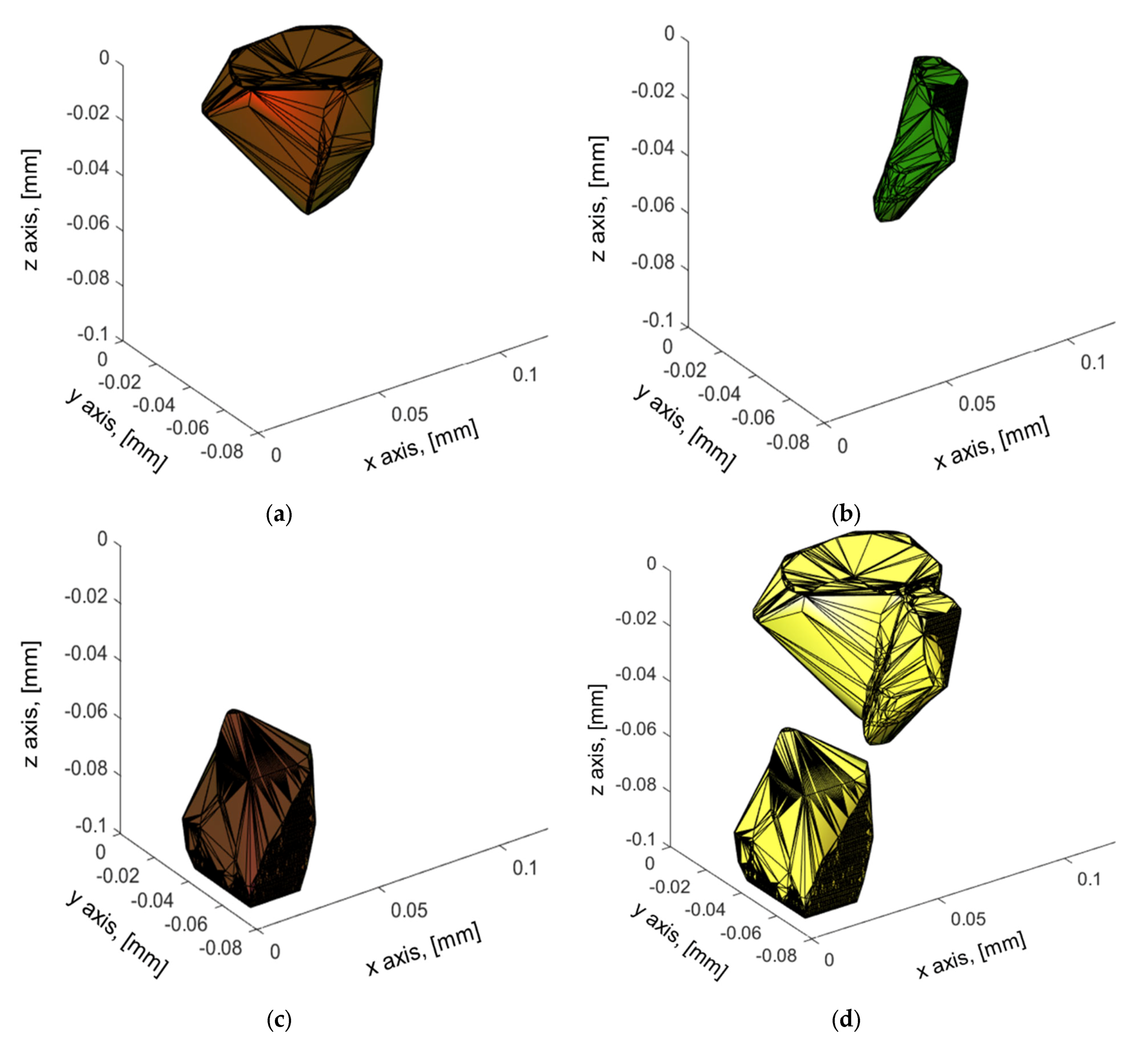
3.3. Nodes and Stacking

When the metallographic microscope used in this paper is set to 500× magnification, the resolution per pixel is approximately 0.063 μm; the micrometer accuracy for measuring the height is 0.01 μm. Consequently, the boundary expressed by the (x,y) coordinates obtained from the MG picture is drawn with a relatively large number of nodes compared to the height z, and higher spatial resolution than necessary. This reduces the computational speed during three-dimensional imaging, as well as forming needle-like surfaces up and down. To overcome this problem, if the number of nodes forming the boundary is reduced, the shape of the layer may be distorted. Accordingly, in this section, we examined how effective it is to reduce the number of nodes forming the boundary of the organization.
Let the pixels of the camera (microscope) be as defined by Equation (12). Generally the ratio of vertical and horizontal pixels is such that m/n = 4/3. The spatial resolution of the image, which can be obtained using the microscope, depends on the optical lens system and can be expressed by Equation (13).
R c = m × n       ( pixels )
R p = w × h       ( μ m )
where w and h   are the width and height of each image. The quantitative distance between each pixel can be derived from Equation (14)
P = w / n       ( μ m / pixels )
Here we were using m = 2048 and obtaining w = 130   ( μ m ) . Therefore, P would be 130 / 2048   ( μ m / pixels ) , corresponding to 0.063   ( μ m / pixels ) . However, as indicated in Table 1, the height of each layer after polishing was 1 2   μ m . If we use P = 0.063   ( μ m / pixels ) , the lateral surface of the crystal will be expressed as shallow needle-like squares, and the surface lacks uniformity, due to the small value of P . In order to reproduce the result well, we defined P as expressed in Equation (15), with P = P × r and r = 30 60 .
P = w / n       ( μ m / pixels )
Figure 6a is a polygonal figure drawn by the boundary coordinates obtained by the above-mentioned algorithm using the picture shown in Figure 4c. There are 3084 polygonal vertices, represented by solid blue lines. Then, the polygons expressed by 1028 vertices skipping three each were expressed by green dot-lines, and the polygons expressed by skipping nine by 343 dots were expressed by circular lines marked in red. A black dot-line is a polygon expressed by 114 dots that are skipped by 27. In the case of a bay with a complex shape located above the structure, it cannot be expressed by the number of vertices being skipped by 27, but the shape of the bay can be expressed by the marked red circular solid line that is expressed by skipping every nine. This means that detailed regions of the structure can be expressed with a spatial resolution of about 0.57 μm. Meanwhile, Figure 6b shows the area of the polygon as a function of the number of vertices of the polygon. The area of the polygon drawn with 114 vertices by skipping 27 is reduced by about 50%; however, when less than 13 are skipped, the area ratio hardly changes. Therefore, in this study, a boundary with a spatial resolution of 0.57 μm was applied by skipping nine each.
Figure 7a–d shows the boundary with a spatial resolution of 0.57 μm of the microscope’s xy section image for the shape of three layers (#1, #2, #3) along the z-axis height, respectively, which is the result of extraction. In the case of #1 and #2, we see an example of a layer that gradually narrows in width as it is polished. If the layer of #1 in Figure 7d becomes smaller, this means that it can be eventually be divided into several layers as in #2. Figure 8a–c is the results of stacking by extracting the coordinates of the layer’s boundaries #1, #3, #5, and #6 by height. #1 indicates a shape in which the cross-sectional area increases gradually and then decreases again. #3 decreases gradually, and at the same time, #5 increases gradually, and #6 appears. Figure 8d is a top view, and #2 and #3 partially overlap to show that a part of the organization has been merged. On the plus side, the upper part of #1 represents a phenomenon in which the layer is separate as the polishing proceeds into a state in which the upper left layer is integrated.

3.4. Post-Processing

The above result is the stacking of the boundary in each layer, and to understand it as a volume, it is necessary to form a surface connecting the coordinate point of the boundary and the position of the adjacent height. In this study, the results shown in Figure 9 and Figure 10 was obtained using “alpha Shape”, a function that creates a boundary area or volume surrounding a set 2D or 3D point in MATLAB. This 3D graphical function may help to understand the layer or MG by imaging the shape of the layer in 3D.
Due to the large grain selected in layer 8, as shown in Figure 9, it is difficult to understand the original shape of the 3D image. Furthermore, we do not know which data is correct in layer 8, that is to say, whether it is connected to the neighboring grain or not. Therefore, we have to compare four figures, namely the original microscopic image, the extracted boundary image, and two types of stacked volumetric images. The reconstructed 3D grains volume is illustrated in Figure 10.

4. Discussion

In this study, a method and its implementation algorithm for the three-dimensional observation of the microstructure of carbon steel (SA106) was proposed while explaining and illustrating its principle.
The visualization of the shape of the 3D grains with simple equipment, namely a polishing machine, a metallurgical microscope, and some algorithms, is a great advantage. Moreover, it is inexpensive and easy to implement due to its simple technique and does not involve extensive hardware and software.
While the mounted object was being polished, a photograph of the layer was taken using a metallurgical microscope. Subsequently, the metallic MG was reconstructed in three dimensions by assembling and processing the collected 2D images through local positioning, MG selection, binarization, resizing, stacking (superimposing), and surfacing, which provides very accurate data. The assembly and processing techniques are based on mathematical formulae as described above; the program derived from these formulae is straightforward. It is easily accessible and provides a quick result, making it a simple resource to operate and can be implemented in general-purpose software, e.g., MATLAB, C, C++, Python.
As shown in the example in Figure 6, the MG image is designed by a large number of nodes and will require a lot of computational power. To overcome this, skipping is necessary. However, there is a limit, which should not be exceeded, to not compromise the accuracy of the final results. Skipping by nine, in this case, leads to both minimal resources simulation time and accurately obtained results. Organizational photos may contain personal opinions. In other words, the shredded pieces may, in fact, be the tip of a large layer. If this personal subjectivity is expressed in three dimensions, a somewhat objective judgment is possible.
Notwithstanding non-destructive testing techniques, three-dimensional imaging grains will be one of the most widely used techniques in the near future. Firstly, for its numerous advantages listed in the introduction. Another interest is to be able to reconstruct the shape of the microstructure, which may allow the evaluation and prediction of the material’s behavior under stress, damage, heat treatment effects, etc., and a variety of research has been carried out in this area [19,44,45].
The reconstructed 3D grains volume, as illustrated in Figure 10, from the processed 2D images is of significant interest and may be useful for our future research in the field of non-destructive evaluation using mainly electromagnetic and ultrasonic testing to better understand structural properties at the microstructural level. In addition, the generation of a three-dimensional grains structure may also broaden the scope of applications, especially in the field of materials science, designing structural materials, and investigation of engineering materials.
In the last few years, thanks to numerical models and the increase in computing and processing capacity, it has become possible to obtain precise models and simulations of complex material properties, especially microstructures, using advanced software and modeling techniques [46,47,48]. The software algorithms developed under MATLAB employed are complementary to the experimental work, and the combination of the two leads to more accurate and realistic grain representations with a very acceptable simulation time. In addition, the method allows the creation of microstructures with the exact shape and size of the grains and offers the possibility of selecting one or more grains, as illustrated in Figure 7, Figure 8 and Figure 10.

5. Conclusions

Three-dimensional imaging of metallic grain by stacking the microscopic images was successfully applied to obtain 3D grain volume from processed 2D images. This method can be applied as a useful tool for the characterization of metal grains. It is ready to be used in industrial steel applications. It has been pointed out that the method presented here allows quick and easy use. Furthermore, it does not require many experimental resources.
An efficient technique to avoid positional errors in image piling has been established. Owing to the size of a wide number of nodes, an alternate method was adopted and presented without jeopardizing the precision of the results.
The research finding confirmed that the 3D imaging technique would be suitable for the mechanical properties and also very interesting and promising for studying the visualization of 3D magnetic domains, which is the next step of this research.
Algorithms and experimental techniques are constantly being refined to further improve and enhance the reliability and efficiency of the desired 3D microstructures.

Author Contributions

Conceptualization, J.L.; methodology, J.L., A.B. and Y.-H.H.; software, A.B., J.L. and D.W.; validation, A.B. and J.L.; formal analysis, A.B., J.L. and Y.-H.H.; investigation, J.L. and A.B.; resources, J.L. and D.W.; data curation, J.L., A.B. and D.W.; writing—original draft preparation, A.B. and J.L.; writing—review and editing, A.B. and J.L.; visualization, D.W. and J.L.; supervision, J.L.; project administration, J.L.; funding acquisition, J.L. This paper was prepared with the contributions of all authors. All authors have read and agreed to the published version of the manuscript.

Funding

This work was supported by the National Research Foundation of Korea (NRF) grant funded by the Korea government (MSIT) (No.NRF-2019R1A2C2006064).

Institutional Review Board Statement

Not applicable.

Informed Consent Statement

Not applicable.

Data Availability Statement

Not applicable.

Conflicts of Interest

The authors declare no conflict of interest.

References

  1. Kumar, S.; Shahi, A. Effect of heat input on the microstructure and mechanical properties of gas tungsten arc welded AISI 304 stainless steel joints. Mater. Des. 2011, 32, 3617–3623. [Google Scholar] [CrossRef]
  2. Jang, D.; Kim, K.; Kim, H.C.; Jeon, J.B.; Nam, D.G.; Sohn, K.Y.; Kim, B.J. Evaluation of Mechanical Property for Welded Austenitic Stainless Steel 304 by Following Post Weld Heat Treatment. Korean J. Met. Mater. 2017, 55, 664–670. [Google Scholar] [CrossRef]
  3. Rabung, M.; Kopp, M.; Gasparics, A.; Vértesy, G.; Szenthe, I.; Uytdenhouwen, I.; Szielasko, K. Micromagnetic Characterization of Operation-Induced Damage in Charpy Specimens of RPV Steels. Appl. Sci. 2021, 11, 2917. [Google Scholar] [CrossRef]
  4. Berkache, A.; Lee, J.; Choe, E. Evaluation of Cracks on the Welding of Austenitic Stainless Steel Using Experimental and Numerical Techniques. Appl. Sci. 2021, 11, 2182. [Google Scholar] [CrossRef]
  5. Cook, R.D. Finite Element Modeling for Stress Analysis, 1st ed.; John Wiley & Sons, Inc.: Hoboken, NJ, USA, 1995. [Google Scholar]
  6. Thomas, D.J. Using Finite Element Analysis to Assess and Prevent the Failure of Safety Critical Structures. J. Fail. Anal. Prev. 2016, 17, 1–3. [Google Scholar] [CrossRef] [Green Version]
  7. Müzel, S.D.; Bonhin, E.P.; Guimarães, N.M.; Guidi, E.S. Application of the Finite Element Method in the Analysis of Composite Materials: A Review. Polymers 2020, 12, 818. [Google Scholar] [CrossRef] [PubMed] [Green Version]
  8. Xing, J.; Du, C.; He, X.; Zhao, Z.; Zhang, C.; Li, Y. Finite Element Study on the Impact Resistance of Laminated and Textile Composites. Polymers 2019, 11, 1798. [Google Scholar] [CrossRef] [Green Version]
  9. Raabe, D.; Sun, B.; Da Silva, A.K.; Gault, B.; Yen, H.-W.; Sedighiani, K.; Sukumar, P.T.; Filho, I.R.S.; Katnagallu, S.; Jägle, E.; et al. Current Challenges and Opportunities in Microstructure-Related Properties of Advanced High-Strength Steels. Met. Mater. Trans. A 2020, 51, 5517–5586. [Google Scholar] [CrossRef]
  10. Wu, Q.; Miao, W.-S.; Zhang, Y.-D.; Gao, H.-J.; Hui, D. Mechanical properties of nanomaterials: A review. Nanotechnol. Rev. 2020, 9, 259–273. [Google Scholar] [CrossRef]
  11. Estrada, N.; Oquendo, W.F. Microstructure as a function of the grain size distribution for packings of frictionless disks: Effects of the size span and the shape of the distribution. Phys. Rev. E 2017, 96, 042907. [Google Scholar] [CrossRef] [PubMed]
  12. Ashcroft, I.A.; Mubashar, A. Numerical Approach: Finite Element Analysis. In Handbook of Adhesion Technology; Springer: Berlin/Heidelberg, Germany, 2011; pp. 629–660. [Google Scholar] [CrossRef]
  13. Paknia, A.; Pramanik, A.; Dixit, A.R.; Chattopadhyaya, S. Effect of Size, Content and Shape of Reinforcements on the Behavior of Metal Matrix Composites (MMCs) Under Tension. J. Mater. Eng. Perform. 2016, 25, 4444–4459. [Google Scholar] [CrossRef] [Green Version]
  14. Takeo, K.; Aoki, Y.; Osada, T.; Nakao, W.; Ozaki, S. Finite Element Analysis of the Size Effect on Ceramic Strength. Materials 2019, 12, 2885. [Google Scholar] [CrossRef] [PubMed] [Green Version]
  15. Gad, S.; Attia, M.; Hassan, M.; El-Shafei, A. Predictive Computational Model for Damage Behavior of Metal-Matrix Composites Emphasizing the Effect of Particle Size and Volume Fraction. Materials 2021, 14, 2143. [Google Scholar] [CrossRef]
  16. Ebuchi, T.; Kitasaka, J.; Nagai, T. Non-Destructive Evaluation of Weld Structure Using Ultrasonic Imaging Technique. Mater. Trans. 2012, 53, 604–609. [Google Scholar] [CrossRef] [Green Version]
  17. Savin, A.; Craus, M.L.; Bruma, A.; Novy, F.; Malo, S.; Chlada, M.; Steigmann, R.; Vizureanu, P.; Harnois, C.; Turchenko, V.; et al. Microstructural Analysis and Mechanical Properties of TiMo20Zr7Ta15Six Alloys as Biomaterials. Materials 2020, 13, 4808. [Google Scholar] [CrossRef]
  18. International Atomic Energy Agency. Non-Destructive Testing: A Guidebook for Industrial Management and Quality Control Personnel; International Atomic Energy Agency (IAEA): Vienna, Austria, 1999; p. 296. [Google Scholar]
  19. Ono, K. A Comprehensive Report on Ultrasonic Attenuation of Engineering Materials, Including Metals, Ceramics, Polymers, Fiber-Reinforced Composites, Wood, and Rocks. Appl. Sci. 2020, 10, 2230. [Google Scholar] [CrossRef] [Green Version]
  20. Masumura, R.; Hazzledine, P.; Pande, C. Yield stress of fine grained materials. Acta Mater. 1998, 46, 4527–4534. [Google Scholar] [CrossRef]
  21. Kosoń-Schab, A.; Szpytko, J. Magnetic Metal Memory in the Assessment of the Technical Condition of Crane Girders for the Needs of Safety. J. Konbin 2019, 49, 49–73. [Google Scholar] [CrossRef] [Green Version]
  22. Kosoń-Schab, A.; Smoczek, J.; Szpytko, J. Magnetic Memory Inspection of an Overhead Crane Girder—Experimental Verification. J. KONES 2019, 26, 69–76. [Google Scholar] [CrossRef] [Green Version]
  23. Murakami, K.; Ishimoto, K.; Senoo, T.; Ishikawa, M. Human Robot Hand Interaction with Plastic Deformation Control. Robotics 2020, 9, 73. [Google Scholar] [CrossRef]
  24. Rogovoy, A.A.; Stolbov, O.V.; Stolbova, O.S. The Microstructural Model of the Ferromagnetic Material Behavior in an External Magnetic Field. Magnetochemistry 2021, 7, 7. [Google Scholar] [CrossRef]
  25. Feinberg, B.; Gould, H. Placed in a steady magnetic field, the flux density inside a permalloy-shielded volume decreases over hours and days. AIP Adv. 2018, 8, 035303. [Google Scholar] [CrossRef]
  26. Cullity, B.D.; Graham, C.D. Introduction to Magnetic Materials, 2nd ed.; John Wiley & Sons: Hoboken, NJ, USA, 2011; p. 568. [Google Scholar]
  27. Nestleroth, J.; Davis, R.J. Application of eddy currents induced by permanent magnets for pipeline inspection. NDT E Int. 2007, 40, 77–84. [Google Scholar] [CrossRef]
  28. Xie, Y.; Li, J.; Tao, Y.; Wang, S.; Yin, W.; Xu, L. Edge Effect Analysis and Edge Defect Detection of Titanium Alloy Based on Eddy Current Testing. Appl. Sci. 2020, 10, 8796. [Google Scholar] [CrossRef]
  29. Grishina, D.A.; Harteveld, C.A.M.; Pacureanu, A.; Devashish, D.; Lagendijk, A.; Cloetens, P.; Vos, W.L. X-ray Imaging of Functional Three-Dimensional Nanostructures on Massive Substrates. ACS Nano 2019, 13, 13932–13939. [Google Scholar] [CrossRef] [PubMed] [Green Version]
  30. Yan, H.; Voorhees, P.W.; Xin, H.L. Nanoscale x-ray and electron tomography. MRS Bull. 2020, 45, 264–271. [Google Scholar] [CrossRef] [Green Version]
  31. Siodlak, D.; Lotter, U.; Kawalla, R.; Schwich, V. Modelling of the Mechanical Properties of Low Alloyed Multiphase Steels with Retained Austenite Taking into Account Strain-Induced Transformation. Steel Res. Int. 2008, 79, 776–783. [Google Scholar] [CrossRef]
  32. Kim, J.; Le, M.; Park, J.; Seo, H.; Jung, G.; Lee, J. Measurement of residual stress using linearly integrated GMR sensor arrays. J. Mech. Sci. Technol. 2018, 32, 623–630. [Google Scholar] [CrossRef]
  33. Suzuki, M.; Kim, K.-J.; Kim, S.; Yoshikawa, H.; Tono, T.; Yamada, K.T.; Taniguchi, T.; Mizuno, H.; Oda, K.; Ishibashi, M.; et al. Three-dimensional visualization of magnetic domain structure with strong uniaxial anisotropy via scanning hard X-ray microtomography. Appl. Phys. Express 2018, 11, 36601. [Google Scholar] [CrossRef] [Green Version]
  34. Kent, A.D.; Yu, J.; Rüdiger, U.; Parkin, S. Domain wall resistivity in epitaxial thin film microstructures. J. Phys. Condens. Matter 2001, 13, R461–R488. [Google Scholar] [CrossRef]
  35. D’Silva, G.J.; Feigenbaum, H.P.; Ciocanel, C. Visualization of Magnetic Domains and Magnetization Vectors in Magnetic Shape Memory Alloys Under Magneto-Mechanical Loading. Shape Mem. Superelasticity 2020, 6, 67–88. [Google Scholar] [CrossRef]
  36. Lebensohn, R.A.; Kanjarla, A.K.; Eisenlohr, P. An elasto-viscoplastic formulation based on fast Fourier transforms for the prediction of micromechanical fields in polycrystalline materials. Int. J. Plast. 2012, 32–33, 59–69. [Google Scholar] [CrossRef]
  37. Knezevic, M.; Drach, B.; Ardeljan, M.; Beyerlein, I.J. Three dimensional predictions of grain scale plasticity and grain boundaries using crystal plasticity finite element models. Comput. Methods Appl. Mech. Eng. 2014, 277, 239–259. [Google Scholar] [CrossRef]
  38. Tasan, C.; Hoefnagels, J.; Diehl, M.; Yan, D.; Roters, F.; Raabe, D. Strain localization and damage in dual phase steels investigated by coupled in-situ deformation experiments and crystal plasticity simulations. Int. J. Plast. 2014, 63, 198–210. [Google Scholar] [CrossRef] [Green Version]
  39. Ardeljan, M.; Knezevic, M.; Nizolek, T.; Beyerlein, I.J.; Mara, N.; Pollock, T.M. A study of microstructure-driven strain localizations in two-phase polycrystalline HCP/BCC composites using a multi-scale model. Int. J. Plast. 2015, 74, 35–57. [Google Scholar] [CrossRef]
  40. Zhang, D.; Prasad, A.; Bermingham, M.J.; Todaro, C.J.; Benoit, M.J.; Patel, M.N.; Qiu, D.; StJohn, D.H.; Qian, M.; Easton, M.A. Grain Refinement of Alloys in Fusion-Based Additive Manufacturing Processes. Met. Mater. Trans. A 2020, 51, 4341–4359. [Google Scholar] [CrossRef]
  41. Todaro, C.J.; Easton, M.A.; Qiu, D.; Zhang, D.; Bermingham, M.J.; Lui, E.W.; Brandt, M.; StJohn, D.H.; Qian, M. Grain structure control during metal 3D printing by high-intensity ultrasound. Nat. Commun. 2020, 11, 1–9. [Google Scholar] [CrossRef] [PubMed]
  42. Qayyum, F.; Guk, S.; Kawalla, R.; Prahl, U. On Attempting to Create a Virtual Laboratory for Application-Oriented Microstructural Optimization of Multi-Phase Materials. Appl. Sci. 2021, 11, 1506. [Google Scholar] [CrossRef]
  43. Darbandi, P.; Bieler, T.R.; Pourboghrat, F.; Lee, T.-K. The Effect of Cooling Rate on Grain Orientation and Misorientation Microstructure of SAC105 Solder Joints Before and After Impact Drop Tests. J. Electron. Mater. 2014, 43, 2521–2529. [Google Scholar] [CrossRef]
  44. Liu, W.; Lianbc, J.; Aravasde, N.; Münstermanna, S. A strategy for synthetic microstructure generation and crystal plasticity parameter calibration of fine-grain-structured dual-phase steel. Int. J. Plast. 2020, 126, 102614. [Google Scholar] [CrossRef]
  45. Rolchigo, M.R.; Mendoza, M.Y.; Samimi, P.; Brice, D.A.; Martin, B.; Collins, P.C.; Lesar, R. Modeling of Ti-W Solidification Microstructures Under Additive Manufacturing Conditions. Met. Mater. Trans. A 2017, 48, 3606–3622. [Google Scholar] [CrossRef] [Green Version]
  46. Mendoza, M.Y.; Samimi, P.; Brice, D.A.; Martin, B.W.; Rolchigo, M.R.; Lesar, R.; Collins, P.C. Microstructures and Grain Refinement of Additive-Manufactured Ti-xW Alloys. Met. Mater. Trans. A 2017, 48, 3594–3605. [Google Scholar] [CrossRef] [Green Version]
  47. Wong, S.L.; Madivala, M.; Prahl, U.; Roters, F.; Raabe, D. A crystal plasticity model for twinning- and transformation-induced plasticity. Acta Mater. 2016, 118, 140–151. [Google Scholar] [CrossRef]
  48. Qayyum, F.; Guk, S.; Prüger, S.; Schmidtchen, M.; Saenko, I.; Kiefer, B.; Kawalla, R.; Prahl, U. Investigating the local deformation and transformation behavior of sintered X3CrMnNi16-7-6 TRIP steel using a calibrated crystal plasticity-based numerical simulation model. Int. J. Mater. Res. 2020, 111, 392–404. [Google Scholar] [CrossRef]
Figure 1. Specimen adjustment to reduce positioning error. (a) Mounted specimen; (b) Jig for key-hole; (c) After grinding Mounted specimen; and (d) Set specimen on the XY-stage using the key and key-hole.
Applsci 11 07787 g001
Figure 2. Microscopic photograph of the polished layers. (a) 3rd layer; (b) 4th layer; and (c) 5th layer.
Applsci 11 07787 g002
Figure 3. Area selection for local positioning. (a) Reference picture nth layer; (b) Target picture (n + 1)th layer.
Applsci 11 07787 g003
Figure 4. Microscopic photographs with local positioning in a certain area. (a) 17th layer, (55,167) ⦣ (1754,1368); (b) 18th layer, (35,170) ⦣ (1734,1369); (c) 17th layer, (701,161) ⦣ (1120,560); and (d) 18th layer, (681,164) ⦣ (1100,583).
Applsci 11 07787 g004
Figure 5. Algorithms for selection, binarization, and boundary extraction. (a) Select a structure and background; (b) Boundary extraction with voids; (c) Boundary extraction without voids; and (d) Boundary extraction algorithm.
Applsci 11 07787 g005
Figure 6. Changes of shape and area due to reducing the number of nodes which consists of the boundary. (a) Shape changes; (b) Area changes.
Applsci 11 07787 g006
Figure 7. Boundaries at several layers. (a) 3rd layer; (b) 7th layer; (c) 10th layer; and (d) 26th layer.
Applsci 11 07787 g007aApplsci 11 07787 g007b
Figure 8. Stacking boundaries at each height. (a) Stacking of #1; (b) Stacking of #3; (c) Stacking of #5; (d) Stacking of #6; and (e) Top-view of stacking boundaries with four grains.
Applsci 11 07787 g008aApplsci 11 07787 g008b
Figure 9. Three-dimensional imaging of microstructure. (a) 3D image of #1 including layer-8; (b) 3D image of #1 except layer-8.
Applsci 11 07787 g009
Figure 10. Three-dimensional volumetric imaging of grains with except discontinuous layers. (a) 3D image of #1; (b) 3D image of #3; (c) 3D image of #6; and (d) 3D image of three grains.
Applsci 11 07787 g010
Table 1. Height of the polished sample at each layer.
LayerHeight of Layer (mm)
1st Point2nd Point3rd Point4th PointAverage
122.4937022.4787022.5043022.5134022.49753
222.4928022.4768022.5021022.5119022.49590
322.4916022.4751022.5000022.5091022.49395
422.4898022.4729022.4985022.5080022.49230
522.4882022.4713022.4974022.5062022.49078
622.4868022.4709022.4966022.5044022.48968
722.4851022.4685022.4945022.5024022.48763
822.4830022.4673022.4924022.5003022.48575
922.4816022.4655022.4912022.4991022.48435
1022.4802022.4641022.4890022.4970022.48258
1122.4791022.4633022.4875022.4954022.48133
1222.4768022.4614022.4858022.4932022.47933
1322.4757022.4604022.4833022.4909022.47758
1422.4740022.4581022.4817022.4888022.47565
1522.4722022.4570022.4799022.4875022.47415
1622.4712022.4555022.4779022.4863022.47273
1722.4692022.4534022.4764022.4851022.47103
1822.4673022.4525022.4756022.4842022.46990
1922.4658622.4508822.4398022.4825822.46828
2022.4644822.4491822.4722822.4404822.46660
2122.4633822.4478822.4703822.4794822.46528
2222.4618822.4457822.4693822.4779822.46375
2322.4608822.4436822.4668822.4771822.46215
2422.4591822.4423822.4652822.4756822.46063
2522.4578822.4402822.4635822.4736822.45885
2622.4558822.4384822.4621822.4718822.45710
2722.4539822.4374822.4603822.4704822.45558
2822.4519822.4354822.4577822.4696822.45373
2922.4503822.4336822.4557822.4685822.45210
3022.4487822.4325822.4540822.4660822.45038
3122.4472822.4306822.4525822.4651822.44893
3222.4460822.4294822.4516822.4633822.44765
3322.4449822.4272822.4500822.4609822.44583
3422.4438822.4251822.4486822.4596822.44435
3522.4427822.4228822.4474822.4586822.44295
3622.4415822.4218822.4463822.4561822.44150
3722.4400822.4203822.4436822.4552822.43985
3822.4438522.4188022.4421022.4537022.43827
3922.4436422.4156022.4409022.4523022.43630
4022.4347022.4144022.4388022.4509022.43470
4122.4323022.4123022.437622.4495022.43292
4222.4312022.4107022.4362022.4472022.43132
4322.4300022.4096022.4355022.4458022.43022
4422.4292022.4087022.4335022.4446022.42900
4522.4283022.4078022.4315022.4427022.42757
4622.4265022.4062022.4299022.4403022.42572
4722.4257022.4053022.4290022.4387022.42467
4822.4239022.4038022.4277022.4374022.42320
4922.4221022.4017022.4267022.4356022.42152
5022.4207022.4007022.4250022.4343022.42017
5122.4191022.3998022.4235022.4334022.41895
5222.4186022.3984022.4218022.4321022.41772
5322.4170022.3970022.4200022.4303022.41607
5422.4158022.3951022.4186022.4288022.41457
5522.4142022.3930022.4167022.4268022.41267
5622.4130022.3916022.4152022.4255022.41132
5722.4123022.3908022.4134022.4234022.40997
5822.4107022.3888022.4117022.4215022.40817
5922.4086022.3868022.4105022.4200022.40650
6022.4066022.3859022.4089022.4185022.40497
Publisher’s Note: MDPI stays neutral with regard to jurisdictional claims in published maps and institutional affiliations.

