Wind Characteristics in Mountainous Valleys Obtained through Field Measurement

Featured Application

Authors are encouraged to provide a concise description of the specific application or a potential application of the work. This section is not mandatory.

Abstract

The wind characteristics of the mountainous environment in Western China are extremely complex. Many advances have occurred in the study of wind characteristics in plains or hilly areas. However, some limitations remain in the study of mountain passes and riverbanks. We selected a mountain pass and river beach in a certain area as the research objects, then set up observation instruments at different locations to establish temporary observation stations to collect more than one year of measured data. By processing the measurement data during the observation period, the mean wind characteristics and fluctuating wind characteristics of the area were obtained. Through comparison with the standard, we found strong nonstationary characteristics of the wind, such as large deviations between the wind field characteristics values in the standard and measured values, proving the need for wind field observations of mountain passes and riverbanks.

1. Introduction

Wind engineering is a discipline that studies the impact of wind on human engineering and social activities [1]. The research on wind-induced vibrations of bridges is becoming more important with the continuous emergence of bridges with continually record-breaking span lengths. Wind load is now the main control load for the design of long-span bridges. The complex topography of mountainous areas significantly changes the vertical distribution of wind speed and the turbulence structure of the near-surface flowing wind, producing an extremely complicated effect of wind on the structure of the bridge. To study the aerodynamic performance of a bridge structure under wind load and ensure the safety of the bridge, the wind field characteristics at the bridge site must be accurately determined.

Due to the peculiarities of the terrain within which mountain bridges are located, it is difficult to construct a unified quantitative guiding standard for the wind field characteristics of mountain terrain, although some research results have been obtained. Many studies [2,3,4] focused on wind flow over the low, gently sloping terrain where there is no significant separation [5]. The current research on the characteristics of mountain topography and wind fields is focusing on the acceleration effect of top mountain wind speed and the characteristics of turbulence in leeward mountain areas under the effect of inflow [6]. Others examined the effects of multiple mountain wind fields [7]. At present, there are three main analytical methods used to study wind characteristics: field measurement, numerical simulation, and terrain model wind tunnel tests.

The conditions of the model wind tunnel test are easy to control, and the test data are reliable. Xu et al. used the terrain model wind tunnel test method to study the spatial distribution characteristics of a wind field at a bridge site located within complex valley terrain [8]. Gong et al. conducted wind tunnel tests on two-dimensional mountains and three-dimensional symmetrical mountains [9]. Cao et al. studied the influence of ground and mountain surface roughness on the flow separation characteristics of the leeward surface of a mountain in a wind tunnel [10]. Liu et al. studied the influence of six different configurations of ribs on the surface wind pressure on high-rise buildings using wind tunnel experiments [11]. However, limited by the wind tunnel test conditions, the geographical range expressed by the terrain model and the scale adopted are generally small. Therefore, the accuracy of these test results needs to be further studied.

The use of numerical simulation methods to study wind characteristics is also a hot topic. Maurizi et al. conducted a numerical simulation study on a valley wind environment in Northern Portugal [12]. Burlando et al. analyzed the long-term wind observation data from multiple observation stations of complex terrain in a coastal area and obtained the correlation between the wind speed of each observation station and the target point using numerical simulation methods [13]. He et al. numerically simulated the wind field of urban terrain [14]. Ren et al. used numerical simulation to study the characteristics of the wind field in a location and, based on this, proposed a new spatial wind field prediction model for complex terrain [15]. Jubayer et al. also used numerical simulation to study the characteristics of a wind field in a larger area and conducted a topographic test [16]. Liu et al. conducted large eddy simulations (LESs) to study the effect of windward-face-mounted ribs on the flow fields, wind pressure distribution, and aerodynamic forces of different high-rise building models, and finally proposed an empirical configuration equation for the ribs [17]. Although numerical simulation has been widely studied and applied, the setting of inlet wind speed conditions, the selection of the terrain calculation area, and the transition form of terrain boundary are not standardized, leading to insufficient rationality of the calculation results.

Field measurements are the most effective method to obtain wind field characteristics, especially the power spectrum, turbulence intensity, turbulence integration scale, and gust factor in pulsating wind characteristics. To study the characteristics of wind, from early on, researchers have collected wind observations. The most reliable and representative Davenport spectrum was obtained by statistically analyzing nearly 100 strong wind records at different locations and different heights around the world [18,19].

Thomas et al. compared wind speed data measured by Doppler sodars with those measured by anemometers mounted on towers and checked the validity of the Doppler sodars. Hayashida et al. used Doppler radars and Powell et al. used GPS dropsondes to measure wind characteristics near the eye walls of tropical cyclones at altitudes higher than 2000 m [20,21,22,23,24,25]. Toriumi et al. obtained multiple wind speed measurements on the Great Naruto Bridge and Akashi Strait Bridge in Japan and obtained the maximum wind speed over 10 min for typhoons and the maximum wind speed over 10 min for monsoons. After, they conducted correlation studies based on the measured data and compared the findings with the longitudinal pulsating wind empirical formula proposed by Davenport [26]. Masters and Tieleman measured three hurricanes in the Gulf of Mexico at heights of 5 and 10 m using a two-dimensional propeller anemometer and a three-dimensional ultrasonic anemometer. The wind characteristic parameters, such as mean wind speed and direction, turbulence intensity, and turbulence integral scale when the hurricane passed, were obtained [27]. Aksel Fenerci et al. used the long-term wind speed and acceleration monitoring data from Hardanger Bridge to study the relationship between wind load and response processes [28]. Chaurasiya et al. obtained the wind field characteristics of Tamil Nadu, India using a Doppler sodars (sound detection and ranging) system [29]. Baidar et al. obtained observations of the urban wind island effect [30]. Jing et al. obtained the characteristics of wind based on the data obtained from two wind poles located on a hillside and the bottom of a valley [31]. To reliably obtain statistical wind characteristics, Wang et al. incorporated two anemometers into a structural health monitoring system (SHMS) to extensively collect wind data to monitor the wind environment at the site of the Runyon Suspension Bridge (RSB) [32]. Zhou et al. investigated the wind characteristics of the Donghai Bridge site and discussed the mean and turbulent wind characteristics based on six years of field monitoring data [33]. Zhang et al. installed nine anemometers on the 325 m high Beijing Meteorological Tower to systematically analyze the recorded thunderstorm flows [34]. When constructing a bridge in a deep canyon, Yu et al. installed five sets of anemometers on the bridge catwalk to provide an overall analysis of the wind characteristics of the bridge [35].

In this study, we obtained wind observations on a river beach and at the height of the main beam of the bridge using one set of 3D Doppler sodars and two sets of 2D anemometers. And the Doppler radar system was developed by ART (Atmospheric Research & Technology). The 2D ultrasonic anemometer was manufactured by the British company Gill Instruments Limited. Wind data were obtained over a long period. The terrain of the bridge site is quite special. It is a typical mountain pass with river beach terrain, also known as horn-shaped terrain. There are limitations to the research of this terrain. The aim of this study was to obtain the basic parameters of the wind characteristics at the bridge site through wind observation to understand the characteristics of the wind field in the valleys and provide a reference for the wind resistance design of related bridges in similar areas. In this study, we comprehensively analyzed the characteristics of mountain wind. The remainder of this paper is structured as follows: Section 2 describes the bridge surroundings and the measurement system. Section 3 describes the mean wind characteristics, including wind speed and direction. Section 4 introduces the turbulence intensity, power spectrum, and turbulence integral scale. The final section presents the conclusions of the study.

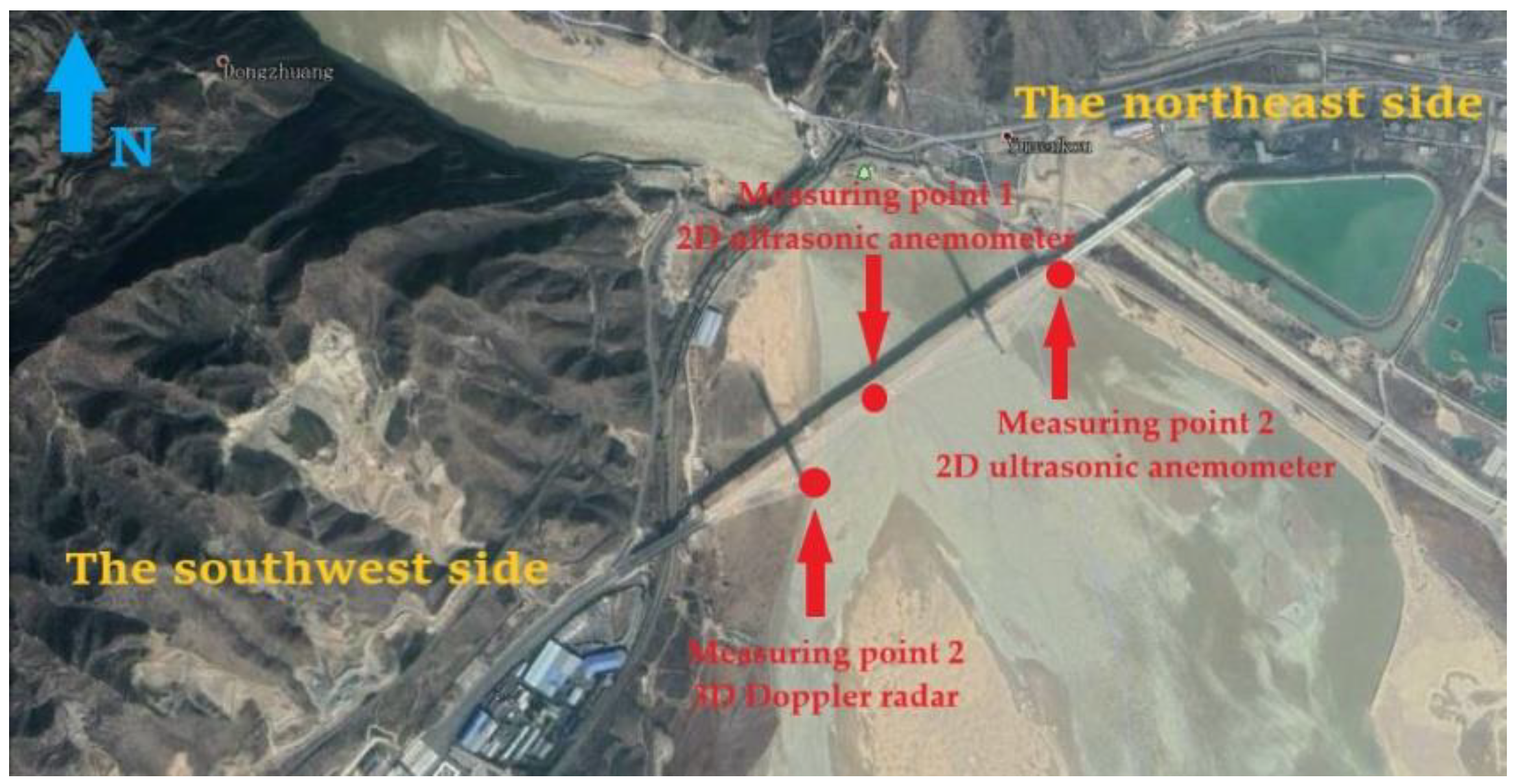
2. Materials and Methods

In this study, we selected the site of a large cable-stayed bridge. Temporary wind observation stations needed to be set up in agreement with the actual needs of the project to ensure that the observations were relevant, representative, and accurate. To understand the spatial distribution characteristics of the wind field around the bridge site, three measuring points were set up at the end of November 2017. One 3D Doppler radar was set on the bank of the river near the main bridge, and its relative position is approximately at the mid-span of the main girder. Two 2D ultrasonic anemometers were set at the height of the main girders, and their relative positions are respectively located at 1/4 of the northeast side and southwest side of the bridge span. The instrumentation details for each site in the observation study are listed in

Table 1. The instrument settings.

Observation Place	Measuring Point Location	Height of Measuring Point or Measuring Range	Instrument Model	Sampling Frequency or Transmitting Frequency
Bridge site	Measuring point 1	33 m	2D ultrasonic anemometer	4 Hz
	Measuring point 2	33 m	2D ultrasonic anemometer	4 Hz
	Measuring point 3	30~200 m	3D Doppler radar	4504 Hz

, and the site location layout details are depicted in Figure 1. The mean wind characteristics were obtained by 3D Doppler radar, and the pulsating wind characteristics were obtained using a 2D ultrasonic anemometer.

3. Results

Mean wind characteristics, such as wind speed and direction, were studied. After the analysis, the pattern of wind speed and direction was obtained, and the influence of the local topography on this mean wind speed and direction was identified.

3.1. Mean Characteristics

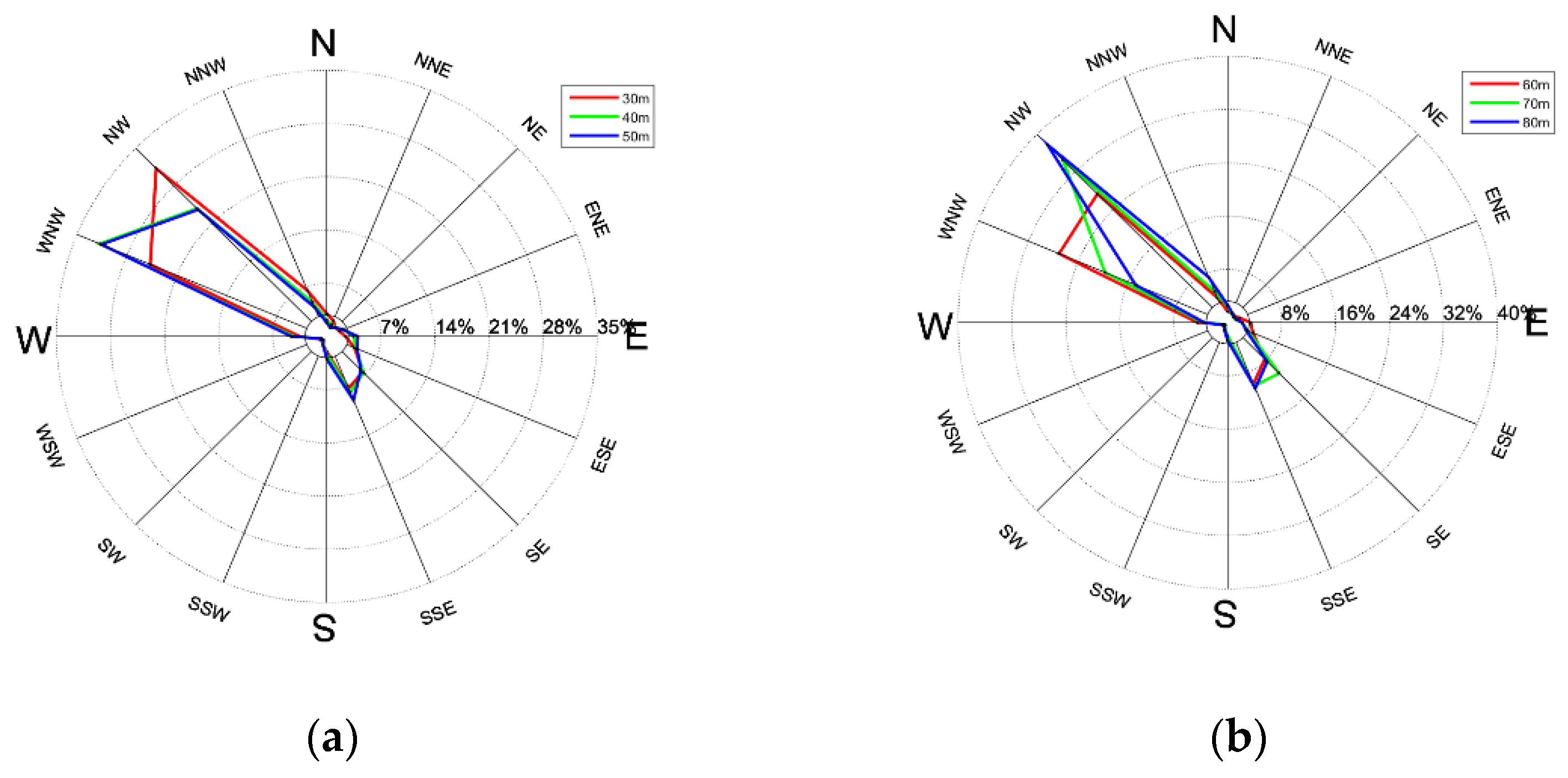
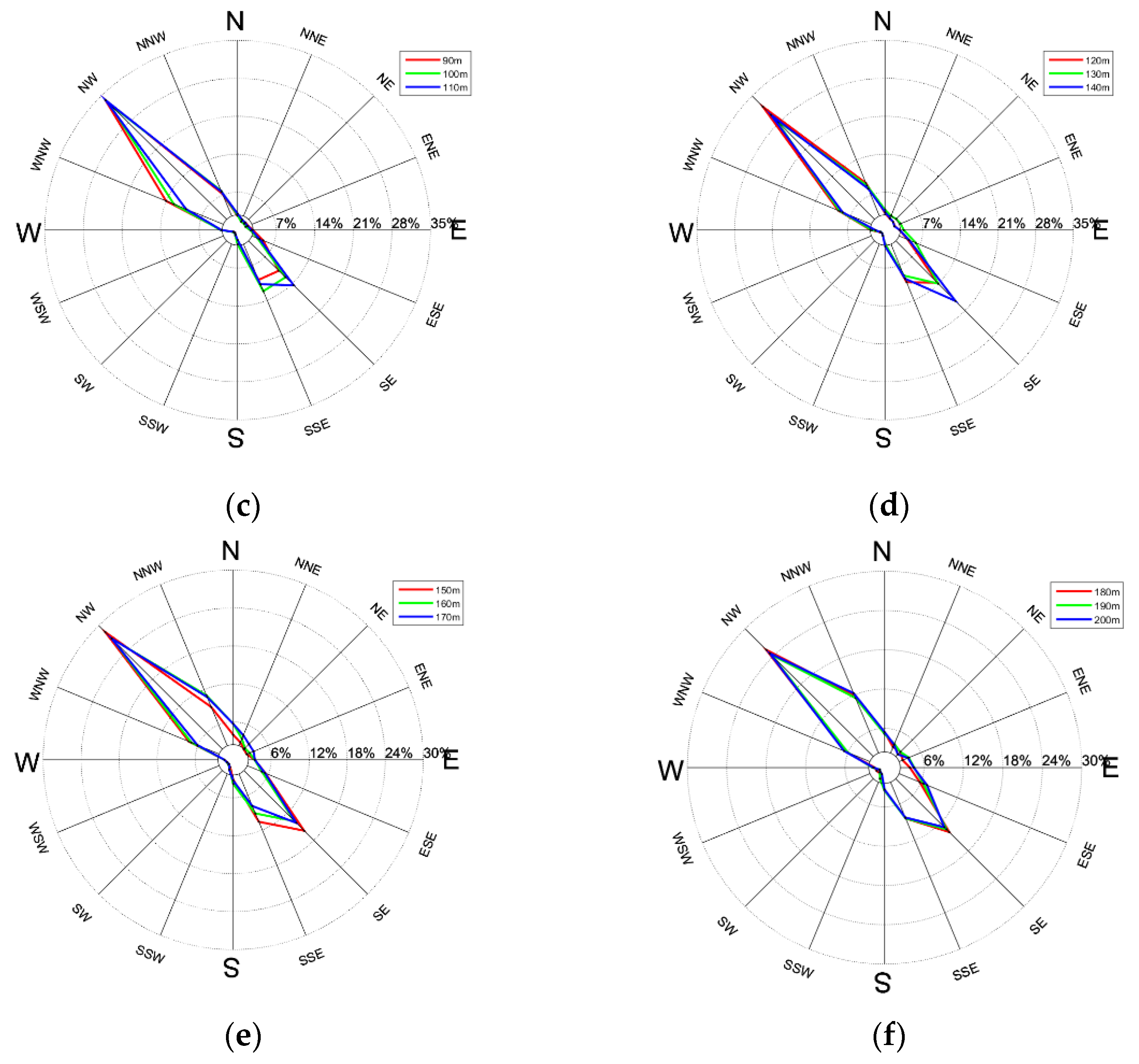
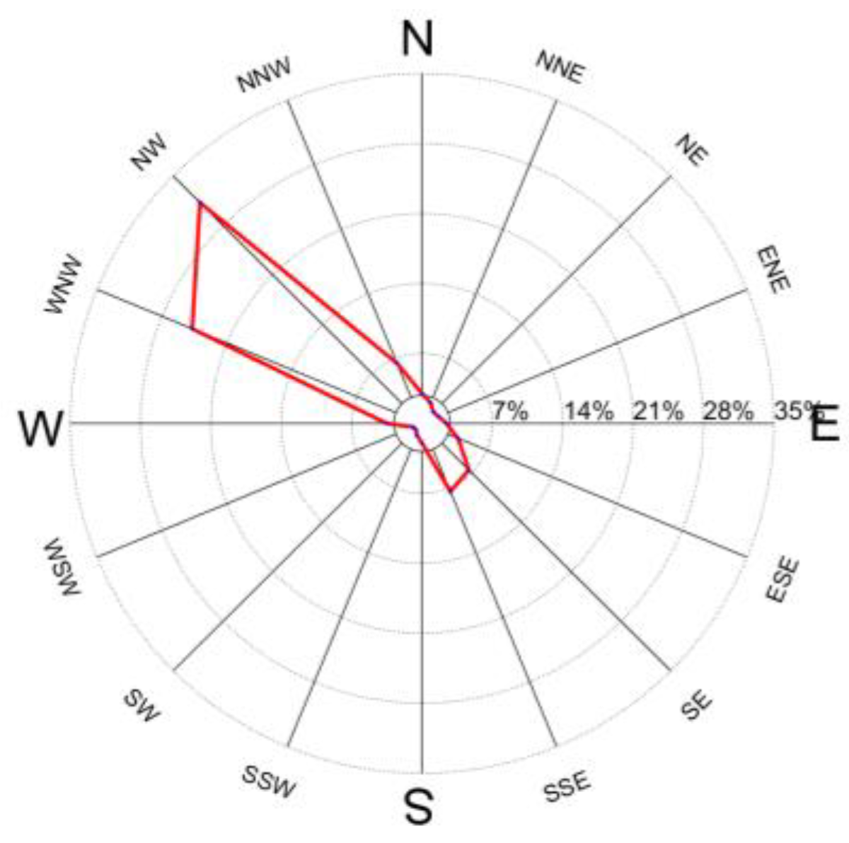
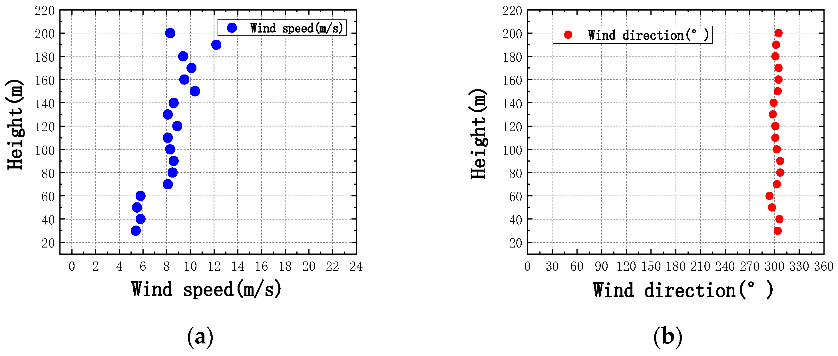
3.1.1. Wind Direction for Mean Wind Speed

The wind rosette is a research tool often used to study wind angles. In this paper, the wind rosette plots were drawn using wind direction samples corresponding to the daily maximum wind speed, as shown in Figure 2. Figure 2 shows the probability magnitudes of the wind direction angles occurring in different directions in the height range of 30–200 m. The distribution frequencies were greatest near the NW at different heights, close to the direction of the centerline of the bell topography (i.e., NW direction in Figure 1). As the height increased, the azimuthal distribution of wind angles increasingly converged toward NW and SE. In the low altitude range of 30–130 m, the frequencies of wind angles between SE and ESE were less than 14%. With the increase in height, the frequency of the wind direction angle in the SE direction increased from 7% to more than 14%, and the corresponding frequency in the NW direction decreased sharply from more than 30%. In addition, as altitude increased, the wind angle distribution increasingly concentrated toward the centerline of the horn-shaped terrain, with an increased proportion of southwesterly wind.

We observed significant differences in the distribution of wind speed and wind direction along the bridge-span direction in this mountainous area. In this study, we examined the differences in wind direction distribution based on the two-dimensional anemometers placed on the southwest and northeast sides and plotted the frequency distribution of wind direction at the two measurement points, as shown in Figure 3.

The sample source for each measuring point plotted is the mean wind direction over 4000 ten-minute windy periods, as shown in Figure 4. The wind rosette at the 30 m altitude, based on the phased-array Doppler radar system, is shown in Figure 4; a large difference between Figure 3 and Figure 4 can be observed. Although the height of the anemometer setup on the southwest side was close to the Doppler radar measurement point at 30 m altitude, there was a difference in the location of the two setups. The Doppler radar was located near the bank of the river on the southwest side, while the anemometer placement was more toward the center of the river. The frequency of the WNW component of the southwest lateral anemometer was significantly higher than that of the Doppler radar results, while the Doppler radar captured the wind direction between the ESE and SSE bearings. The reason for these findings is that the closer the device to the riverbank, the more significant the disturbance produced by the hills and surrounding buildings from the northwesterly wind from the horn, and the more diffuse the wind distribution results. The anemometer was located near the bank of the river. Its main wind direction, WNW, was close to the direction of the continuum between the center of the bell and this measurement point. The incoming front of the anemometer on the northeast side was more open, so its wind direction was widely distributed between the WNW and NW directions. Between these two orientations was the exact opening orientation of the horn. The southwest side was much more obscured by the mountains, and the NW wind blocked the other components of the wind other than the NW bearing. Thus, its main wind direction was closer to the river. We observed a common pattern in the distribution of wind direction on the northeast and southwest sides. The main wind directions all inclined to the center of the river, and the probability of wind direction distribution was smaller near the riverbank position.

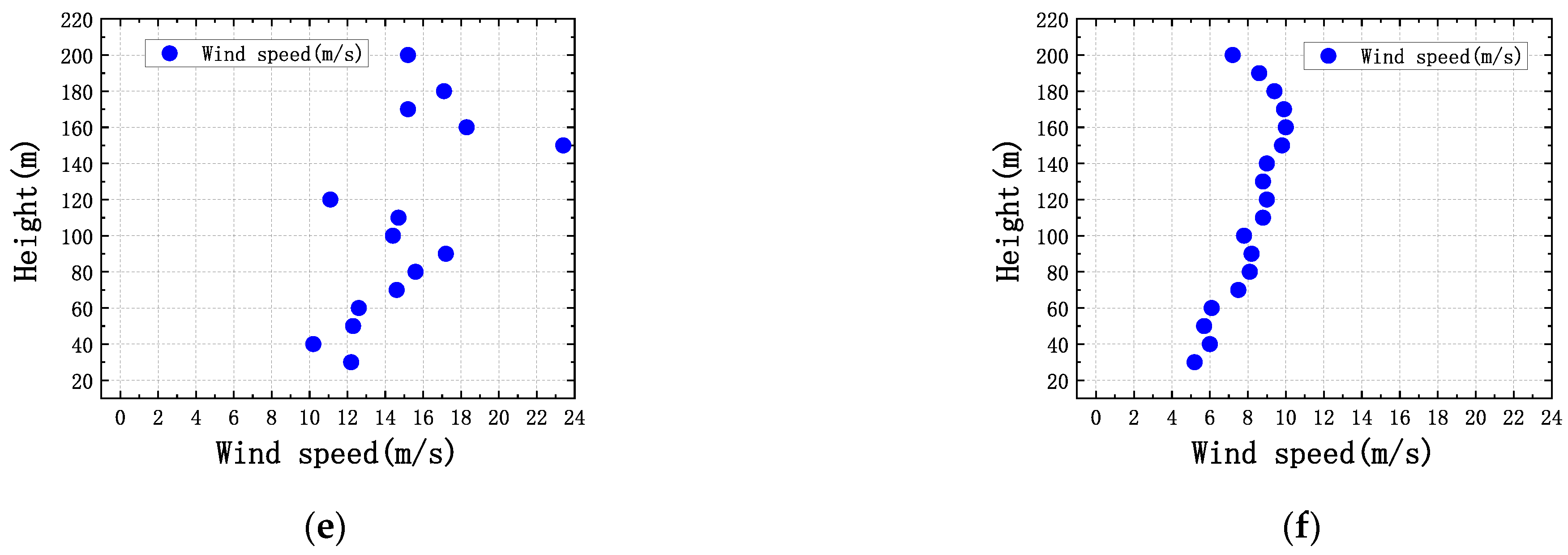
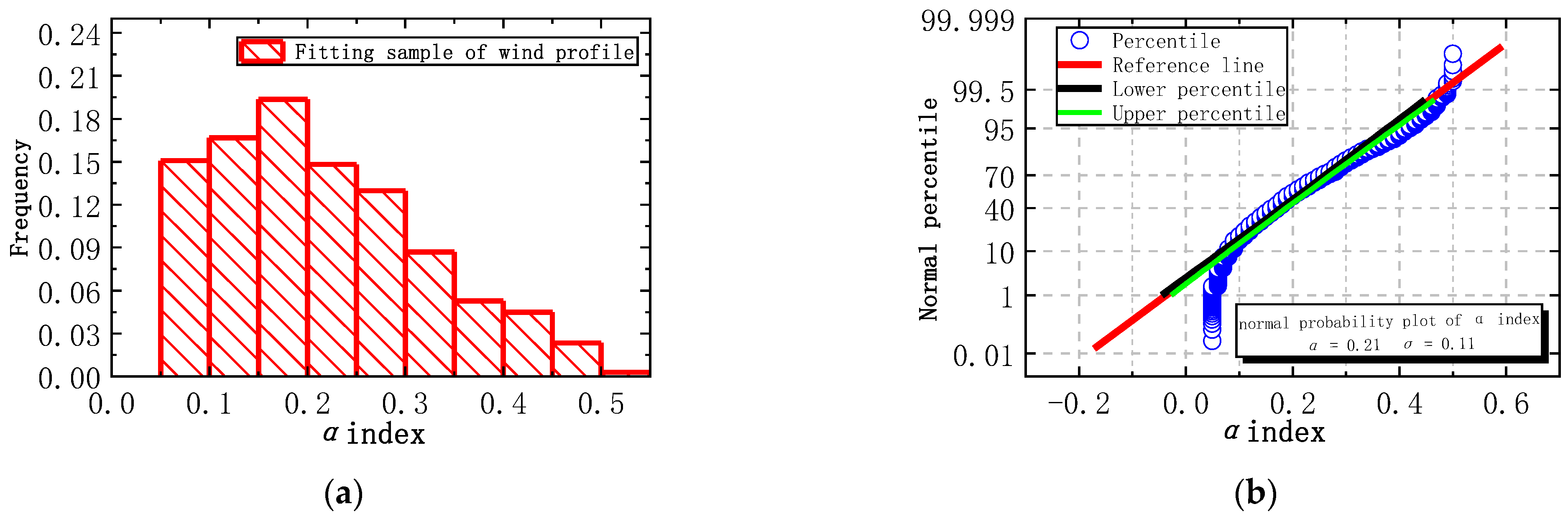
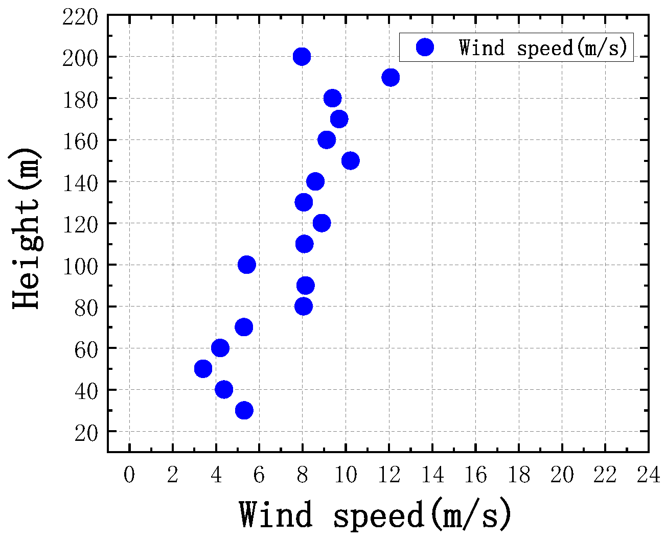
3.1.2. Wind Profile

Within the atmospheric boundary layer, when the topography is homogeneous, the distribution pattern of wind speed along height increases nonlinearly. The curve of the wind speed along the height is called the wind profile. The shape of a site’s wind profile is highly dependent on the roughness of the surface of the site. Based on the theories of logarithmic rate and exponential law, domestic and foreign scholars have obtained the empirical formulae in each country’s norms through statistical analysis of the distribution of the wind field. For windy periods, the formula is generally applicable up to heights of 200 m. Although meteorologists think that the logarithmic law is more accurate, for calculation convenience, the Chinese specification (JTG/T 3360-01-2018) [36] adopts the exponential law form. It is assumed that the distribution of wind speed along the vertical height in the atmospheric boundary layer satisfies the law of exponential change:

$$U(z_2)=U(z_1){(\frac{z_2}{z_1})}^{\alpha }$$

(1)

where z₁ and z₂ represent the heights from the ground, α is a dimensionless parameter determined by the surface conditions, and $U(z_1)$ and $U(z_2)$ represent the wind speed at z₁ and z₂ heights, respectively.

According to the specification, the surface roughness range near the bridge site was assumed to be between 0.22 and 0.30. The 3D Doppler radar can simultaneously obtain wind speed data for 18 altitudes ranging from 30 to 200 m. The actual observation results showed that if all the data from the 18 measurement points are required to be reliable, it will result in a small number of samples that can be processed, and if the unreliable data from the wind speed at each altitude are removed, sometimes too many data are removed, affecting the accuracy of the fit. Therefore, to ensure the accuracy of the study results, the following principle was adopted in this study: after eliminating invalid data from 18 heights in the same time period, the data greater than or equal to 15 were considered to be available for the sample. These were used to fit the wind profile during the observation period. The sample wind speed is also an important factor affecting wind profile fitting results. If the wind speed is too low, the wind profile often does not have a stable form. Therefore, in this study, the mean wind speed at all altitudes greater than 5 m/s was chosen as a threshold, and a total of 4000 study samples were obtained. According to the exponential law using the least squares method to fit the wind profile, the wind profile data were divided into six forms, as shown in Figure 5. The distribution of form (a) is messy, so it is called messy type. Form (b) complies with the exponential law well. The distribution of form (c) is relatively regular. The distribution of form (d) is opposite to the exponential law, so it is called reverse type. The forms of (e) and (f) are like large and small zigzags, respectively. As the height increases, the mean wind speed shows a gradually increasing law in general. Due to the complex topography, the pattern of wind speed variation with height does not fully comply with the exponential law.

Mathematical statistics on the 4000 samples of wind profiles fitted exponentially yielded a sample mean μ of 0.21 and a sample standard deviation σ of 0.11. The frequency distribution histogram is shown in Figure 6. The bridge is located in gentle hilly terrain. According to the Chinese specifications, the surface roughness coefficient for this terrain is 0.22, which is close to the measured value of 0.21. A normal probability plot is used to test whether a set of data obeys a normal distribution. If the sample obeys a normal distribution, the normal probability plot will be a straight line. The shape of the wind profile is the result of many factors, so it was necessary to test whether the α index obeyed a normal distribution. With a confidence level of 95%, the normal probability plot of the α index shows that the normal probability plot is typical of a long-tailed distribution, which means that the statistical distribution of the α index deviates from the mean of the normal distribution.

Figure 7 shows the results of the fitting of the wind profile and the corresponding distribution of the wind angle with height for the same time period. During the same time period, the wind angle remained generally stable at all heights and was distributed around 300° at all heights. This direction is roughly consistent with the direction of the horn pointing downstream of the river in this topography. The analysis of the large number of samples showed that when the wind direction angle was discrete at all heights, the wind speed distribution was also discrete. Additionally, the wind speed and wind direction showed a correlation in terms of distribution stability.

Oblique wind effects are not usually considered in structural analysis, so it was necessary to analyze the wind profile of the cross-bridge with the incoming flow. Figure 8 is the result of fitting the cross-bridge direction wind profile for the same time period as in Figure 7, which breaks down the actual wind speed to the cross-bridge direction for this study. Figure 7 and Figure 8 show a similar pattern of distribution of measured wind speed values, with the cross-bridge to wind profile fit index being slightly smaller than the actual wind speed result.

In areas where the terrain changes dramatically, the wind direction tends to vary considerably throughout the year. Even during the day, the wind direction tends to vary in the morning, midday, and evening. The probability statistics for the α index in Figure 6 reflect the large dispersion of the α index, so the dispersion of the index in the wind profile is likely to be related to wind direction. Figure 7b shows that during 10 min, the wind direction changed little in the range of 30 to 200 m along the vertical direction. The mean value of the wind direction for this time period was taken as a representative value of its wind direction. Figure 9 describes the relationship between the α index and the mean wind direction in polar coordinates using the mean wind direction and the α value as variables, respectively. We found that the distribution of the mean wind direction had a clear tendency to be concentrated between WNW and NNW, which is the same conclusion as that obtained from the wind rose diagram. However, the α values are discrete in all wind angle intervals where the α index appears, so there is no evidence of a relationship between the α index and the mean wind direction. There is a pattern in the orientation with the α values of the wind profiles: few data are distributed between SW and WNW and between NNE and ESE, partly because of the small amount of data in this wind direction and partly because the wind profiles located in these two azimuthal regions are chaotic and do not conform to the exponential law. This means that the incoming currents between these two azimuthal regions are heavily disturbed by the topography and cannot take the form of an exponential law.

The shape of a wind profile tends to change dramatically at different times of the day, particularly in mountainous areas. The Doppler radar system automatically records the 10 min mean wind speed data for the whole day from 00:00 to 24:00. The wind speed waterfall was plotted on a certain day for the four seasons of spring, summer, autumn, and winter, as shown in Figure 10. Figure 10a corresponds to 14 November 2017 in the fall, which had higher wind speeds throughout the day. The wind speeds were lower during the afternoon hours of 14:00 to 16:00, and the shape of the wind profile changed dramatically throughout the day. Figure 10b corresponds to 27 February 2018, with roughly the same time period for the gale speed distribution as in Figure 10a. Figure 10c corresponds to 29 April 2018, in the spring. It can be seen that the wind speed in the early morning hours was the fastest of the day, and the wind speed in the midday to afternoon hours was slower. The shape of the wind profile on this day is reversed, i.e., the wind speed at the bottom was higher than the wind speed at higher altitude. Figure 10d corresponds to 22 July 2018 in the summer and shows that wind speeds between 00:00 and 12:00 were much higher than at other times of the day. In summary, the distribution of strong wind at different times of the day varies widely from season to season. In autumn and winter, strong wind is mainly distributed in the early morning and afternoon. In spring and summer, the strong wind occurs mainly in the early morning. The wind speed at other times of the day is lower. This region is strongly influenced by the monsoons throughout the year, and wind speed varies significantly from one day to the next. Figure 11 shows the monthly maximum wind speed in a year at the temporary station. Figure 11 shows that the maximum monthly wind speed fluctuates sharply with the seasons, and the wind speed in winter and spring is significantly faster than that in autumn and summer.

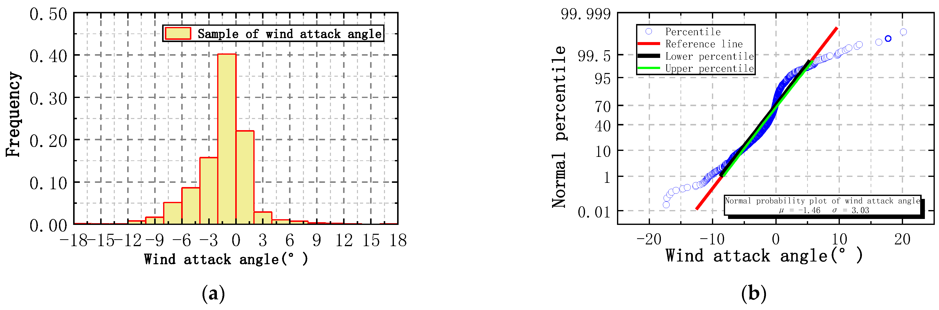
3.1.3. Wind Attack Angle at Mean Wind Speed

The wind attack angle of the mean wind speed is the angle between the main direction of the incoming wind flow and horizontal. The following formula was used for the calculation:

$$\alpha =\arcsin (\frac{u_z}{\sqrt{u_x^2+u_y^2}})$$

(2)

where u_x is the wind speed in the x-direction, u_y is the wind speed in the y-direction, u_z is the wind speed in the z-direction, and α ∈ (−90°,90°).

In the study of wind-induced vibration, the wind attack angle significantly affects the aerodynamic stability of a bridge, so it is important to accurately determine the distribution of the wind attack angle. Usually, the recommended value for wind resistance studies of bridges is −3° to +3°, but this range is only applicable to flat and open areas. Therefore, different from the recommendations of the specifications, the wind resistance study of mountain bridges needs to consider the situation of large angles of attack. When conducting wind tunnel tests, it is even necessary to adjust the wind attack angle to 10°, as Figure 12 shows that the wind attack angles corresponding to each height are discrete in the height range of 30–200 m. Meanwhile, the discrete range of wind attack angles gradually decreases with the increase in height above the ground. At low altitudes below 60 m above the ground, the absolute value of the wind attack angle is large and can even reach nearly 20°. The reason for this finding is that the low altitude is strongly influenced by the terrain, and the wind speed is low, so the air turbulence causes a discrete distribution of the attack angle. As the wind speed increases with height, the valley becomes relatively open and the influence of the terrain gradually decreases; thus, the extreme wind attack angle values decrease, and the distribution interval shortens.

From Figure 12, the mathematical expectation of the wind attack angle tends to move in a negative direction with increasing height. This phenomenon is particularly evident at altitudes between 120 and 200 m. In summary, negative attack angles at the observation point occurred more frequently than positive attack angle attacks, which is caused by the observation point being located downstream of the main incoming wind direction of the horn terrain, i.e., on the leeward side.

The frequency distribution of the wind attack angle at a 30 m altitude is shown in Figure 13. The figure shows that the main distribution interval of wind attack angle is −6° to +6°. There are significantly more negative wind attack angle values than positive values, and the range of wind attack angle with the highest frequency is −3° to 0°. The statistical mean of probability for the wind attack angle sample is −1.46° with a standard deviation of 3.03. The frequency distribution of the wind attack angle is not normally distributed.

3.2. Turbulence Characteristics

Wind turbulence characteristics are an important research topic, especially for large-span bridges located in mountainous area. Turbulence can significantly impact the structural safety of the bridge. In this study, we systematically examined the turbulence characteristics, i.e., turbulence intensity, pulsating wind power spectrum, and turbulence integral scale, based on field measurements.

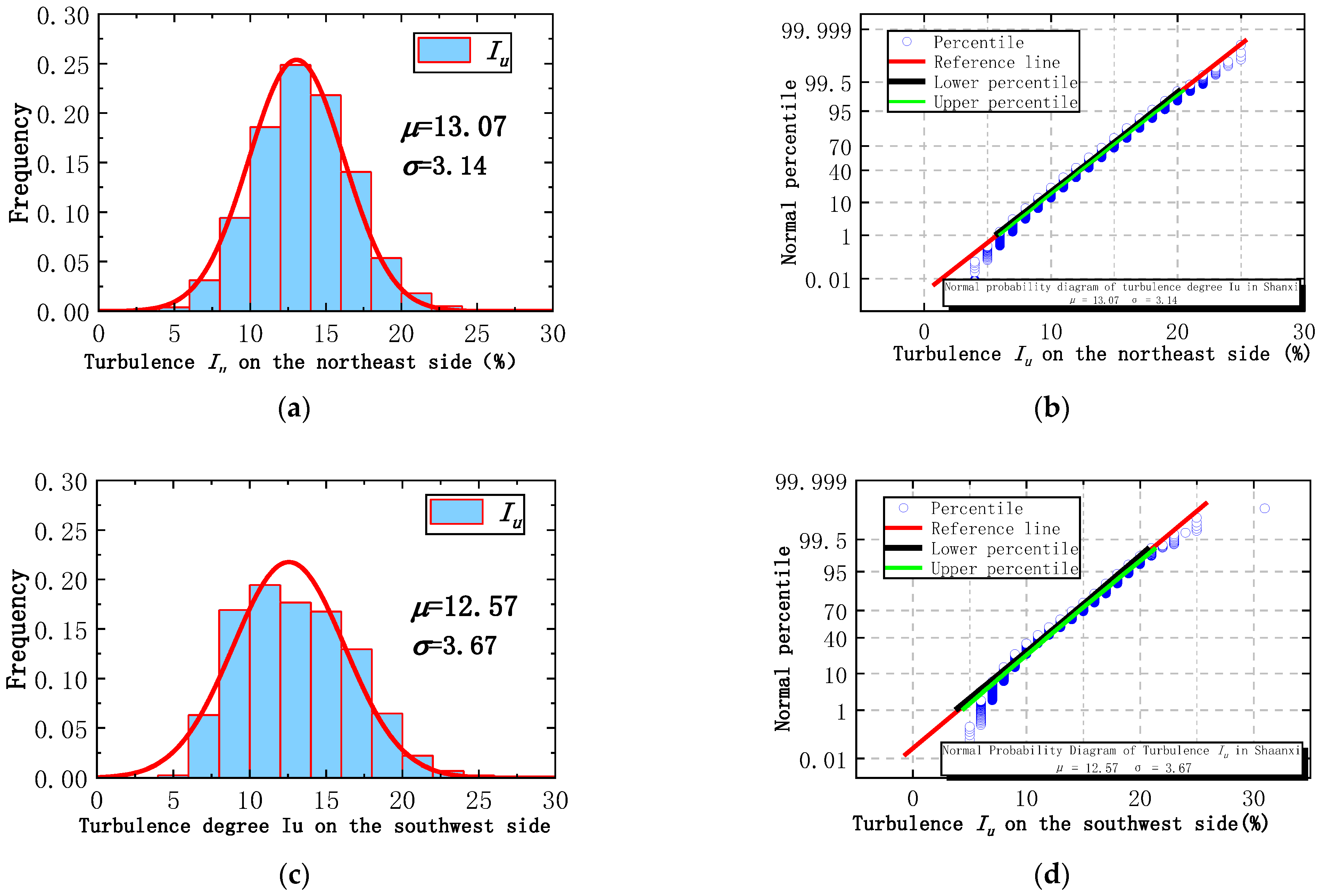
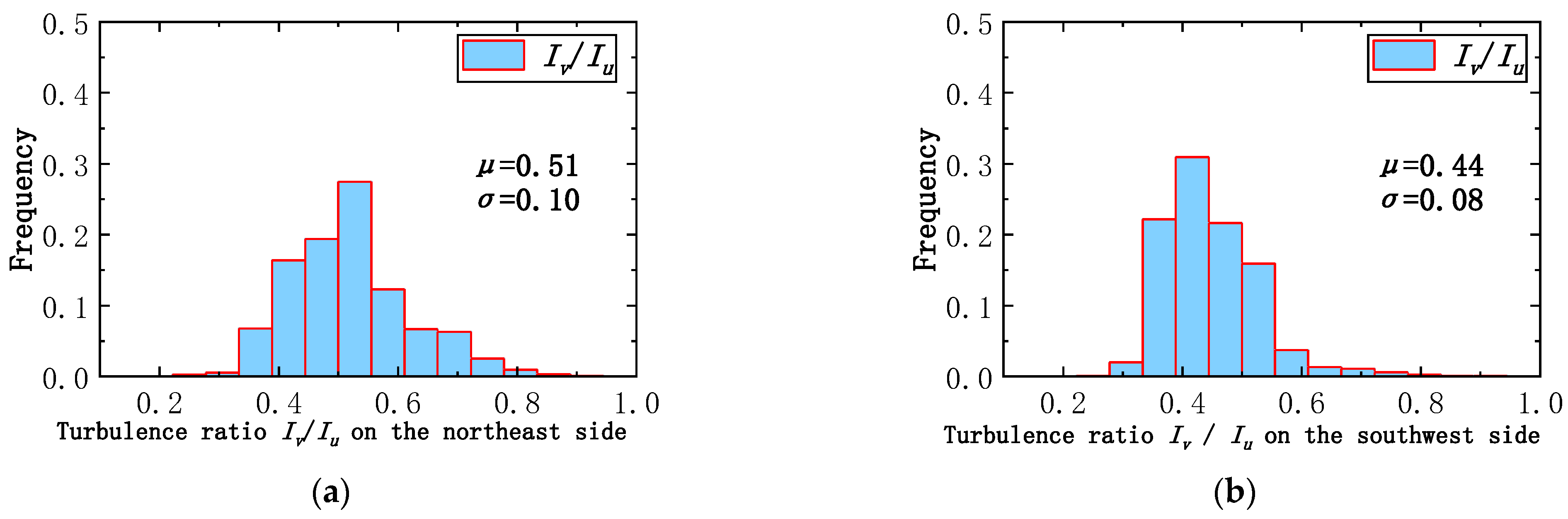
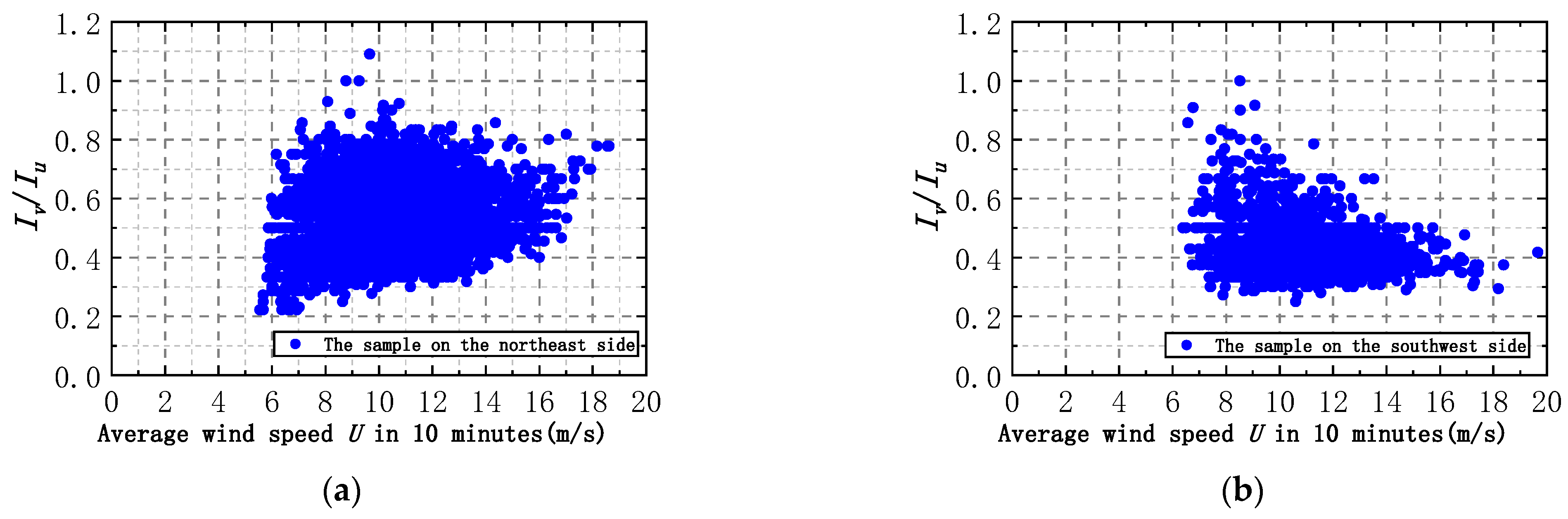
3.2.1. Turbulence Intensity

The turbulence intensity is the ratio of the root mean square to the mean value of the fluctuating wind speed. This is often used to describe the degree of pulsation of natural wind. The turbulence intensity can be computed as

$$I_i=\frac{{\sigma }_i}{\overline{U}}$$

(3)

where I_i is the turbulence intensity in three directions; the subscript i denotes u, v, or w; σ_i is the RMS value of wind speed fluctuations; and $\overline{U}$ is the mean wind speed.

In the Chinese specifications, the relationships of the three turbulence intensities are as follows:

$$I_u:I_v:I_w=1:0.88:0.50$$

(4)

where I_u, I_v, and I_w represent the degree of turbulence in the three directions.

The collected wind speed and direction data were filtered and segmented to obtain nearly 8000 wind samples in 10 min intervals, and the resulting turbulence was calculated by statistical analysis. Figure 14 shows that the mean value of the (10 min mean direction) turbulence I_u in the downwind direction on the northeast side was 13.07% with a standard deviation of 3.14. The maximum value exceeded 22.5%. The mean value of the turbulence I_u in the downwind direction on the southwest side was 12.57%, and the standard deviation was 3.67. The maximum value exceeded 25%.

The mean value obtained by fitting the wind profile according to the exponential law was 0.21. According to the latest version of China’s wind-resistant design specifications for highways and bridges, the recommended value for turbulence intensity in the height range of 30 m < z ≤ 40 m on gentle hilly ground is 21%. The mean values of the turbulence on both the northeast and southwest sides are smaller than the recommended values for this type of surface, and the values are between those recommended for surfaces such as open water and flat open land. This may be related to the excessive wind speed threshold of 5 m/s chosen in this study.

The test of whether the normal distribution is obeyed was performed with a 95% confidence level. From the normal probability plot of the turbulence I_u in the downwind direction on the northeast and southwest sides, we found that the percentile of the sample based on the assumption of normal distribution basically coincides with the normal distribution reference line. The percentile of the two-sided portion lies below the reference line and shows a typical right-handedness distribution. The degree of rightward bias is greater on the southwest side. That is, the frequency of low turbulence in the downwind turbulence I_u sample is higher on the southwest side than on the northeast side.

In Figure 15, the mean value of the crosswind direction (the direction perpendicular to the 10 min mean direction) turbulence I_v on the northeast side is 6.67%, with a standard deviation of 1.99. The maximum value is close to 14%. The mean value of the crosswind direction turbulence I_v on the southwest side is 5.50% with a standard deviation of 1.81. The maximum value is more than 12%. The formula suggested by the design specification for wind resistance of highways and bridges in China is I_v = 0.88I_u. According to the statistical mean value of the measured windward turbulence, the crosswind turbulence I_v on the northeast and southwest sides is 11.5% and 11.06%, respectively. This is much larger than the mean value of the crosswind turbulence obtained from the measurements.

Figure 16 depicts a frequency histogram of the turbulence ratio I_v/I_u for 10 min of mean wind speed U ≥ 5 m/s. The statistical mean value of I_v/I_u on the northeast side is 0.51 with standard deviation 0.10. The maximum value does not exceed 0.9. The statistical mean of I_v/I_u on the southwest side is 0.44 with standard deviation 0.08. The maximum value does not exceed 1.0. The magnitude of I_v/I_u is usually related to the magnitude of the mean wind speed. The higher the wind speed, the smaller the statistical mean of I_v/I_u. Since the wind speed threshold for the gale sample screened in this study was 5 m/s, it is possible that I_v/I_u may be small due to the large values.

In this study, the relationship between the turbulence ratio I_v/I_u and the mean wind speed U was analyzed, and the scatter plots of I_v/I_u and U at the two measurement points on the southwest and northeast sides are shown in Figure 17. We found a significant difference in the distribution form of the scatterplots at the two measurement points on the northeast and southwest sides. The upper limit value of I_v/I_u on the northeast side changed little with increasing wind speed, while the lower limit value of I_v/I_u showed an increasing tendency with increasing wind speed. The upper limit of I_v/I_u decreased significantly with increasing wind speed on the southwest side, while the lower limit of I_v/I_u remained basically unchanged with increasing wind speed. Therefore, the upper and lower limits of I_v/I_u are different at different measurement points, and the relationship between the upper and lower limits of I_v/I_u and the mean wind speed could not be drawn.

Table 2. Distribution interval and expected value of the turbulence ratio corresponding to different wind speed ranges.

Wind Speed Range (m/s)	[4,6]	[6,8]	[8,10]	[10,12]	[12,14]	[14,16]	[16,18]	[18,20]
Iv/Iu interval on the northeast side	0.22~0.60	0.22~0.86	0.25~1.09	0.30~0.92	0.31~0.85	0.38~0.86	0.40~0.82	0.78~0.78
Mean value of Iv/Iu on the northeast side	0.36	0.48	0.5	0.52	0.53	0.55	0.61	0.78
Iv/Iu interval on the southwest side	---	0.27~0.91	0.29~1.00	0.25~0.79	0.30~0.67	0.29~0.50	0.3~0.48	0.29~0.42
Mean value of Iv/Iu on the southwest side	---	0.48	0.46	0.44	0.42	0.41	0.37	0.36

shows the distribution intervals and expected values of the turbulence ratios corresponding to different wind speed ranges. The table shows that the statistical mean of I_v/I_u on the northeast side increased with the wind speed. The statistical mean of I_v/I_u on the southwest side showed a slow decreasing trend with increasing wind speed. The rules of the two measurement points are not uniform. The change rules of turbulence intensity provide a reference for buffeting calculation of long-span bridge under this special terrain.

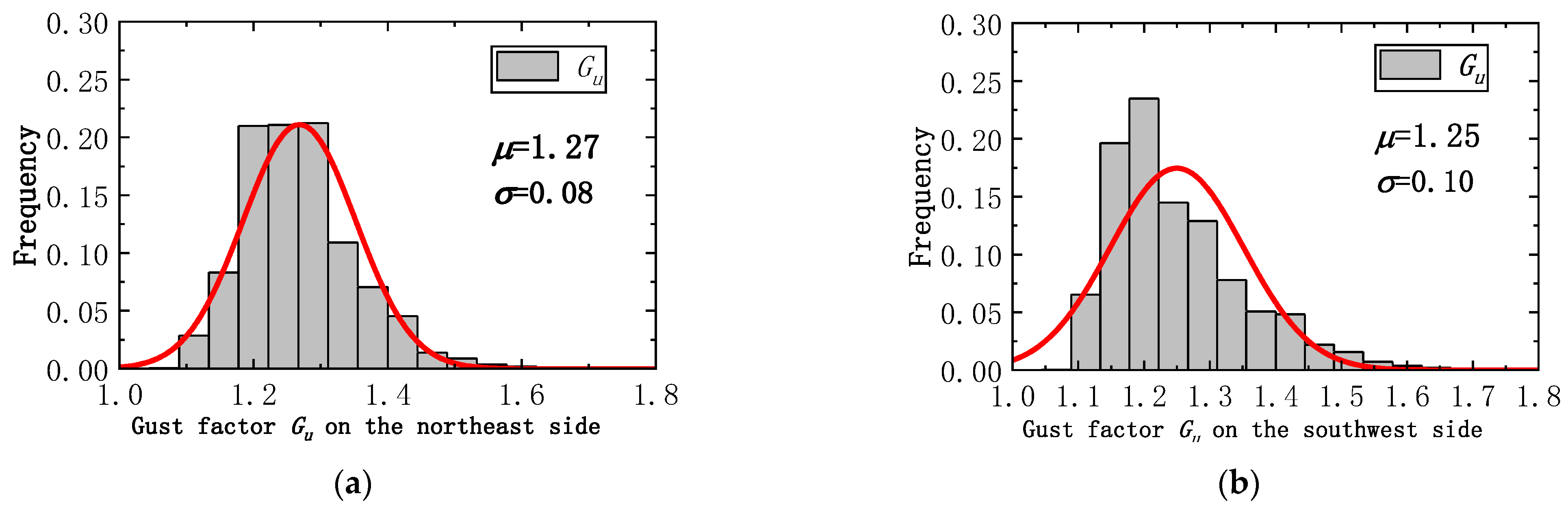
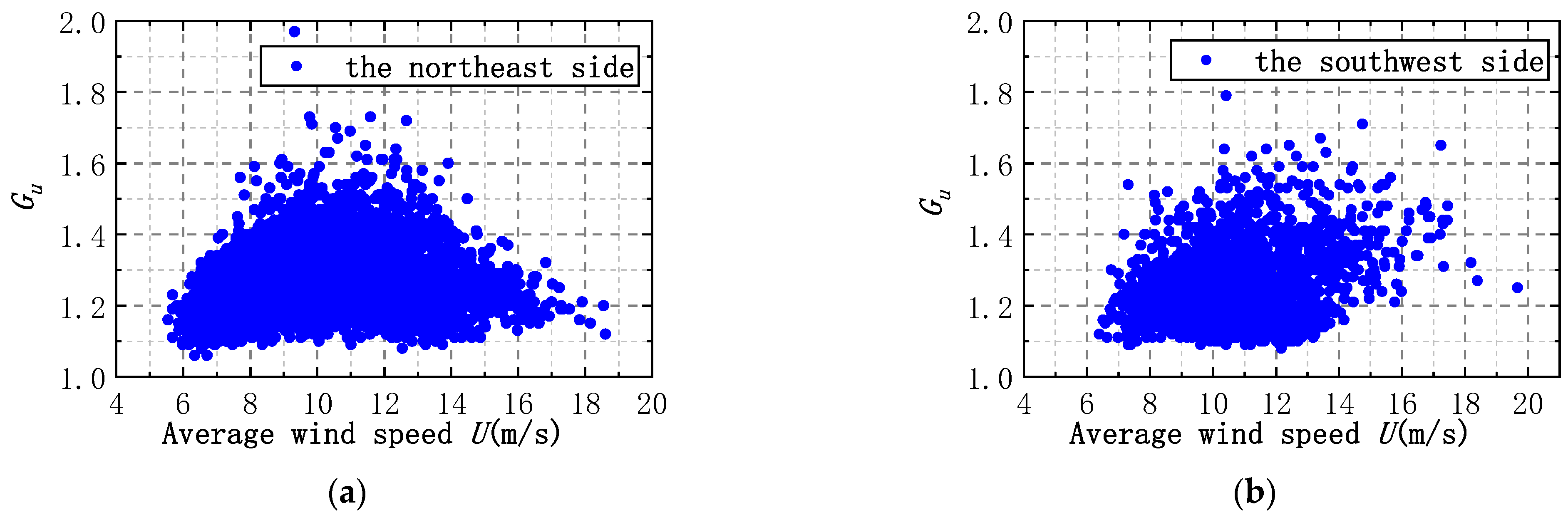
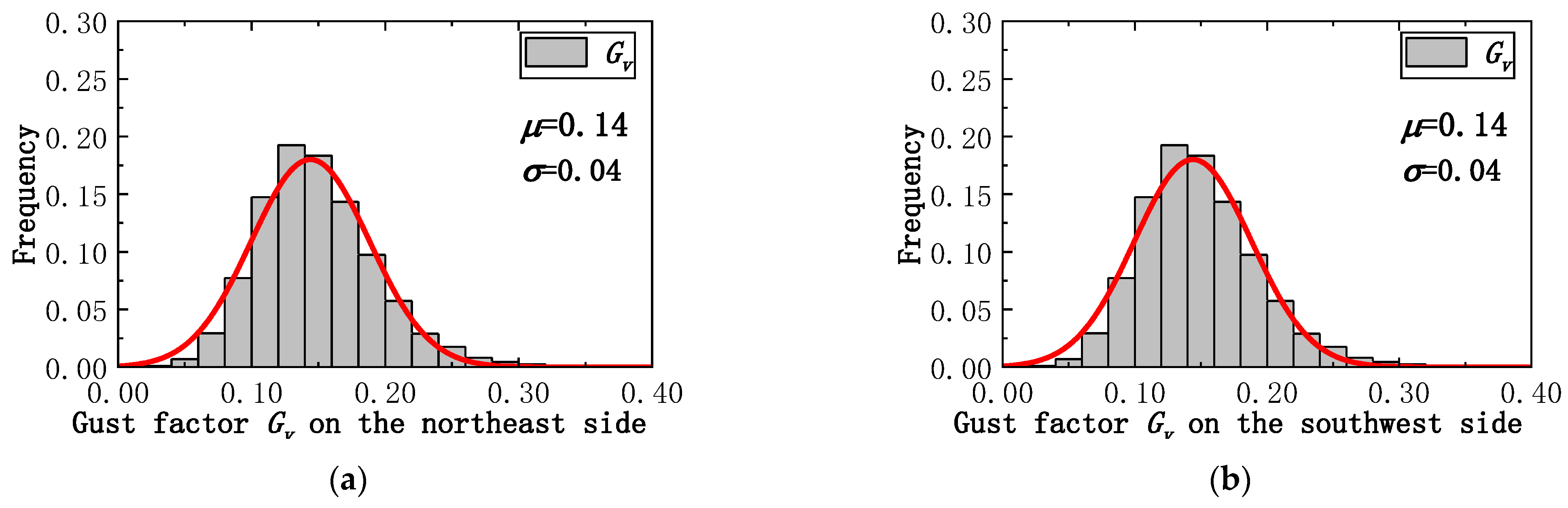
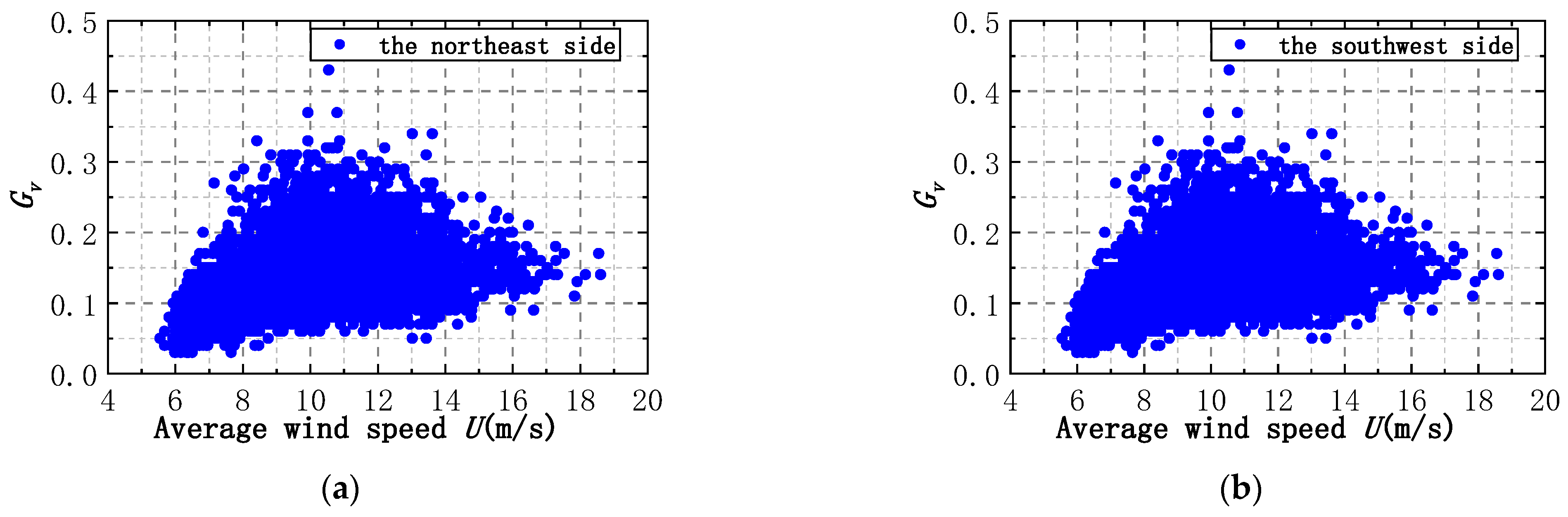
3.2.2. Gust Factor

Gust wind speed is another important factor in the structure’s dynamic response, which is usually expressed as a gust factor. The gust factor is generally defined as the ratio of the maximum 3 s mean wind speed to the 10 min mean wind speed within a 10 min time span. It can be expressed as follows:

$$G_u=\frac{\widehat{U}}{U}$$

(5)

where $\widehat{U}$ is the maximum value of the instantaneous wind speed within a certain time period and $U$ is the mean wind speed of the time period.

The statistical distribution histograms of the statistical probability of the windward gust factor for the two measurement points on the northeast and southwest sides are shown in Figure 18. The mean value of the downwind gust factor G_u on the northeast side is 1.27 with standard deviation of 0.88. The maximum value is 1.60. The mean value of the downwind gust factor G_u on the southwest side is 1.25 with standard deviation 0.10. The maximum value reaches 1.60.

The scatterplots of G_u and U for the two measurement points on the southwest and northeast sides are shown in Figure 19. The scatterplots of the two measurement points on the northeast and southwest sides have similar distribution forms. The main manifestation is the consistent rule of the upper and lower limits of G_u. The upper limit increases with increasing wind speed for mean wind speeds less than 11 m/s and decreases with increasing wind speed for mean wind speeds greater than 11 m/s. The lower limit is always stable around 1.1 as wind speed increases.

The histograms of the probability statistical distribution of the crosswind side gust factors at the two measurement points on the northeast and southwest sides are shown in Figure 20. The mean value of the crosswind gust factor G_v on the northeast side is 0.14 with standard deviation 0.04. The maximum value is above 0.30. The mean value of the gust factor G_v on the southwest side is 0.12 with standard deviation 0.04. The maximum value is also above 0.30.

The scatterplots of G_v and U at the two measurement points on the southwest and northeast side are shown in Figure 21. The distribution rules of the scatterplots at the two measurement points on the northeast and southwest sides are close to each other. The main manifestation is that the upper and lower limits of G_v are consistent. The upper limit increases with increasing wind speed for mean wind speeds less than 11 m/s and decreases with increasing wind speed for mean wind speeds greater than 11 m/s. The lower limit tends to increase slowly with increasing wind speed. The G_u and G_v values at the two measurement points are almost identical for the entire distribution trend.

The statistical distribution histograms of the gust factor ratios G_v/G_u at the two measurement points on the northeast and southwest side are shown in Figure 22. The statistical mean for the northeast side is 0.11 with standard deviation 0.03. The main distribution range is 0.05–0.20. The statistical mean of the southwest side is 0.10 with standard deviation 0.03. The main distribution range is 0.05–0.20. The statistical distributions of G_v/G_u at the two measurement points are quite similar. This result can be used to test the static wind stability of the bridge in this special terrain.

3.2.3. Correlation between Turbulence Intensity and Gust Factor

Some correlation usually exists between the gust factor and turbulence intensity. In this study, the time interval for calculating the gust factor was taken as 3 s. Based on the samples obtained from the measured data, one-dimensional linear regression analysis was performed on the gust factor G_u and turbulence intensity I_u at the two measurement points on the northeast and southwest sides, and the results are shown in Figure 23. The gust factor G_u increases with the increase in the turbulence intensity I_u, and the slope is larger on the southwest side. The regression equation for the northeast side is G_u = 0.98 + 2.19 I_u. The regression equation for the southwest side is G_u = 0.95 + 2.41 I_u.

3.2.4. Wind Power Spectrum

The wind power spectrum is an important tool for measuring the wind turbulence characteristics. In this study, only the downwind pulsating wind power spectral density function was considered to obtain the degree of contribution of different scales of eddies to the turbulent energy in the pulsating wind.

The Kaimal spectrum is currently recommended in the Chinese specifications. The following is an expression for the density function of the downwind power spectrum:

$$\frac{n{S}_u(n)}{u_{*}^2}=\frac{200f}{{(1+50f)}^{5/3}}$$

(6)

where f is a dimensionless parameter; $f=nz/U$ is in the Kaimal spectrum, where $Su$ is the horizontal downwind power spectral density function, z is the height from the ground, n is the frequency of wind, and $u_{*}$ is the friction speed.

Empirical power spectra commonly used in wind engineering also take the form of Harris, Davenport, and Von Karman spectra. For example, the specific expression of the Von Karman spectrum is as follows:

$$\frac{n{S}_u(z,n)}{u_{*}^2}=\frac{2x}{3{(1+70.8x^2)}^{5/6}}$$

(7)

where $L_u\left(z\right)=100{\left(z/30\right)}^{0.5}$ in the Japanese standard and $x=n{L}_u\left(z\right)/{\overline{u}}_z$.

The measured spectra are fitted using a variety of existing empirical spectral formulae, and the results for the northeast and southwest sides are shown in Figure 24 and Figure 25, respectively. The pulsating wind spectrum is usually smaller than the Kaimal spectrum, recommended by the specification in the low-frequency region, and larger than the Kaimal spectrum in the high-frequency region. The cause of this phenomenon is the complex topography of mountainous areas. The topography leads to a large turbulent component of the pulsating wind, and the energy of the turbulence is mainly distributed in the high-frequency region. Therefore, pulsating wind with high turbulence characteristics in mountainous areas with complex topography cannot be accurately and directly described using the readily available empirical function of power spectral density. After comparison, it can be seen that although the measured values deviate from the various spectral curves, the results are closest to the Von Karman spectrum. Since the Von Karman spectrum is now widely used in wind engineering, the Von Karman spectrum was used to fit the power spectrum.

In this study, a two-parameter method was used to fit the power spectrum, and the expression based on the Von Karman spectrum is as follows:

$$\raisebox{1ex}{$n{S}_u(n)$}\!\left/ \!\raisebox{-1ex}{${\sigma }_u^2$}\right.=\raisebox{1ex}{$A{f}_{\mathrm{u}}$}\!\left/ \!\raisebox{-1ex}{${(1+B{f}_u{}^2)}^{5/6}$}\right.$$

(8)

$$f_u{}^2=n{L}_u/U(z)$$

(9)

where n is the frequency; $S_u(n)$ is the measured spectrum value downwind; L_u is the integral scale; σ_u is the standard deviation of the fluctuating wind in the downwind direction, $U(z)=u_{10}{(z/10)}^{\alpha }$; z is the height at a given location; $U(z)$ is the wind speed at height z; $u_{10}$ is the wind speed at 10 m; α is the wind profile index, which is taken as 0.21 based on the actual measurement results; and A and B are the parameters to be fitted.

The frequency distribution histograms of parameters A and B values are shown in Figure 26 and Figure 27. The statistical mean value of parameters A and B on the northeast side are 3.09 and 41.86, respectively. The statistical mean values of parameters A and B on the southwest side are 2.90 and 39.76, respectively. The original values of the Von Karman spectral parameters A and B are 4 and 70.8, respectively, which are quite different from the measured results.

For the fitting results, the standard deviation of fitting is used to measure the error between the measured wind spectrum and various empirical spectra. The expression is as follows:

$$\delta =\sqrt{{\displaystyle \sum _{i=1}^n(\frac{S(i)-S_0(i)}{S_0(i)}}}{)}^2$$

(10)

where $S(i)=\frac{n{S}_u(n)}{{\sigma }_u^2}$ and $S_0(i)=\frac{n{S}_{u_0}(n)}{{\sigma }_u^2}$; $S_u(n)$ is the fitted pulsating wind spectrum or empirical spectrum; $S_{u_0}(n)$ is the measured pulsating wind spectrum; and ${\sigma }_u$ is the standard deviation.

In this study, the above formula was used to calculate the errors of several empirical and fitted spectrum separately from the measured spectrum. The 1250 error samples calculated separately for each spectrum were sorted from smallest to largest and plotted separately on a scatter plot. The sample standard deviations for the northeast and southwest sides are shown in Figure 28 and Figure 29. We found that the sample error of the results obtained using the fitted spectrum was always relatively stable, and the sample standard deviation remained below 1.0.

However, in terms of the minimum sample standard deviation corresponding to several spectra, the fitted spectrum was not advantageous. Particularly for the northeast side, the standard deviation of the fitted spectrum was consistently larger than the other empirical spectra in the region with the smallest sample standard deviation. Other empirical spectra, however, showed a large divergence in standard deviations and a decreasing applicability as the sample size increased.

3.2.5. Turbulence Integral Scale

The turbulence integral scale is a measure of the average eddy size of turbulence. Corresponding to the three directions related to the longitudinal, horizontal, and vertical fluctuating velocity components u, v, and w, respectively, a total of nine turbulent integral scales exist. According to the principle of a smooth random process, the x-direction of the coordinate axis is defined as follows:

$${\mathrm{L}}_a^x=\frac{1}{{\sigma }_a{}^2}{\displaystyle {\int }_0^{\infty }{C}_{a_1{a}_2}(x)}\mathrm{d}x$$

(11)

where a is the direction of the pulsating wind (u, v, or w), $C_{a_1{a}_2}(x)$ is the cross-correlation function of the pulsating component between the two points, and ${\sigma }_a^2$ is the variance of the pulsating wind speed component. The above equation is a theoretical definition. The cross-correlation function of the pulsating components can be rewritten as an autocorrelation function, thus transforming the spatial correlation of two points in the integral scale formula into a temporal correlation of the same point.

The autocorrelation function integral was used to calculate the turbulence integral scale along the downwind pulsating wind speed along the downwind x-axis during the observation period at the bridge site. Figure 30 presents the probability distribution of the integral scale ${\mathrm{L}}_u^x$ based on a large number of wind speed samples during strong wind periods. The figure reveals a wide distribution of integration scales, but mainly concentrated within 100 m. From the statistical results, the value of ${\mathrm{L}}_u^x$ on the northeast side is between 0 m and 650 m. The highest probability is found in the range of 50–100 m, accounting for about 40% of the total, with a mean value of 87.64 m. The ${\mathrm{L}}_u^x$ values on the southwest side ranged from 0 m to 800 m. The 50–100 m range showed the highest probability and accounted for about 40% of these values, with a mean value of 94.13 m.

The histograms of the integral scale frequency statistics for the two measurement points in Figure 30 are similar. To compare the two histograms (H₁ and H₂), it was necessary to define a measure of the concept of similarity, called the degree of similarity,

$$\mathrm{d}(H_1,H_2)=\frac{{\displaystyle \sum _i^n(H_1(i)-\overline{H_1})(H_2(i)-\overline{H_2})}}{\sqrt{{\displaystyle \sum _i^n{(H_1(i)-\overline{H_1})}^2{\displaystyle \sum _i^n{(H_2(i)-\overline{H_2})}^2}}}}$$

(12)

where $\overline{H_k}=\frac{1}{n}{\displaystyle \sum _i^n{H}_k}(i)$, n is the number of statistical intervals in the histogram, and k takes values of 1 and 2.

Equation (12) was used to calculate the similarity coefficients, and the distribution frequencies for each integral scale interval are shown in

Table 3. Frequency distribution of integral scale interval on the northeast and southwest sides.

Integral Scale (m)	Northeast Side Frequency	Southwest Side Frequency	Integral Scale (m)	Northeast Side Frequency	Southwest Side Frequency
[0–50]	36.99	33.26	[400–450]	0.56	0.65
[50–100]	39.29	37.95	[450–500]	0.39	0.48
[100–150]	10.78	14.33	[500–550]	0.17	0.22
[150–200]	4.78	5.78	[550–600]	0.11	0.09
[200–250]	2.96	3.00	[600–650]	0.11	0.13
[250–300]	1.75	2.04	[650–700]	0.07	0.00
[300–350]	1.03	1.04	[700–750]	0.05	0.09
[350–400]	0.92	0.87	[750–800]	0.03	0.04

. The similarity was calculated as 99.53%. The integral scale of the measuring points on the northeast and southwest sides has highly consistent statistical characteristics in the case of large samples. Figure 31 shows the correlation between the integral scale and the mean wind speed. The correlation between the integral scale and the mean wind speed is weak, and the integral scale is highly discrete.

4. Conclusions

In this study, 2D ultrasonic anemometers and 3D Doppler radars were installed on the southwest and northeast sides of a selected site to observe and record the wind environment in the horn-shaped terrain for more than a year. The mean wind characteristics and turbulence wind characteristics, including turbulence intensity, spectral analysis, and turbulence integral scale, were comprehensively analyzed. Statistical analysis of the measured data and local weather station observations revealed that some of wind parameters are almost consistent with the specifications, such as turbulence intensity. Moreover, some of the wind parameters at the observation site differed significantly from the normative recommendations, and the following conclusions were drawn:

(1).

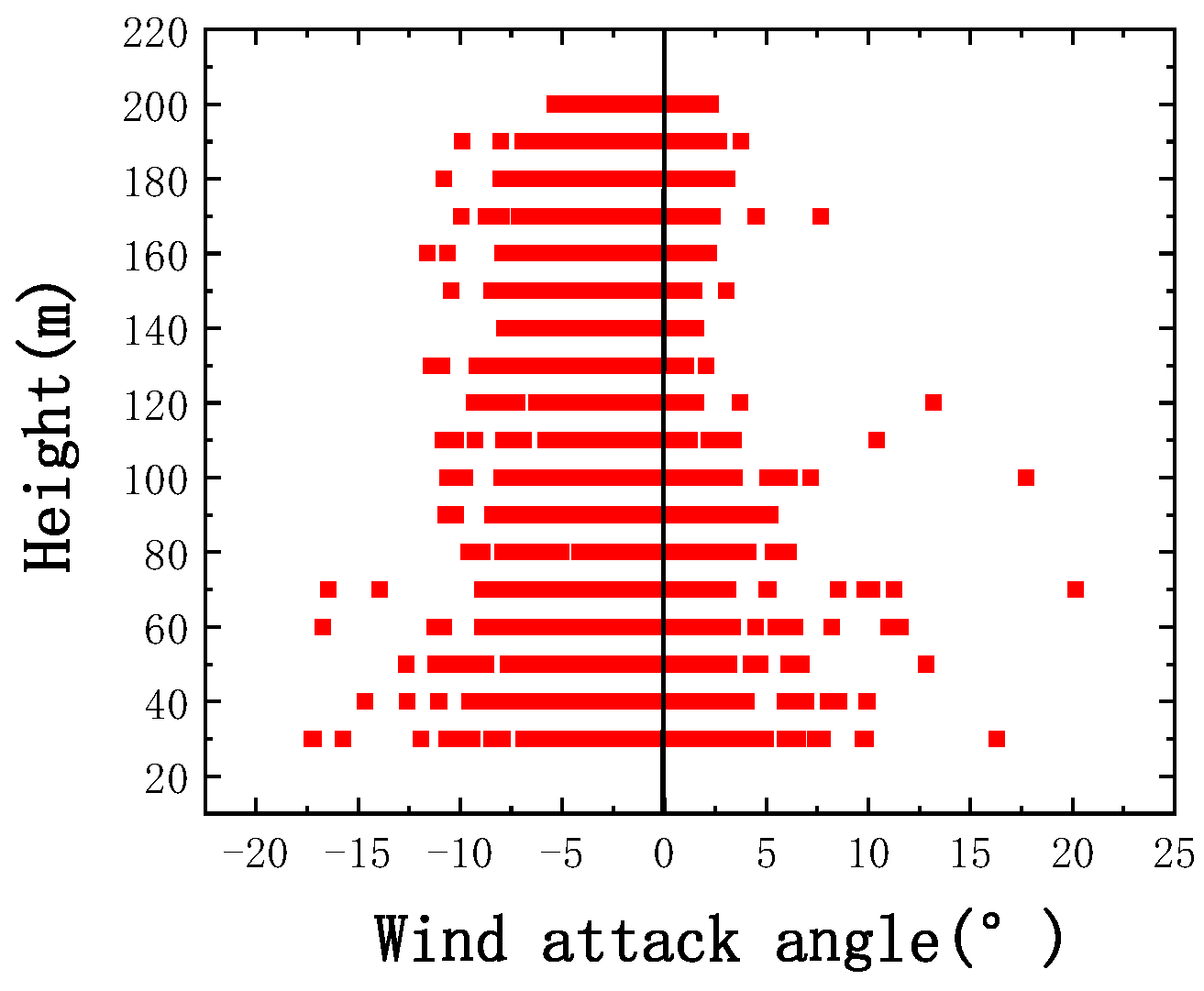
The results indicate that the wind profile index α is about 0.21, and the measuring locations are near the gentle hilly terrain. According to the Chinese specifications, the surface roughness coefficient for this terrain is 0.22, which is close to the measured value of 0.21. However, due to the influence of the complex topography of the area, the wind profile index α cannot fully indicate the surface roughness of the area. As shown in Figure 5, the wind profile data were divided into six forms. This does not match the exponential law. The distribution of wind attack angle in the measured low-altitude range is discrete, even reaching 20°, which is much larger than the ±3° recommended by the specifications. The frequency of negative wind attack angle is greater than that of positive wind attack angle. As height increases, the tendency toward negative tapping angles becomes more obvious. There is a strong correlation between the wind speed profile and the wind direction angle in the observed area. The distribution of wind speed with height in the main wind direction (NW) is well in accordance with the exponential law, while the distribution of wind profile data in other directions is disorganized and irregular.

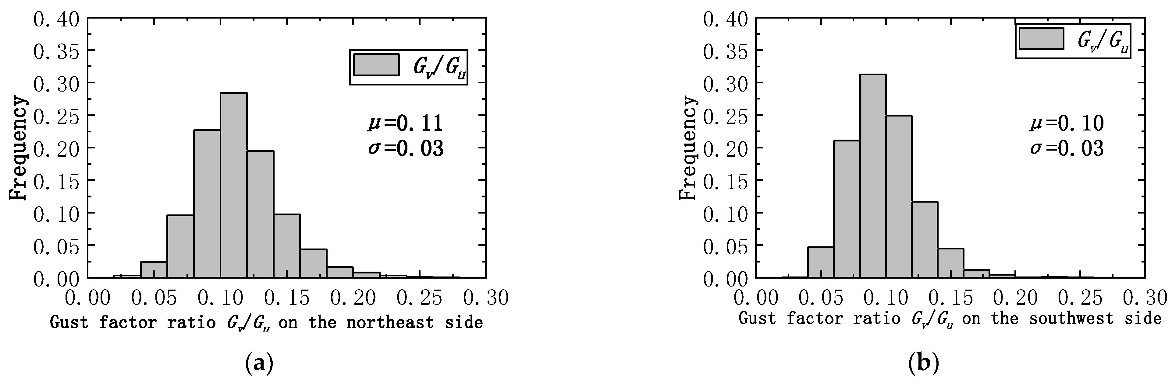
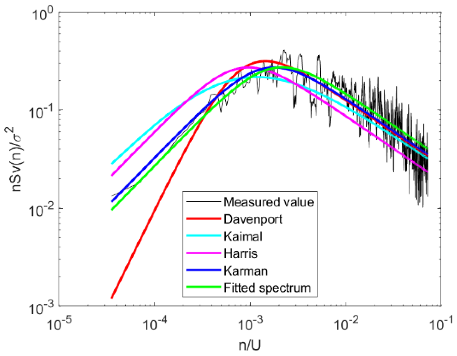
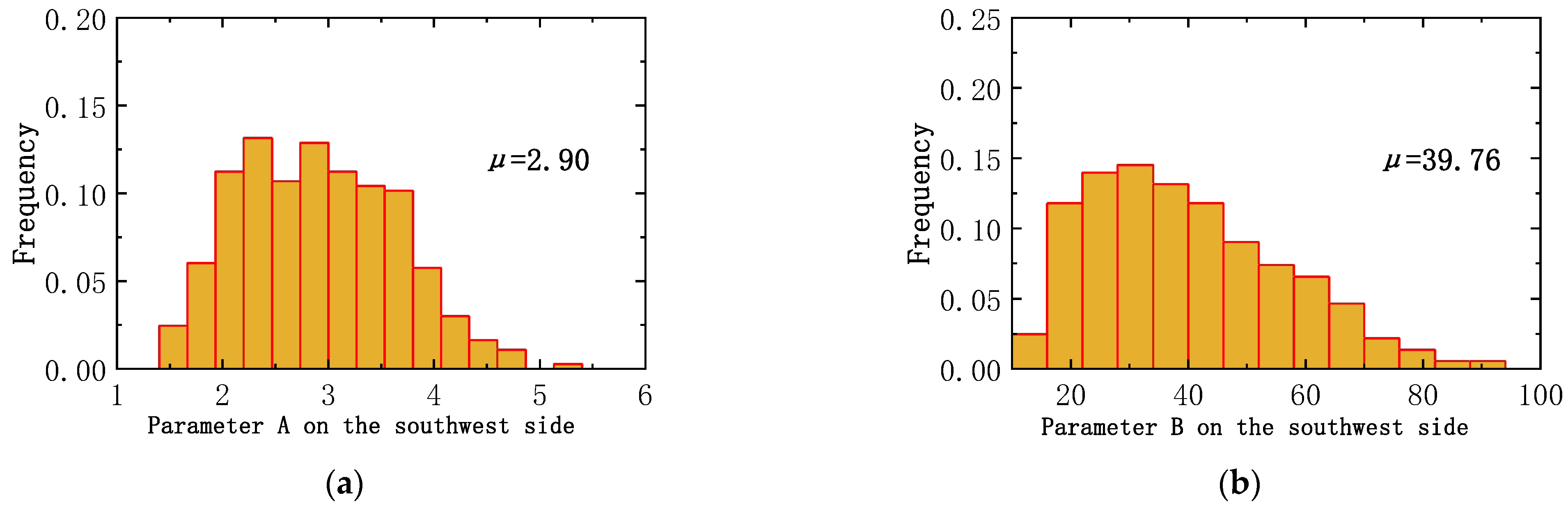
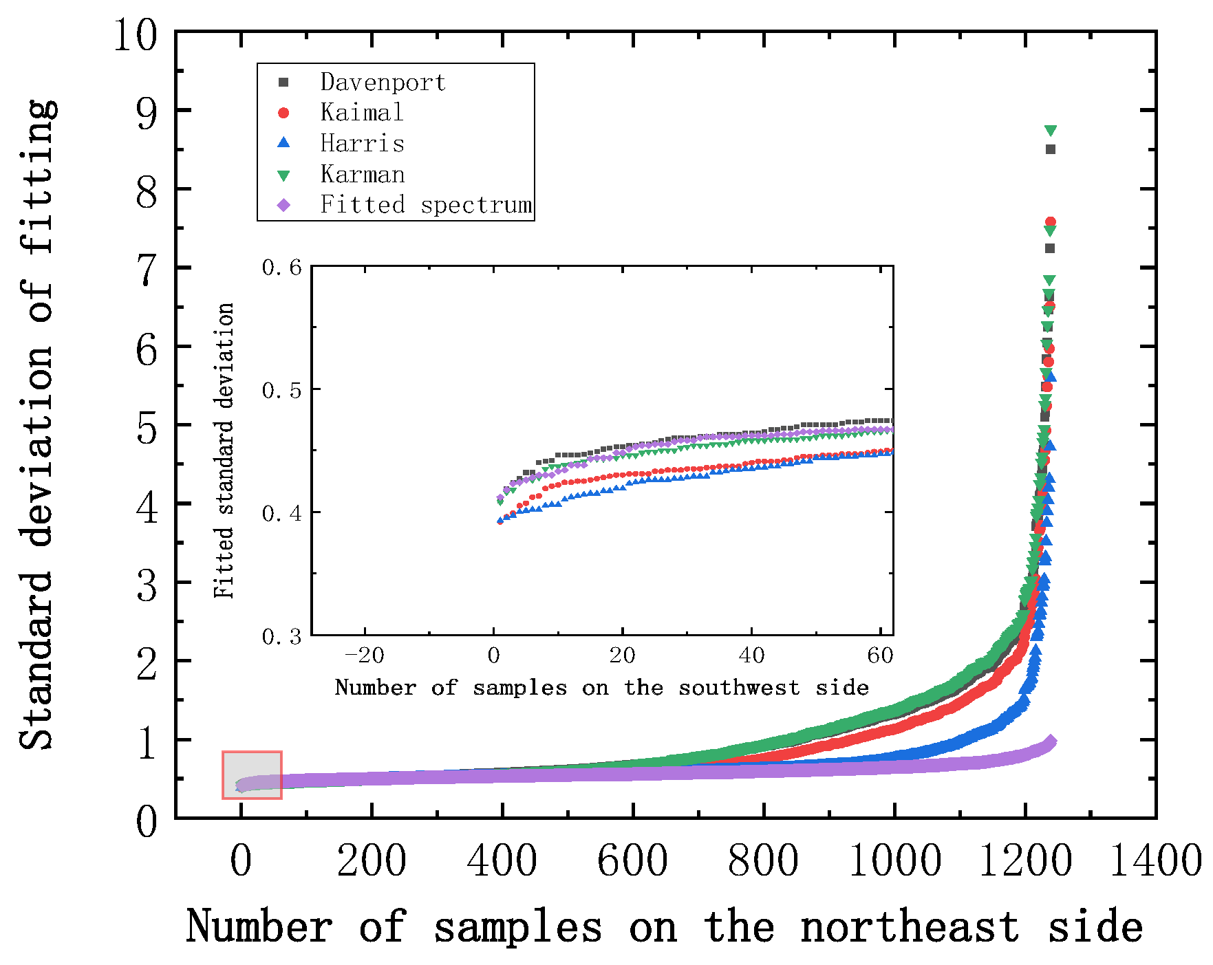
(2).

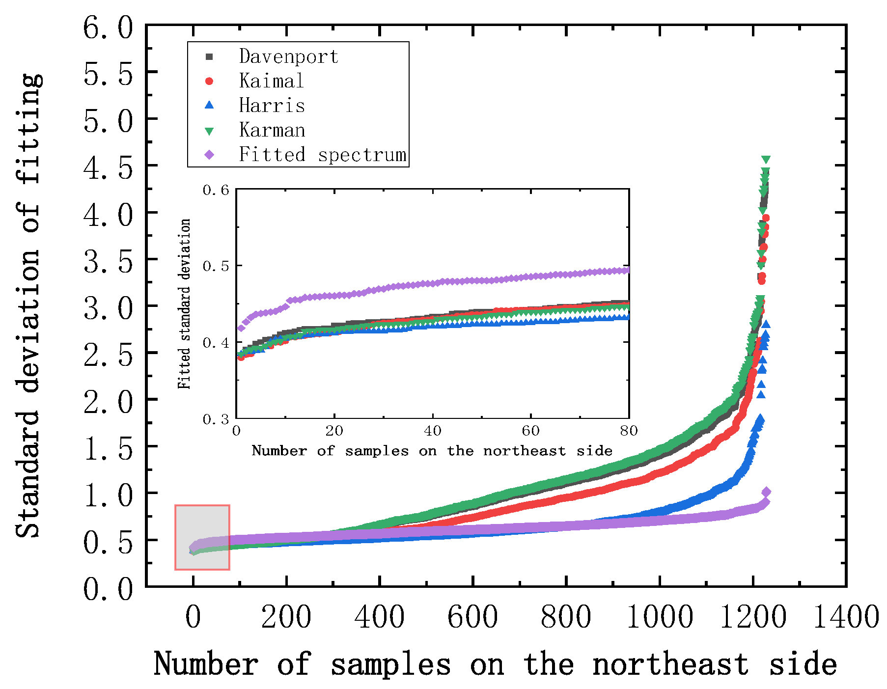
The downwind turbulence intensity degree I_u on both sides of the river channel is about 13%, slightly greater than the 12% recommended value in the norm. However, the ratio of crosswind and downwind turbulence intensity I_v/I_u is 0.46, only 52% of the recommended value of the specification (0.88). This may be due to the topography resulting in the main wind direction (NW and WNW), accounting for a larger component of the incoming wind direction, which in turn results in a reduced degree of crosswind pulsation. We found a strong linear correlation between the gust factor G_u and the turbulence I_u during the observation period, with G_u increasing with the increase in I_u. There is a high turbulent component in the incoming wind velocity in these areas. The high-frequency energy is relatively large, while the low-frequency energy is relatively small. The existing empirical spectra do not provide an accurate description of the measured spectrum. Therefore, the Von Karman spectrum was used to fit the spectrum expressions with good applicability to the wind characteristics.

(3).

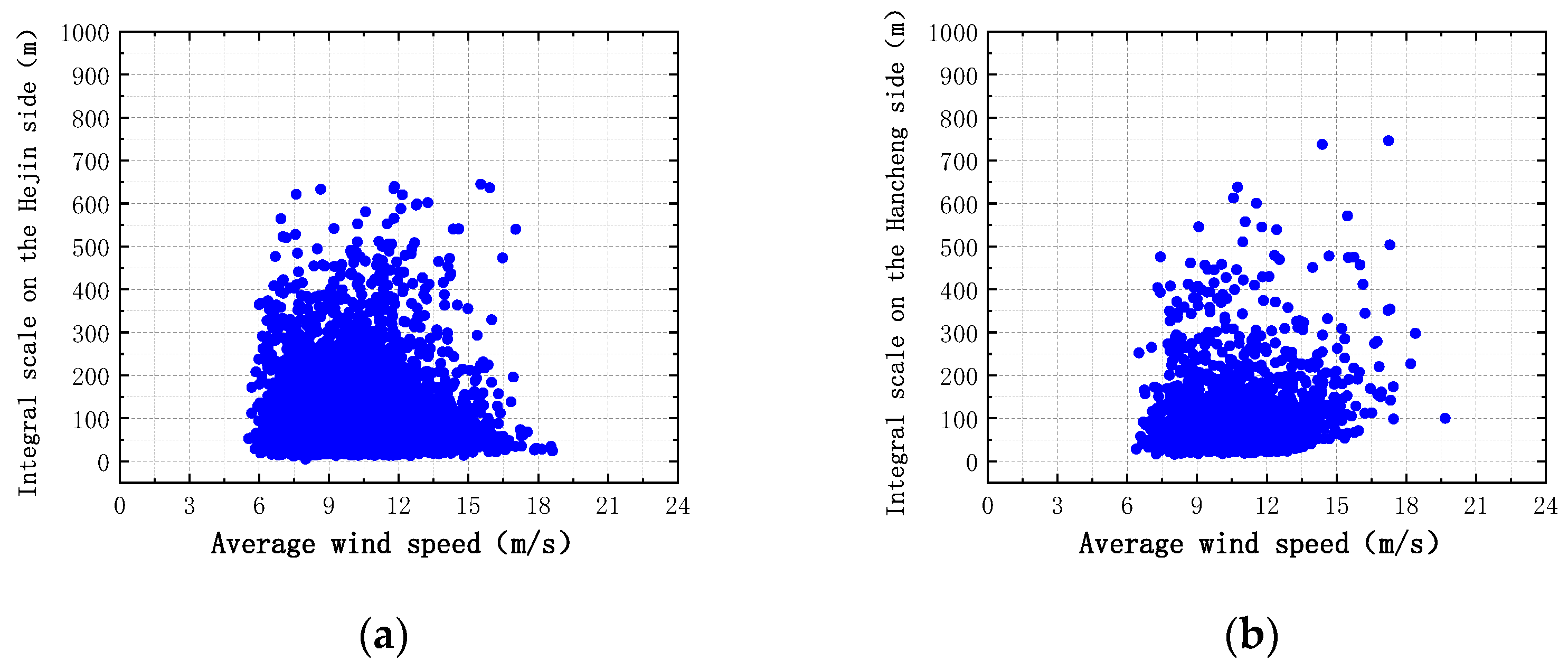
The turbulence integral scale ${\mathrm{L}}_u^x$ on both sides of the river is relatively close, with a statistical mean value of 90 m. Almost half of the sample values had an ${\mathrm{L}}_u^x$ value between 50 and 100 m.

(4).

According to the above analysis results, it can also be seen that the study of the wind characteristics of particular terrain requires special analysis and discussion. The conclusions drawn can then guide the design of the bridges.

References

- Davenport, A.G. Past, present and future of wind engineering. J. Wind Eng. Ind. Aerodyn. 2002, 90, 1371–1380. [Google Scholar] [CrossRef]
- Jackson, P.S.; Hunt, J.C.R. Turbulent wind flow over a low hill. Q. J. R. Meteorol. Soc. 1975, 101, 929–955. [Google Scholar] [CrossRef]
- Teunissen, H.W. Wind-tunnel and full-scale comparisons of mean wind flow over an isolated low hill. J. Wind Eng. Ind. Aerodyn. 1983, 15, 271–286. [Google Scholar] [CrossRef]
- Bowen, A.J. The prediction of mean wind speed above simple 2D hill shapes. J. Wind Eng. Ind. Aerodyn. 1983, 15, 259–270. [Google Scholar] [CrossRef]
- Carpenter, P.; Locke, N. Investigation of wind speeds over multiple two-dimensional hills. J. Wind Eng. Ind. Aerodyn. 1999, 83, 109–120. [Google Scholar] [CrossRef]
- Kossmann, M.; Vögtlin, R.; Corsmeier, U.; Vogel, B.; Fiedler, F.; Binder, H.-J.; Kalthoff, N.; Beyrich, F. Aspects of the convective boundary layer structure over complex terrain. Atmos. Environ. 1998, 32, 1323–1348. [Google Scholar] [CrossRef]
- Raupach, M.R.; Finnigan, J.J. The influence of topography on meteorogical variables and surface-atmosphere interactions. J. Hydrol. 1997, 190, 182–213. [Google Scholar] [CrossRef]
- Xu, H.; He, Y.; Liao, H.; Ma, C.; Xian, R. Experimental study of a wind field in a long-span bridge site located in mountainous valley terrain. J. Highw. Transp. Res. Dev. (Engl. Ed.) 2013, 7, 44–50. [Google Scholar] [CrossRef]
- Gong, W.; Ibbetson, A. A wind tunnel study of turbulent flow over model hills. Bound.-Layer Meteorol. 1989, 49, 113–148. [Google Scholar] [CrossRef]
- Cao, S.; Tamura, T. Experimental study on roughness effects on turbulent boundary layer flow over a two-dimensional steep hill. J. Wind Eng. Ind. Aerodyn. 2006, 94, 1–19. [Google Scholar] [CrossRef]
- Liu, J.; Hui, Y.; Yang, Q.; Tamura, Y. Flow field investigation for aerodynamic effects of surface mounted ribs on square-sectioned high-rise buildings. J. Wind Eng. Ind. Aerodyn. 2021, 211, 104551. [Google Scholar] [CrossRef]
- Maurizi, A.; Palma, J.; Castro, F.A. Numerical simulation of the atmospheric flow in a mountainous region of the North of Portugal. J. Wind Eng. Ind. Aerodyn. 1998, 74, 219–228. [Google Scholar] [CrossRef]
- Burlando, M.; de Gaetano, P.; Pizzo, M.; Repetto, M.P.; Solari, G.; Tizzi, M. Wind climate analysis in complex terrains. J. Wind Eng. Ind. Aerodyn. 2013, 123, 349–362. [Google Scholar] [CrossRef]
- He, J.; Song, C.C.S. Evaluation of pedestrian winds in urban area by numerical approach. J. Wind Eng. Ind. Aerodyn. 1999, 81, 295–309. [Google Scholar] [CrossRef]
- Ren, H.; Laima, S.; Chen, W.-L.; Zhang, B.; Guo, A.; Li, H. Numerical simulation and prediction of spatial wind field under complex terrain. J. Wind Eng. Ind. Aerodyn. 2018, 180, 49–65. [Google Scholar] [CrossRef]
- Jubayer, C.M.; Hangan, H. A hybrid approach for evaluating wind flow over a complex terrain. J. Wind Eng. Ind. Aerodyn. 2018, 175, 65–76. [Google Scholar] [CrossRef]
- Liu, J.; Hui, Y.; Wang, J.; Yang, Q. LES study of windward-face-mounted-ribs’ effects on flow fields and aerodynamic forces on a square cylinder. Build. Environ. 2021, 200, 107950. [Google Scholar] [CrossRef]
- Davenport, A.G. The spectrum of horizontal gustiness near the ground in high winds. Q. J. R. Meteorol. Soc. 1961, 87, 194–211. [Google Scholar] [CrossRef]
- Davenport, A.G. The relationship of reliability to wind loading. J. Wind Eng. Ind. Aerodyn. 1983, 13, 3–27. [Google Scholar] [CrossRef]
- Thomas, P.; Vogt, S. Variances of the vertical and horizontal wind measured by tower instruments and SODAR. Appl. Phys. B Photophys. Laser Chem. 1993, 57, 19–26. [Google Scholar] [CrossRef]
- Vogt, S.; Thomas, P. SODAR—A useful remote sounder to measure wind and turbulence. J. Wind Eng. Ind. Aerodyn. 1995, 54, 163–172. [Google Scholar] [CrossRef]
- Ito, Y.; Naganuma, T.; Kodama, R.; Hanafusa, T.; Sato, J.; Kobayashi, T.; Takeuchi, K.; Suzuki, T. Wind measurements using a Doppler sodar. Wind Eng. JAWE 1996, 1996, 33–38. [Google Scholar] [CrossRef]
- Hayashida, H.; Fukao, S.; Kobayashi, T.; Nirasawa, H.; Mataki, Y.; Ohtake, K.; Kikuchi, M. Remote sensing of wind velocity by boundary layer radar. Wind Eng. JAWE 1996, 1996, 39–42. [Google Scholar] [CrossRef]
- Powell, M.D.; Black, P.G.; Houston, S.H.; Reinhold, T.A. GPS Sonde Insights on Boundary Layer Structure in Hurricanes. In Proceedings of the 23rd Conference on Hurricanes and Tropical Meteorology, Dallas, TX, USA, 10–15 January 1999. [Google Scholar]
- Tamura, Y.; Iwatani, Y.; Hibi, K.; Suda, K.; Nakamura, O.; Maruyama, T.; Ishibashi, R. Profiles of mean wind speeds and vertical turbulence intensities measured at seashore and two inland sites using Doppler sodars. J. Wind Eng. Ind. Aerodyn. 2007, 95, 411–427. [Google Scholar] [CrossRef]
- Toriumi, R.; Katsuchi, H.; Furuya, N. A study on spatial correlation of natural wind. J. Wind Eng. Ind. Aerodyn. 2000, 87, 203–216. [Google Scholar] [CrossRef]
- Masters, F.J.; Tieleman, H.W.; Balderrama, J.A. Surface wind measurements in three Gulf Coast hurricanes of 2005. J. Wind Eng. Ind. Aerodyn. 2010, 98, 533–547. [Google Scholar] [CrossRef]
- Fenerci, A.; Øiseth, O.; Rønnquist, A. Long-term monitoring of wind field characteristics and dynamic response of a long-span suspension bridge in complex terrain. Eng. Struct. 2017, 147, 269–284. [Google Scholar] [CrossRef]
- Chaurasiya, P.K.; Ahmed, S.; Warudkar, V. Wind characteristics observation using Doppler-SODAR for wind energy applications. Resour.-Effic. Technol. 2017, 3, 495–505. [Google Scholar] [CrossRef]
- Baidar, S.; Bonin, T.; Choukulkar, A.; Brewer, A.; Hardesty, M. (Eds.) Observation of the Urban Wind Island Effect; EDP Sciences: Les Ulis, France, 2020. [Google Scholar]
- Jing, H.; Liao, H.; Ma, C.; Tao, Q.; Jiang, J. Field measurement study of wind characteristics at different measuring positions in a mountainous valley. Exp. Therm. Fluid Sci. 2020, 112, 109991. [Google Scholar] [CrossRef]
- Wang, H.; Guo, T.; Tao, T.-Y.; Li, A.-Q. Study on wind characteristics of runyang suspension bridge based on long-term monitored data. Int. J. Struct. Stab. Dyn. 2016, 16, 1640019. [Google Scholar] [CrossRef]
- Zhou, Y.; Sun, L.; Xie, M. Wind characteristics at a long-span sea-crossing bridge site based on monitoring data. J. Low Freq. Noise Vib. Act. Control 2020, 39, 453–469. [Google Scholar] [CrossRef]
- Zhang, S.; Yang, Q.; Solari, G.; Li, B.; Huang, G. Characteristics of thunderstorm outflows in Beijing urban area. J. Wind Eng. Ind. Aerodyn. 2019, 195, 104011. [Google Scholar] [CrossRef]
- Yu, C.; Li, Y.; Zhang, M.; Zhang, Y.; Zhai, G. Wind characteristics along a bridge catwalk in a deep-cutting gorge from field measurements. J. Wind Eng. Ind. Aerodyn. 2019, 186, 94–104. [Google Scholar] [CrossRef]
- Wind-Resistant Design Specification for Highway Bridges; JTG/T 3360-01-2018; Ministry of Communications of the People’s Republic of China: Beijing, China, 2018.