Laser Beam Positioning by Using a Broken-Down Optical Vortex Marker

Abstract

We propose the use of high-order optical vortices as markers in the positioning of a laser beam. The broken optical vortices are arranged in constellations. The center of gravity of these constellations makes it possible to position the beam carrying information encoded in the optical vortices. This paper describes three positioning methods using both intensity and phase maps. The methods described were tested in experiments performed in a laboratory and an open space.

1. Introduction

Light beams with a special intensity and their phase structures have attracted attention in modern technology in recent years. Beams carrying an optical vortex are of special interest as they contain a characteristic isolated point of zero intensity and singular phase. When traversing the closed path around the singular point, the phase increases by 2 pm, where m = 1,2,3 … denotes the topological charge (TC). The use of such beams in optical fiber communication was considered and described in [1]. The spatial characteristics of optical fields such as polarization, amplitude, and phase structures have been extensively studied in optical fiber communication to facilitate a significant increase in transmission throughput and the efficient use of frequency-limited resources thanks to a promising technique; i.e., space division multiplexing [2,3]. Optical vortex (OV) beams have already found application in fiber optic communication or in free space [4,5,6,7,8,9]. Weather conditions affect the propagation of information in free space. However, it has been shown that, by means of a beam with optical vortices, it is possible to encode and transmit a message at a distance exceeding 100 km [10].

The orbital angular momentum (OAM) in the vortex beams (VBs), where OV propagates in the paraxial beams, can be used to increase optical communication throughput as well as to develop new approaches to quantum coding [11,12].

An optical vortex is an isolated point or singularity in an optical field. An example of a beam transmitting an optical vortex is the Laguerre–Gauss (LG) beam [13,14]. Many methods characterize a vortex beam regarding its intensity profile. The bright ring of the ideal vortex beam is circular, with a diameter that encapsulates the information of the beam size [15]. In the case of optical imperfections, the intensity profile loses a spherical symmetry, changing for example into the elliptical one [16,17].

Optical communication uses optical vortices with higher topological charges (TC), and these break up during propagation, so it is important to know the stability and dynamics of the vortex core propagation [18,19]. A vortex with a higher charge in a superfluid is energetically unfavorable compared to vortices with a unit charge. Thus, a vortex with a higher charge always tends to break up into unit charge vortices [20,21]. The breaking up of optical vortices can be controlled by several external parameters [22,23]. Currently, many methods for the determination of the TC [24,25,26,27,28,29] are known and used, but to obtain the best efficiency of TC determination, a beam positioning method should be used.

In the article, we propose the use of the phenomenon of breaking optical vortices with higher topological charges for beam position control. First, we present a numerical simulation method to obtain a beam with a higher TC segmented to a few units of charged optical vortices. Next, novel vortex location finding methods are described. In the last step, the results of the experiment are shown. The experiment was conducted in the conditions of atmospheric turbulence. Under such conditions, the splitting of higher charge optical vortices is observed [30].

The positioning method described in this article may be useful in optical communication channels with digital signal processing but is not limited to this application.

2. Numerical Simulations

The mathematical expression describing an optical field with a optical vortex inside can be written as [18]

$$E\left(r,\theta ,z\right)=E_0\exp \left(-r^2/{\omega }^2\left(z\right)\right)\exp \left(im\mathsf{\theta }\right)$$

(1)

where E₀ is a characteristic amplitude $,\omega \left(z\right)$ characterizes the beam size, k is the wave number, m is the topological charge, and $\left(r, \theta \right)$ are polar coordinates. Figure 1 shows the intensity and phase maps in the initial state in the case when $m$ = 3. A dark area and a bright ring can be observed in the intensity picture, and three phase ramps converging to a common point can be observed in the phase map. As mentioned in the Introduction, when the beam propagates, a multi-charge vortex splits into the characteristic constellation of separated, unit-charged vortices. The separated optical vortices with the same TC can be described by the following expression [18]:

$$E\left(r,\theta ,z\right)=E_0\exp \left(-r^2/{\omega }^2\left(z\right)\right)\exp \left(-ikz\right){{\displaystyle \prod }}_{j=1}^M{A}_j\left(r_j,z\right)\exp \left(i{m}_j{\theta }_j\right),$$

(2)

where A(r,z) describes the amplitude profile of the vortex core, $m$ is a signed integer called topological charge, M is the number of singly charged vortices, and $\left(r_j,{\theta }_j\right)$ are the polar coordinates measured with respect to the center of the jth vortex; for example, if M = 3, then $m_1=m_2=m_3=1$. Figure 1 and Figure 2 show an exemplary generation of a vortex beam with an optical vortex with a topological charge of m = 3. Figure 1a and Figure 2a show the beam intensity, and Figure 1b and Figure 2b show the phase field.

Figure 2 presents the appearance of the intensity and phase of the beam with a TC of m = 3 that decays into three vortices with a charge of m = 1 each. There are three separated phase faults on the phase maps. The beginnings of the phase faults indicate the location of the vortex. The geometry of the vortex constellation is a stable structure and behaves like a rigid body; i.e., the distances between the vortices do not change, unless the weather conditions are drastic.

In this work, methods that can be used to locate the vortex points are presented. With designated points, the center of gravity of the beam can be determined, which in turn allows the entire optical beam to be positioned.

3. Intensity Analysis Methods

The intensity analysis method can be used for a beam with or without a vortex. A commonly used quadrant detector for a Gaussian beam can be adopted for a vortex beam [31]. The best advantage of this method is its speed, but it is susceptible to asymmetric beams. A very similar situation occurs when a CCD camera (with many more pixels) is used and the center of gravity is calculated. In positioning with the use of OV, the minimum intensity regions are the most important because the optical vortices are in these regions. The minimum intensity localization method was applied for simulated and recorded data using typical image processing operations. The sequence of operations is listed below:

• Applying a two-dimensional median filter;
• Conversion to binary (black and white) images with the defined threshold level;
• Color inversion, with minimum light intensity represented as white color;
• Grouping pixels with a white color in regions;
• Calculating the center of gravity for each white region.

As mentioned in the next sections of this article, the intensity analysis method is used only for the coarse localization of OV. Image regions based on coarse localization are used as input data for the artificial neural network.

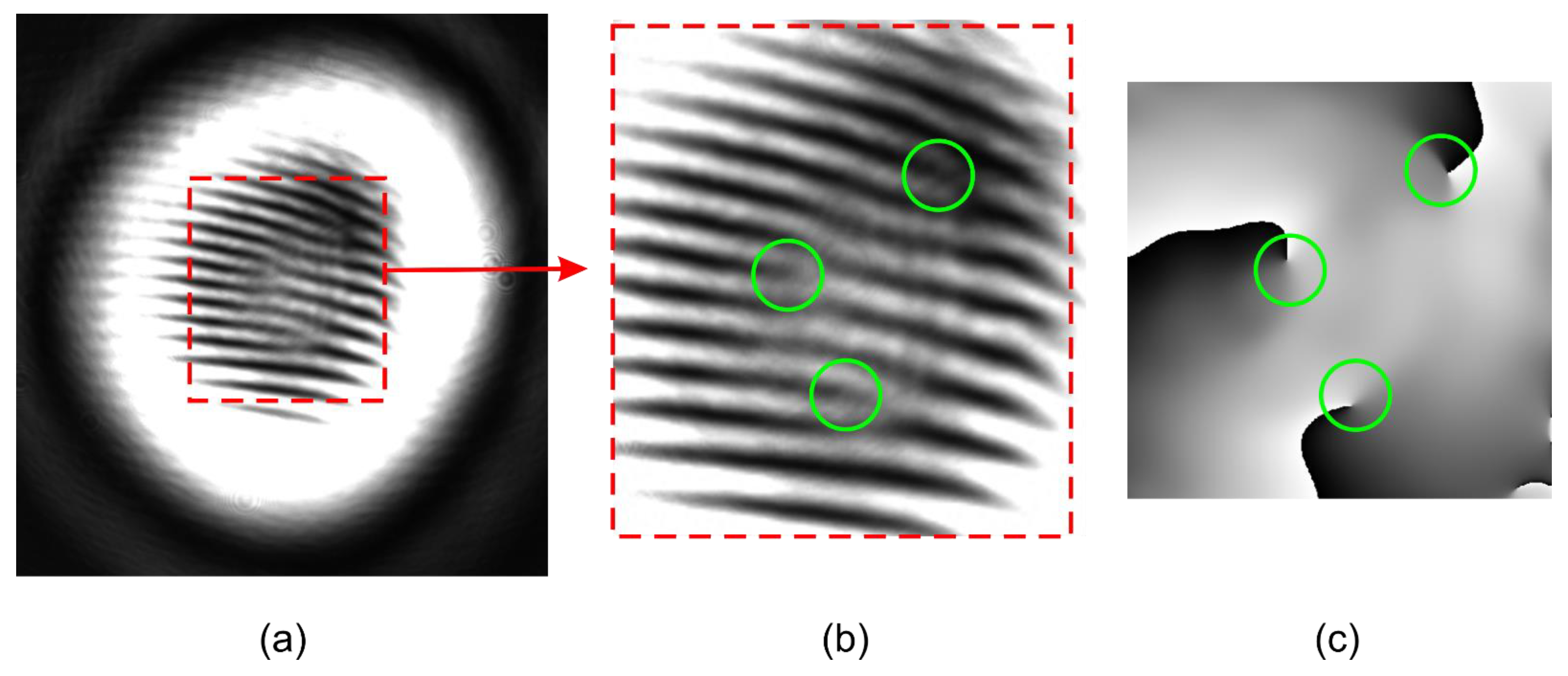
4. Method of Analyzing Interferograms with Fork Fringes

If we add a plane wave to the Laguerre–Gauss mode, we obtain interference patterns in which there is a characteristic bifurcation of the band called a fork. The bifurcation is in the place where the optical whirl occurs [32]. The bifurcation direction of the interference fringes depends on the sign of the TC. Figure 3 shows what the optical field distributions look like after adding a plane wave, in the case in which the optical vortices are separated. Two exemplary topological charges are shown. Additionally, phase maps for separated optical vortices with different TCs are presented. The values of charges and signs are different.

The recording of the fringe fields enables the standard Fourier technique [33] to be used for phase recovery. As mentioned before, vortex points are located at the beginning of the phase step line. This technique was used for experimental phase maps and gave correct results [34,35]. Alternatively, vortex points can be localized on phase maps with the use of the artificial neural network in the same way as in the pseudo-phase method (see next section).

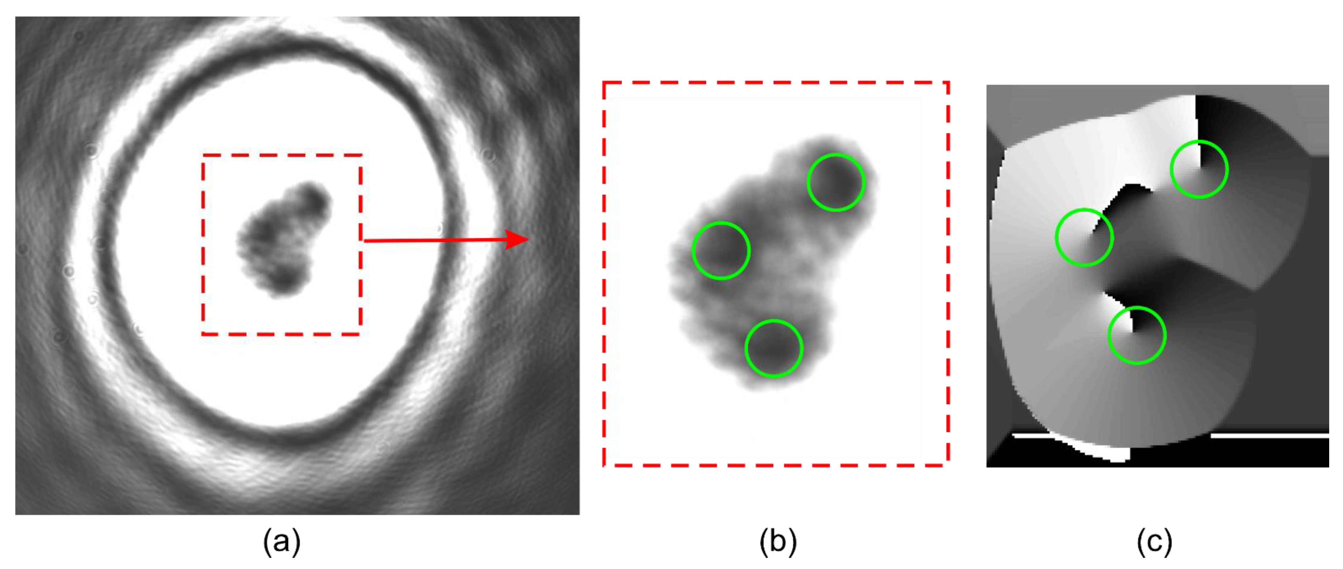
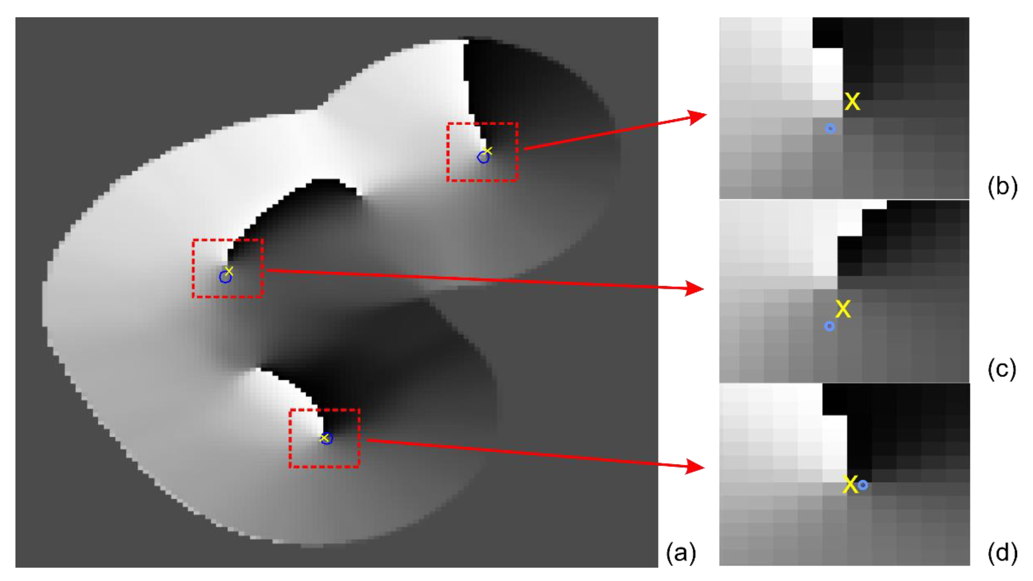
5. Pseudo-Phase Analysis Method

The spiral feature of the vortex beam can be extracted from the intensity images by applying the Laguerre–Gauss filter to obtain a so-called composite signal [36]. The recorded intensity is convolutional with the filter in the form of

$$fLG\left(r,\theta \right)=i·{\pi }^{0,2}{d}^{4}r\exp \left(-{\pi }^{0,2}{r}^2{d}^2\right)\exp \left(i·m\theta \right)$$

(3)

where r and θ are the polar coordinates, and d serves as a bandwidth of the LG filter.

The results obtained by the convolution can be generally written as

$$I_{con}\left(r,\theta \right)=I\left(r,\theta \right) ⨂ fLG\left(r,\theta \right)=\left|I_{con}\left(r,\theta \right)\right|\exp \left[i\phi \left(r,\theta \right)\right]$$

(4)

where φ(r, θ) is called the pseudo-phase.

Figure 4 shows the arguments and result (only phase φ) of the convolution operation of an LG filter with an intensity image. After performing the convolution operation described by Equation (4) and extracting the phase φ, we obtain the pseudo-phase maps shown in Figure 4c.

Colored and superimposed pseudo-phase and original phase maps are presented in Figure 5. Vortex positions are indicated by the red circles, which are at the point where the spiral connected with the 2π phase jump ends.

The presented pseudo-phase maps differ depending on the number of optical vortices. The next figure (Figure 6) shows an example for five optical vortices.

The initial location of vortex points can be determined from the intensity minima. Having defined these areas, we cut out small areas from the pseudo-phase maps around the initially found position. These maps contain the beginning of the phase jump. This phase jump line can be treated as an edge and can be extracted by the Roberts method [37] of edge finding, which is used in image processing. This method gives a location accuracy of 2 pixels on the CCD matrix. Location accuracy can be significantly increased by using a learned artificial neural network [38]. It is shown that the vortex can be localized with subpixel accuracy also on the experimental phase maps. A measurement accuracy on the order of 10⁻⁵ pixels was possible after the application of a feedforward artificial neural network technique with three hidden layers. The hidden layers had a hyperbolic tangent activation function, and the output layer was characterized by a linear activation function [39]. The close neighborhoods of vortex points on pseudo-phase maps are similar to the phase maps of the Laguerre–Gauss mode. Learned artificial neural networks work in the same way for both kinds of phase maps. Moreover, the algorithm based on neural networks is less sensitive to experimental disturbances related to wavefront noise.

6. Experimental Results

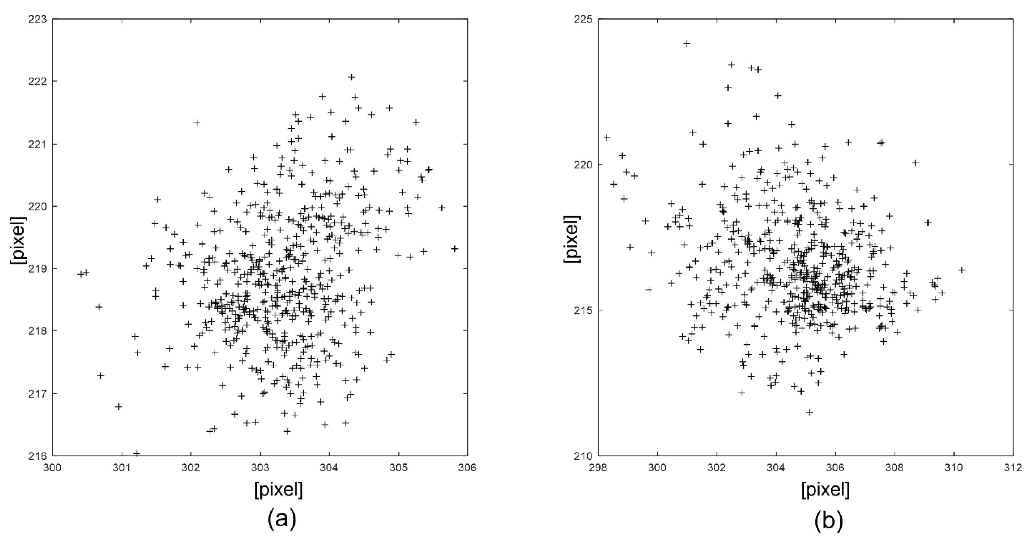
To verify the proposed solutions, measurements were made in the test system. The measuring system was set up so that only the intensity or the fringe field could be obtained. A stabilized He–Ne laser and an expander were used as the source. The measuring system was located in the room while the light beam went outside to the mirror and back; i.e., the influence of weather conditions was observed. The distance from the laser to the mirror was about 50 m, meaning that the optical path length was 100 m.

Figure 7 and Figure 8 show the measurement system, which was designed to verify if the proposed methods could be useful in a real situation. The configuration of the elements in both examples was the same, while the arrangement shown in Figure 8 shows the method of obscuring the reference wave responsible for the occurrence of bifurcated interference fringes. In such configurations, the system enables the recording of the intensity itself and the interference field.

Figure 9 and Figure 10 show the results of the experiment that were obtained in the configuration of the measurement system shown in Figure 7. Examples were selected with different fringes and different topological charges.

Locating the vortex points that are at the bifurcation of the fringes requires the following steps: notches for fringe field analysis and the application of the optical Fourier transform. Then, from the map of the diffraction spectrum, the first diffraction order should be selected, and the inverse Fourier transform should be applied to the next limited area (without the zero order). In this way, we obtained the complex distribution and, after calculating the angle, we obtained the phase maps shown in Figure 9c and Figure 10c. The jumps in the phase value appear on the obtained phase maps. It is important to find the ends of these lines, and image processing methods locate these ends with an accuracy not exceeding 1 pixel; to increase the accuracy of determining points, the authors used neural networks that analyzed selected regions with dimensions of 20 by 20 pixels, with the end of the phase jump line placed in the center of the cut area [34,35]. The learned artificial neural network locates vortex points with sub-pixel accuracy. For an algorithm based on neural networks, it makes no difference whether it looks for the end of the phase jump with phase or pseudo-phase maps. In both cases, the accuracies are the same.

In Figure 9 and Figure 10, the presence of vortex points is marked with green circles. It is possible to determine the location of optical vortices based on the bifurcation of the fringes, but these methods are not as accurate as the methods using phase fields. To locate bifurcations, one can also use algorithms based on neural networks. Information about the sign and topological charge of optical vortices can be easily read from the bifurcations of the interference fringes, while the localization itself is sensitive to noise and disturbances that occur during low-intensity recording.

Figure 11 shows an example of the images recorded in the configuration of the measurement arrangement shown in Figure 8. In this case, no additional light beam is needed. The recorded intensity for the three separated vortices was subjected to the convolution operation. As a result of convolution, the pseudo-phase maps shown in Figure 11c were obtained. This method is simpler in terms of technology and calculations than the fringe-field method, and the obtained result has the same accuracy.

In the measurement series, an exemplary measurement of which is shown in Figure 11, the minimization and pseudo-phase methods were used to locate vortex points. In half of the results, the minimum search method gave incorrect results due to turbulence. The pseudo-phase method worked properly on all captured images.

Figure 12 shows an example of the experimental results. There are three vortex points marked in the figure. In further calculations, the center of gravity of the figure formed by the constellation of optical vortices was determined. In this case, it was a triangle. The center of gravity is an appropriate point for beam positioning because communication often uses information carried by the optical vortices themselves.

If the disturbances do not affect the finding of the intensity minima, this method can be used for beam positioning. In experimental conditions, the intensities of the light beams are often distorted, which significantly affects the detection of a single beam. The pseudo-phase method gives more reliable results in non-laboratory conditions.

As an example, the results of tracking the centroid of a constellation of three optical vortices using the intensities recorded in two different settings of the measurement system (Figure 7 and Figure 8) are also shown (Figure 13).

Figure 13 shows the movement of an optical beam propagating through the air in free space. Both the pseudo-phase and interferogram methods allow the determination of the position of the center of gravity of the constellation of optical vortices. Figure 13 shows the location of approximately 500 points. The scatter of the results is due to atmospheric disturbances and ambient vibrations. The algorithms allowed us to track the position of the beam. Based on the information from the presented methods, it is possible to position the optical beam.

7. Discussion

The presented positioning methods use optical whirls as markers indicating the location of the beam center. Knowing the location of these tags enables effective positioning. Optical vortices are used as information carriers in optical communication. For this purpose, topological charges of OVs are sometimes recognized. The proposed methods can be used both for positioning and recognizing signs and topological charges. In measurements where the beam has passed through the air, the intensity distribution can be significantly distorted. In such cases, searching for vortex points based on the intensity minima is troublesome. The pseudo-phasic or phase field analysis method gives correct results under standard weather conditions. In addition, neural network algorithms applied to phase or pseudo-phase maps significantly improve positioning accuracy. The methods shown only analyze the center of the laser beam as the sensor aperture may be smaller than the beam aperture. An important aspect of the presented methods is the possibility to use only part of the optical beam for positioning.

References

1. Wang, J. Advances in communications using optical vortices. Photonics Res. 2016, 4, B14–B28. [Google Scholar] [CrossRef]
2. Richardson, D.; Fini, J.M.; Nelson, L.E. Space-division multiplexing in optical fibres. Nat. Photonics 2013, 7, 354–362. [Google Scholar] [CrossRef] [Green Version]
3. Li, G.; Bai, N.; Zhao, N.; Xia, C. Space-division multiplexing: The next frontier in optical communication. Adv. Opt. Photonics 2014, 6, 413–487. [Google Scholar] [CrossRef] [Green Version]
4. Gibson, G.; Courtial, J.; Padgett, M.; Vasnetsov, M.; Pas’Ko, V.; Barnett, S.; Franke-Arnold, S. Free-space information transfer using light beams carrying orbital angular momentum. Opt. Express 2004, 12, 5448–5456. [Google Scholar] [CrossRef] [PubMed] [Green Version]
5. Bozinovic, N.; Yue, Y.; Ren, Y.; Tur, M.; Kristensen, P.; Huang, H.; Willner, A.E.; Ramachandran, S. Terabit-Scale Orbital Angular Momentum Mode Division Multiplexing in Fibers. Science 2013, 340, 1545–1548. [Google Scholar] [CrossRef] [PubMed] [Green Version]
6. Wang, J.; Yang, J.-Y.; Fazal, I.M.; Ahmed, N.; Yan, Y.; Huang, H.; Ren, Y.; Yue, Y.; Dolinar, S.; Tur, M.; et al. Terabit free-space data transmission employing orbital angular momentum multiplexing. Nat. Photonics 2012, 6, 488–496. [Google Scholar] [CrossRef]
7. Willner, A.E.; Huang, H.; Yan, Y.; Ren, Y.; Ahmed, N.; Xie, G.; Bao, C.; Li, L.; Cao, Y.; Zhao, Z.; et al. Optical communications using orbital angular momentum beams. Adv. Opt. Photonics 2015, 7, 66–106. [Google Scholar] [CrossRef] [Green Version]
8. Yan, Y.; Xie, G.; Lavery, M.; Huang, H.; Ahmed, N.; Bao, C.; Ren, Y.; Cao, Y.; Li, L.; Zhao, Z.; et al. High-capacity millimetre-wave communications with orbital angular momentum multiplexing. Nat. Commun. 2014, 5, 4876. [Google Scholar] [CrossRef] [Green Version]
9. Li, L.; Zhang, R.; Zhao, Z.; Xie, G.; Liao, P.; Pang, K.; Song, H.; Liu, C.; Ren, Y.; Labroille, G.; et al. High-Capacity Free-Space Optical Communications Between a Ground Transmitter and a Ground Receiver via a UAV Using Multiplexing of Multiple Orbital-Angular-Momentum Beams. Sci. Rep. 2017, 7, 1–12. [Google Scholar] [CrossRef]
10. Krenn, M.; Handsteiner, J.; Fink, M.; Fickler, R.; Ursin, R.; Malik, M.; Zeilinger, A. Twisted light transmission over 143 km. Proc. Natl. Acad. Sci. USA 2016, 113, 13648–13653. [Google Scholar] [CrossRef] [Green Version]
11. Barreiro, J.T.; Wei, T.-C.; Kwiat, P.G. Erratum: Beating the channel capacity limit for linear photonic superdense coding. Nat. Phys. 2008, 4, 662. [Google Scholar] [CrossRef] [Green Version]
12. Molina-Terriza, G.; Torres, J.; Torner, L. Twisted photons. Nat. Phys. 2007, 3, 305–310. [Google Scholar] [CrossRef]
13. Vasnetsov, M.; Staliunas, K. (Eds.) Optical vortices. In Horizons in World Physics; Nova Science: New York, NY, USA, 1999; p. 288. [Google Scholar]
14. Gbur, G. Singular Optics; CRC Press: Boca Raton, FL, USA, 2017. [Google Scholar]
15. Allahyari, E.; Nivas, J.J.; Cardano, F.; Bruzzese, R.; Fittipaldi, R.; Marrucci, L.; Paparo, D.; Rubano, A.; Vecchione, A.; Amoruso, S. Simple method for the characterization of intense Laguerre-Gauss vector vortex beams. Appl. Phys. Lett. 2018, 112, 211103. [Google Scholar] [CrossRef]
16. Szatkowski, M.; Masajada, A.P.; Masajada, J. Optical vortex trajectory as a merit function for spatial light modulator correction. Opt. Lasers Eng. 2019, 118, 1–6. [Google Scholar] [CrossRef]
17. Kotlyar, V.V.; Kovalev, A.A.; Porfirev, A.P. Elliptic Gaussian optical vortices. Phys. Rev. A 2017, 95, 053805. [Google Scholar] [CrossRef]
18. Rozas, D.; Law, C.T.; Swartzlander, J.G.A. Propagation dynamics of optical vortices. J. Opt. Soc. Am. B 1997, 14, 3054–3065. [Google Scholar] [CrossRef]
19. Molina-Terriza, G.; Wright, E.; Torner, L. Propagation and control of noncanonical optical vortices. Opt. Lett. 2001, 26, 163–165. [Google Scholar] [CrossRef]
20. Ginzburg, V.L.; Pitaevskii, L.P. On the theory of superfluidity. Sov. Phys. JETP 1958, 34, 858–863. [Google Scholar]
21. Dennis, M.R.; Götte, J. Topological Aberration of Optical Vortex Beams: Determining Dielectric Interfaces by Optical Singularity Shifts. Phys. Rev. Lett. 2012, 109, 183903. [Google Scholar] [CrossRef] [PubMed]
22. Gan, X.; Zhang, P.; Liu, S.; Zheng, Y.; Zhao, J.; Chen, Z. Stabilization and breakup of optical vortices in presence of hybrid nonlinearity. Opt. Express 2009, 17, 23130–23136. [Google Scholar] [CrossRef] [PubMed]
23. Kumar, A.; Vaity, P.; Singh, R.P. Crafting the core asymmetry to lift the degeneracy of optical vortices. Opt. Express 2011, 19, 6182–6190. [Google Scholar] [CrossRef]
24. Bogatiryova, G.V.; Soskin, M.S. Detection and metrology of optical vortex helical wavefronts. SPQEO 2003, 6, 254–258. [Google Scholar] [CrossRef]
25. Frączek, W.; Frączek, E.; Mroczka, J. Experimental method for topological charge determination of optical vortices in a regular net. Opt. Eng. 2005, 44, 025601. [Google Scholar] [CrossRef]
26. Frączek, E.; Frączek, W.; Masajada, J. The new method of topological charge determination of optical vortices in the interference field of the optical vortex interferometer. Optik 2006, 117, 423–425. [Google Scholar] [CrossRef]
27. Kurzynowski, P.; Borwińska, M.; Masajada, J. Optical vortex sign determination using self-interference methods. Opt. Appl. 2010, XL, 165–175. [Google Scholar]
28. Malik, M.; Murugkar, S.; Leach, J.; Boyd, R.W. Measurement of the orbital-angular-momentum spectrum of fields with partial angular coherence using double-angular-slit interference. Phys. Rev. A 2012, 86, 063806. [Google Scholar] [CrossRef]
29. Chen, R.; Zhang, X.; Zhou, Y.; Ming, H.; Wang, A.; Zhan, Q. Detecting the topological charge of optical vortex beams using a sectorial screen. Appl. Opt. 2017, 56, 4868–4872. [Google Scholar] [CrossRef]
30. Gao, P.; Bai, L.; Wang, Z.; Wu, Z.; Guo, L. Evolution Behavior of Mixed Higher Order Optical Vortex–Edge Dislocations Propagating Through Atmospheric Turbulence. IEEE Photonics J. 2018, 10, 1–10. [Google Scholar] [CrossRef]
31. Hermosa, N.; Aiello, A.; Woerdman, J.P. Quadrant detector calibration for vortex beams. Opt. Lett. 2011, 36, 409–411. [Google Scholar] [CrossRef]
32. Aksenov, V.P.; Tikhomirova, O.V. Theory of singular-phase reconstruction for an optical speckle field in the turbulent atmosphere. J. Opt. Soc. Am. A 2002, 19, 345–355. [Google Scholar] [CrossRef]
33. Takeda, M. Spatial-carrier fringe-pattern analysis and its applications to precision interferometry and profilometry: An overview. Ind. Metrol. 1990, 1, 79–99. [Google Scholar] [CrossRef]
34. Popiołek-Masajada, A.; Masajada, J.; Szatkowski, M. Internal scanning method as unique imaging method of optical vortex scanning microscope. Opt. Lasers Eng. 2018, 105, 201–208. [Google Scholar] [CrossRef]
35. Frączek, E.; Popiołek-Masajada, A.; Szczepaniak, S. Characterization of the Vortex Beam by Fermat’s Spiral. Photonics 2020, 7, 102. [Google Scholar] [CrossRef]
36. Wang, W.; Yokozeki, T.; Ishijima, R.; Takeda, M.; Hanson, S.G. Optical vortex metrology based on the core structures of phase singularities in Laguerre-Gauss transform of a speckle pattern. Opt. Express 2006, 14, 10195–10206. [Google Scholar] [CrossRef]
37. Davis, L.S. A survey of edge detection techniques. Comput. Graph. Image Process. 1975, 4, 248–260. [Google Scholar] [CrossRef]
38. Frączek, E.; Idźkowski, B. Artificial Intelligent Methods for the Location of Vortex Points. In Transactions on Petri Nets and Other Models of Concurrency XV; Springer Science and Business Media LLC: Berlin/Heidelberg, Germany, 2020; Volume 12415, pp. 71–77. [Google Scholar]
39. Popiołek-Masajada, A.; Frączek, E.; Burnecka, E. Subpixel localization of optical vortices using artificial neural networks. Metrol. Meas. Syst. 2021, 28, 3. [Google Scholar] [CrossRef]
Figure 1. Vortex beam with a topological charge of m = 3: (a) intensity, (b) phase profile.
Applsci 11 07677 g001
Figure 2. Vortex beam with a topological charge of m = 3 after separation into three vortices with topological charges of m = 1: (a) intensity, (b) phase profile.
Applsci 11 07677 g002
Figure 3. The separated optical vortices with the addition of the plane wave, (a,c); the phase map for the separated optical vortices, (b,d). Cases (a,b) were generated for m = +3; (c,d) were generated for m = −5. The plane wave slope direction was the same in all cases.
Applsci 11 07677 g003
Figure 4. (a) Intensity of the vortex beam with a topological charge of m = 3 after separation into three vortices with topological charges of m = 1, (b) phase plotted as arg ( f L G ( r , θ ) ) , (c) pseudo-phase, plotted as arg ( I c o n ( r , θ ) ) for the vortex beam with a topological charge of m = 3. The figure shows the convolution operation.
Applsci 11 07677 g004
Figure 5. Pseudo-phase, plotted as arg ( I c o n ( r , θ ) ) for the vortex beam with a topological charge of m = 3 after separation into three vortices with topological charges of m = 1, with the original phase map colored and superimposed. The red circles indicate the locations of vortex points on both types of maps.
Applsci 11 07677 g005
Figure 6. (a) Intensity of the vortex beam with a topological charge of m = 5 after separation into five vortices with topological charges of m = 1, (b) pseudo-phase, plotted as arg ( I c o n ( r , θ ) ) with the original phase map colored and superimposed. The red circles indicate the locations of the vortex points on both types of maps.
Applsci 11 07677 g006
Figure 7. Diagram of an experimental setup for detecting an interferogram with fringes like a fork, BS—beam splitters, SPP—spiral phase plate.
Applsci 11 07677 g007
Figure 8. Diagram of an experimental system for detecting intensity with an additional shutter, BS—beam splitters, SPP—spiral phase plate.
Applsci 11 07677 g008
Figure 9. Experimental results with a separated optical vortex with the topological charge of m = 4. The intensity was recorded with an additional beam (Figure 7): (a) intensity, (b) magnified intensity area, (c) phase profile. The green circles represent the locations of the vortex points.
Applsci 11 07677 g009
Figure 10. Experimental results with a separated optical vortex with the topological charge of m = 3. The intensity recorded with an additional beam (Figure 7): (a) intensity, (b) magnified intensity area, (c) phase profile. The green circles represent the locations of the vortex points.
Applsci 11 07677 g010
Figure 11. Experimental results with a separated optical vortex with the topological charge of m = 3. Measurements made without an additional beam (Figure 8). (a) Intensity, (b) magnified intensity area, (c) pseudo-phase profile. The green circles represent the locations of the vortex points.
Applsci 11 07677 g011
Figure 12. Experimental results with a separated optical vortex with the topological charge of m = 3. (a) Pseudo-phase profile, (bd) enlarged fragments for three vortex points. The yellow “x” indicates a point found by the procedure using artificial neural networks, while the blue circle indicates the minimum intensity found on the basis of the procedure described in Section 3.
Applsci 11 07677 g012
Figure 13. Positions of the centroid of the three vortex point constellations (a) using the pseudo-phase method and (b) the bifurcated interference fringes method.
Applsci 11 07677 g013
Publisher’s Note: MDPI stays neutral with regard to jurisdictional claims in published maps and institutional affiliations.