Article

A Synthesized Study Based on Machine Learning Approaches for Rapid Classifying Earthquake Damage Grades to RC Buildings

1
Institute of Structural Mechanics (ISM), Bauhaus-Universität Weimar, 99423 Weimar, Germany
2
Research Group Theoretical Computer Science/Formal Methods, School of Electrical Engineering and Computer Science, Universität Kassel, Wilhelmshöher Allee 73, 34131 Kassel, Germany
*
Author to whom correspondence should be addressed.
Appl. Sci. 2021, 11(16), 7540; https://doi.org/10.3390/app11167540
Submission received: 30 July 2021 / Revised: 8 August 2021 / Accepted: 12 August 2021 / Published: 17 August 2021

Abstract

:
A vast number of existing buildings were constructed before the development and enforcement of seismic design codes, which run into the risk of being severely damaged under the action of seismic excitations. This poses not only a threat to the life of people but also affects the socio-economic stability in the affected area. Therefore, it is necessary to assess such buildings’ present vulnerability to make an educated decision regarding risk mitigation by seismic strengthening techniques such as retrofitting. However, it is economically and timely manner not feasible to inspect, repair, and augment every old building on an urban scale. As a result, a reliable rapid screening methods, namely Rapid Visual Screening (RVS), have garnered increasing interest among researchers and decision-makers alike. In this study, the effectiveness of five different Machine Learning (ML) techniques in vulnerability prediction applications have been investigated. The damage data of four different earthquakes from Ecuador, Haiti, Nepal, and South Korea, have been utilized to train and test the developed models. Eight performance modifiers have been implemented as variables with a supervised ML. The investigations on this paper illustrate that the assessed vulnerability classes by ML techniques were very close to the actual damage levels observed in the buildings.

1. Introduction

In seismic disturbances scenarios, the substandard performance of Reinforced Concrete (RC) frames has always been a crucial concern. Moreover, the massive occupancy of high-rise RC structures in urban areas and the migration of working professionals into metropolitan cities due to high-income propensity simply add to the residents’ and owners’ responsibilities and risks. It is imperative to identify the seismic deficiency in the structures and prioritize them for seismic strengthening. Application of rigorous structural analysis methods for studying the seismic behavior of buildings is impractical in terms of computing time and cost, dealing with a large building stock, a quick assessment, and a reliable method to adapt corrective retrofitting methods for deficient structures. RVS is more widely known for fundamental computations; a rapid and reliable method used to assess seismic vulnerability. RVS was developed initially by the Applied Technology Council in the 1980s (U.S.A.) to benefit a broad audience, including building officials, structural engineering consultants, inspectors, and property owners. This method was designed to serve as the preliminary screening phase in a multi-step process of a detailed seismic vulnerability assessment. The procedure is classified typically as a three-stage process, wherein the first phase consists of performing a rapid visual screening process. The structures which fail to satisfy the cutoff scores in the first step shall be subjected to a stage two and three detailed seismic structural analysis performed by a seismic design professional. The process of RVS was developed based on a walk-down survey for physical assessment of the buildings from the exterior, and, if possible, from the interior for identifying the primary structural load resisting system. A trained evaluator performs the walk-down survey for recording the predefined parameters from the structures. The survey outcome grades the buildings based on basic computations and compares them to a predefined cut-off score. If the building has scored more than the cut-off score, it can be termed seismically resistant and safe. On the contrary, the structure shall be subjected to detailed investigation. Therefore, we can recognize now the need for research contributions in the RVS procedure to make it as easy and as reliable as possible.
RVS has been adopted widely in various countries globally, especially in the United States, with several guidelines from the Federal Emergency Management Agency (FEMA) for seismic vulnerability and rehabilitation of structures. The first edition was published in 1989 with revisions in 1992, 1998, and 2002 (FEMA 154) [1]. The RVS procedure has been modified by many researchers, such as the application of fuzzy logic and artificial neural networks (ANN). Trained fuzzy logic application in RVS shows a marked improvement in the performance of the standard procedure [2]. Furthermore, the logarithmic relationship between the final obtained scores and the probability of collapse at the maximum considered earthquake (MCE) makes the results difficult. Yadollahi et al. [3] proposed a non-logarithmic approach after identifying this limitation, especially from the perspective of project managers and decision-makers, who shall be able to interpret the results readily. Yang and Goettel [4] have developed an augmented approach to RVS called E-EVS by using the RVS scores for the initial prioritization of public educational buildings in Oregon, USA. However, the RVS method has been developed and used in different countries like Turkey, Greece, Canada, Japan, New Zealand, and India with local parametric variations depending on the construction method, structural materials used, the structural design philosophies, and the seismic hazard zones [5].

Background of Study

The RVS approach has been used to determine the structural damage states and index of the affected buildings [6,7]. The FEMA in the United States identified the demand for a rapid, reliable, and non-rigorous method for damage state classification in 1988 [1]. The fundamental method (1988) was later subjected to revisions in 2002 to incorporate the latest research advancements in seismic engineering. A highly relevant and adequate explanation of this approach has been presented in the research by Sinha and Goyal [8]. This approach was further adopted by various countries across the globe for damage state characterization [2] with adequate customization in the method according to country-specific materials, methods, and design philosophies in construction—for example, Indian RVS approach (IITK-GSDMA) [9]. RVS is highly effective in analyzing a large building stock due to rapid computational time and non-rigorous methodology. Seismic vulnerability assessment (SVA) is performed mainly in three stages [10]: walk-down evaluation, preliminary evaluation, and detailed evaluation. The SVA approach’s primary component begins with the physical presence of the trained evaluator with the respective data sheets onsite by performing a walk-down survey to record the seismic parameters of the structure. In many instances, the evaluator needs to enter and have access to the building; architectural moldings hide the structural members for aesthetic purposes. The structures that struggle to fulfill the expectations shall be subjected to the second stage. The second stage comprises a more detailed and extensive analysis in which seismic aspects to different structural characteristics such as the actual ground conditions, the consistency of the material, the condition of building elements, etc. shall be considered. If found to be necessary, the structure shall be subjected to the final stage, where a more detailed and rigorous analysis is used. In this stage, an in-depth and profound nonlinear dynamic analysis and research of the building’s seismic response shall be studied, which shall also help to optimize the application of seismic strengthening techniques on the structure [11]. The RVS is a scoring-based approach, wherein performing some elementary computations result in the final performance score for predicting the damage state classification of that structure. Every RVS approach from different countries has its predefined cutoff scores.
Extensive research has been published to integrate scientific methods from several domains to blend them into the scope of RVS and propose a smarter resultant approach; for instance, statistical methods [12,13], ANN and ML techniques [14,15,16,17,18,19,20], multi-criteria decision-making [5,21], deep learning classification [22], and type-1 [23,24,25,26] and type-2 [27,28] fuzzy logic systems. Within the framework of statistical methodology and regression analysis, multiple linear regression analysis [12] is the most commonly used technique for damage state classification in the RVS domain [2], preceded by other approaches such as discriminant analysis proposed in [29]. Morfidis and Kostinakis [30] have investigated the application of seismic parameter selection algorithms by choosing the optimum number of seismic parameters that can upgrade the performance of the RVS. Furthermore, Jain et al. have proved the integrated use of various interesting variable selection techniques such as R 2 adjusted, forward selection, backward elimination, and Akaike’s and Bayesian information criteria [31]. Furthermore, in the research proposed in [32], the traditional least square regression analysis and multivariate linear regression analysis were used. Askan and Yucemen [33] suggested several probabilistic models, such as models based on reliability and “best estimate” matrices of the likelihood of damage for a different seismic zone by combining expert opinion and the damage statistics of past earthquakes. Morfidis and Kostinakis [34] have explicitly proved that ANN could be practically applied in RVS from an innovative perspective, carried forward by the pioneering application of the coupling of fuzzy logic and ANN’s by Dristos [35]. In this research, untrained fuzzy logic procedures have shown exceptional performance. Even so, the RVS procedures adopted presently are largely dependent on the evaluator’s perspective, errors, and uncertainties or the crude assumption of linear dependency in seismic parameters. ML, a subdivision of artificial intelligence, allows highly efficient computing algorithms with training and learning for instinctive development. It aims to make forecasts using data analysis software. The ML algorithms typically include three necessary components: description, estimation, and optimization.
The domain of the study contained multi-class classification problems that require multi-class classification techniques of ML. Tesfamariam and Liu [19] conducted a study using eight different statistical techniques, such as K-Nearest Neighbours, Fisher’s linear discriminant analysis, partial least squares discriminant analysis, neural networks, Random Forest (RF), Support Vector Machine (SVM), Naive Bayes, and classification tree, to assess the seismic risk of the reinforced buildings while using six feature parameters. Extra Tree (ET) and RF performed better than the others, and the authors suggested further investigation and calibration of the result using more feature vectors and big datasets.
The study conducted by Han Sun [36] has emphasized various machine learning applications for building structural design and performance assessment (SDPA) by reviewing Linear Regression, Kernel Regression, Tree-Based Algorithms, Logical Regression, Support Vector Machine, K-Nearest Neighbors, and Neural Network. The previous achievements in the field of SDPA are categorized and reviewed into four sections: (1) anticipation of structural performance and response, (2) clarifying the experimental data and creating models to forecast the component-level structural properties, (3) data recovery from texts and images, and (4) pattern identification in data from structural health monitoring. The authors have also addressed the challenges in practicing ML in building SDPA.
In another study performed by Harirchian et al. [37], SVM performed comparatively efficient even in the case of many features. Kernel trick is one of SVM’s strengths that blends all the knowledge required for the learning algorithm, specifying a key component in the transformed field [38].
This work’s focus includes demonstrating and utilizing a multi-class classification of ML techniques for preliminary supervised learning datasets. Quality and quantity of data for supervised machine learning models play a significant role in achieving a high yield working model. Focusing on this, accurate post event data are collected from four separate earthquakes, including Ecuador, Haiti, Nepal, and South Korea. The issue of data shortage is crucial as data are the building blocks of ML models. Out of several supervised learning models, the authors have selected five influential algorithms: SVM, K-Nearest Neighbor (KNN), Bagging, RF, and Extra Tree Ensemble (ETE). Finally, the research demonstrates the feasibility of the proposed ETE model and the detailed analysis of the earthquake results.

2. Background of the Selected Earthquakes

The study of structures affected by the Ecuador, Haiti, Nepal, and South Korean earthquakes has been supplemented by the data archived in the open-access database of the Datacenterhub platform [39], along with the data collected from the investigations by different research groups on that platform [40,41,42,43].
In this particular study, the earthquake in Ecuador that occurred on 16 April 2016, has been considered, which additionally caused a tsunami, primarily affecting the coastal zone of Manabí. The catastrophic earthquake and tsunami had resulted in widespread devastation of infrastructure, with around 663 deaths [44]. The American Concrete Institute (ACI) research team, in collaboration with the technical staff and students of the Escuela Superior Politécnica del Litoral (ESPOL), performed a detailed survey to generate a memorandum of damaged RC structures affected due to the earthquake [41]. The earthquake data have been recorded at stations placed primarily upon two different soil profiles, namely APO1, the IGN strong-motion station’s location, and Los Tamarindos. APO1 consists of both alluvial soils with an average shear wave velocity at the height of 30 m, Vs30 of 240 m/s, while Los Tamarindos consist of alluvial clay and silt deposits with a Vs30 of 220 m/s [45].
The Haiti earthquake, which occurred on 12 January 2010, has been considered for this assessment. Seismologists from the University of Purdue, Washington University, and Kansas University, in cooperation with research workers from Université d’Etat d’Haïti, had surveyed and compiled the data of 145 RC buildings that had been affected by the earthquake [46]. The data had been collected meticulously from the southern and northern plain of Léogâne city, west of Port-au-Prince, where the structural damage was the most severe. In the affected region, soil properties indicate granular alluvial fans and soft clay soils, respectively [47]. The ShakeMap of the U.S. Geological Survey indicates the ground motion at Léogâne having an intensity of IX and Port-au-Prince having intensity VIII [48].
Moreover, another devastating earthquake that has also been assessed in the current study is the Nepal Earthquake in May 2015. This earthquake caused massive devastation of the land and supplementary, long-term effects such as the resultant landslides of the earthquake continuing to pose immediate and long-term hazards to the affected area’s life and infrastructure [49]. Surveys conducted by the researchers from Purdue University and Nagoya Institute of Technology in association with the ACI resulted in collecting and compiling data of damage of 135 low-rise reinforced concrete buildings with or without masonry infill walls [43]. The Kathmandu valley has a soil profile consisting primarily a heterogeneous mixture of clays, sands, and silts with thicknesses ranging up to nearly 400 m [50]. The U.S. Geological Survey ShakeMap recorded a ground motion intensity of VIII, with the epicenter being 19 Km to the South-East of Kodari. It has been investigated that the site-specific design spectrum and ground motion intensity have a significant effect on the performance of the building’s parameters against earthquakes [51].
Finally, the last earthquake considered in the study occurred in Pohang, South Korea on 15 November 2017. It is assumed that this earthquake was not a naturally occurring event but was influenced and triggered by various industrial activities. Furthermore, this earthquake has potentially increased the area’s seismic vulnerability by stressing the fault lines in the vicinity [52]. Two megacities of Huenghae and Pohang have observed a considerable impact in terms of structural and social. The economy was affected significantly, with losses amounting to around 100 million US dollars in the public and private infrastructures. A team of researchers from ACI conducted the damage data collection in collaboration with multiple universities and research institutes [40]. The subsurface soil strata show the integration of filling, alluvial soil, weathered soil, weathered rock, and bedrock. The U.S. Geological Survey ShakeMap recorded a ground motion intensity of VII [53]. A ShakeMap depicts the intensity of ground shaking produced by an earthquake. ShakeMaps provide near-real-time maps of ground motion and shaking intensity for seismic events. Figure 1 shows the Macroseismic Intensity Maps (ShakeMap) and Modified Mercalli scale (MM) for the selected earthquakes. Such maps are generated based on shaking parameters from integrated seismographic networks locations, and combined with predicted ground motions in places where inadequate data are collected. Finally, it released electronically within minutes of the earthquake’s occurrence, whenever changes that occur in the available information maps are updated.
Since peak ground acceleration and peak ground velocity of earthquakes are important and useful to assess seismic vulnerability and risk on buildings [54], Figure 2 indicates the properties of selected earthquakes that have been recorded. As the earthquakes in the selected regions were significantly strong, it has been considered as the MCE in this study.

Choice of Building’s Damage Inducing Parameters

Past contemplation and acknowledgment of the seismic event are essential requirements while performing any RVS study. Many authors have utilized different characteristics of buildings in their research work to assess the seismic vulnerability [3,21,32,60,61,62]. FEMA154 [1], as a literature review, explicitly states the most useful inputs, such as system type, vertical irregularity, plan irregularity, year of construction, and construction quality. Yakut et al. [63] have suggested a range of additional and significant structural parameters for evaluating building vulnerability, which indicate damage to buildings and should apply for potential research purposes. In this study, the parameters are the same as the basis of the Priority Index that have been proposed by Hasan and Sozen [64]. The eight parameters are namely No. of story, total floor area, column area, concrete wall area in X and Y directions, masonry wall area in X and Y directions, and existence of captive columns (or short columns) such as any semi-infill frames, windows of partially buried basements, or mid-story beams lead to captive columns. The featured parameters have been presented in Table 1.

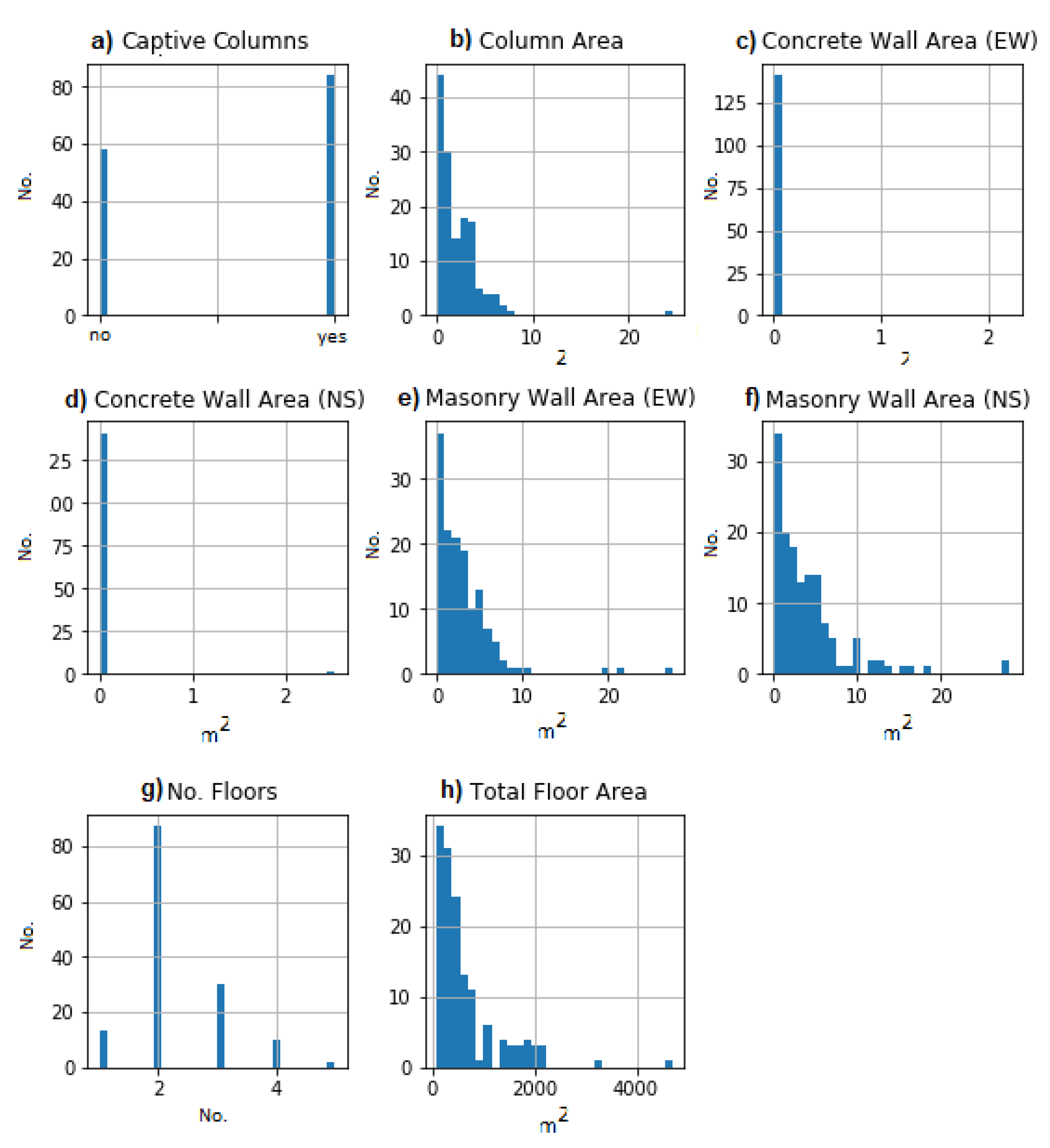
3. Input Data Interpretations

Derived from artificial intelligence, ML teaches computers to think and make decisions like humans where they can learn and improve upon past their experiences. ML can automate most of the works that are data-driven or defined by a set of rules. The learning patterns in ML are widely divided into three sub-classes: Supervised Learning, Unsupervised Learning, and Reinforced Learning. The collection of the dataset for training the ML model for this study contains multi-class labeled data. Therefore, the data analysis is applied using some of the popular ML supervised learning algorithms.
The base of ML predictive models is the training data used to teach the machines to identify different patterns. The concept of machine learning is ineffective without quantitative data, but only quality data can build an efficient model.
There are various categories in which the data can be presented, such as categorical, numerical, and ordinal. ML predicts better with numerical data. For most of the cases where the dataset contains non-numerical values, the data are transformed into their respective numerical form using specific methods available in ML libraries, such as One-Hot-Encoding and Label-Encoder from sciKit-learn library. The following study incorporates data in numerical form and is collected from four different seismic crisis.
In this section, the input data are interpreted based on their damage scale and are assigned under a specific damage scale. Table 2 presents the number of buildings for each earthquake’s dataset and the pie-charts demonstrated together in Figure 3 show the distributions of earthquake affected building samples for Ecuador, Haiti, Nepal, and Pohang to the respective damage scale. Most of the buildings came under grade 3. The moderate magnitude of earthquake resulted in the least number of affected buildings in Pohang.
Table 3 describes the damage severity of the damage scales for selected earthquakes. Though the scaling is not the same in all the earthquake cases, the associated risk is uniformly distributed with varying grades.
The seismic damages are evaluated using eight different input parameters drawn from the sample buildings. Figure 4, Figure 5, Figure 6 and Figure 7 are the histograms plotted for Ecuador, Haiti, Nepal, and Pohang, respectively, to analyze the distribution of the input parameters. In each histogram, the y-axis symbolizes the number of counts or the frequency, and the x-axis represents the corresponding feature parameter from every dataset. For Ecuador, as it is shown in Figure 4a–h, (b) Column Area, (e) Masonry Wall Area (EW), (f) Masonry Wall Area (NS), (g) No. of Floor, and (h) Total Floor Area show Gaussian distribution, whereas (a) Captive Columns appear to have a bimodal distribution. The absence of data are visible for (c) Concrete Wall Area (EW) and (d) Concrete Wall Area (NS).
Figure 5a–h represents data from Haiti. It shows the exponential distribution for the (b) Column Area, (e) Masonry Wall Area (EW), (f) Masonry Wall Area (NS), (g) No. of Floor, and (h) Total Floor Area, respectively. It can be concluded that there is no linear distribution of parameters. (a) Captive Columns have a bimodal distribution. For Nepal in Figure 6a–h, it gives Gaussian distribution for the (b) Column Area, (g) No. Floors, (h) Total Floor Area, and (f) Masonry Wall Area (NS), whereas the distribution pattern for (e) Masonry Wall Area (EW) is exponential. (a) Captive Columns is bimodal, and there is no data to show for (c) Concrete Wall Area (EW), (d) Concrete Wall Area (NS).
The data distribution for Pohang in Figure 7a–h; it is visible that Pohang has very little sample data in the dataset. The (b) Column Area represents a Gaussian distribution over the data, whereas the (c) Concrete Wall Area (EW), (d) Concrete Wall Area (NS) and (h) Total Floor Area are distributed exponentially. (e) Masonry Wall Area (EW) and (f) Masonry Wall Area (NS) clearly shows the absence of any data.

4. Supervised Learning as Statistical Analysis for RVS

Supervised Learning [65] for multi-class classification has several learning methods. In this study, five different ML algorithms are applied, such as SVM, KNN, Bagging, RF, and ETE to the input datasets to examine the most suitable classifier based on accuracy.

4.1. Support Vector Machine

An SVM [66] is a powerful and flexible model in ML. It performs well in linear, nonlinear classification and regression problems and also for outlier detection. SVM’s foundation is built over linear classification problems, primarily for separating two distinct classes using decision boundaries created by the support vectors [67]. Often hyperparameter c is tuned to regularize the over-fitting of the SVM model. By transforming the input space into a higher dimension, SVM can easily fit for polynomial features, often called as kernel trick. The following list shows the most popular polynomial kernels used for nonlinear as well as multi-feature classification problems:
  • Linear: K ( a , b ) = a T · b ;
  • Polynomial: K ( a , b ) = ( γ a T · b + r ) d ;
  • Gaussian RBF: K ( a , b ) = e x p ( γ | | a b | | 2 ) ;
  • Sigmoid: K ( a , b ) = t a n h ( γ a T · b + r ) ;
where
  • K: kernel;
  • d: degree of polynomial;
  • a and b: vectors in the input space ∈ I R ;
  • γ : mapping function;
  • r: an independent parameter, such that r ≥ 0.
With an increase in the complexity of the Kernels, the computational time for the classifier also increases. Linear Kernel SVC is comparatively faster among the rest of the kernels and fits well for more massive data. In the case of nonlinear and complex data, Gaussian RBF works fast.

4.2. K-Nearest Neighbor

Proposed by Evelyn Fix [68] in 1951 and further modified by Thomas Cover [69], K-nearest neighbor, or KNN, is ML’s simple non-parametric procedure used for classification and regression problems. It presumes that the same class data stay close to each other, and the data are assigned to a particular class with the maximum vote by its neighbors. It is also known for lazy learning as the classification is locally approximated. Distance functions (listed below) play an essential role in the algorithm; therefore, the classification accuracy is improved when it is standardized or normalized.
  • Euclidean: ( n = 1 k ( x i y i ) 2 );
  • Manhattan: ( n = 1 k | x i y i | );
  • Minkowski: ( n = 1 k ( | x i y i | ) q ) 1 / q .
where
  • x i is the ith value of x and y i is the ith value of y ,
  • k is the number of nearest neighbors, and
  • q is a positive value.

4.3. Bootstrap Aggregation/Bagging

Leo Breiman proposed bootstrap Aggregation (or Bagging) in 1996 [70]. Bagging can be considered as a specific instance belonging to the family of ensemble methods [71]. These methods notably bring randomization to the learning algorithm or exploit at each run a different randomized version of the original learning sample to generate robust, diversified ensemble models with lower variance. By aggregating the predictions from all the classifiers, the final accuracy is evaluated. Bagging draws randomization by creating the models from bootstrap samples built-in subsets from replacing the original dataset.

4.4. Random Forest

RF is an ensemble classifier and a significant advancement in the decision tree in terms of variance. The idea was proposed by Leo Breiman [72] with combined concepts of Bagging [70] and random feature selection by Ho [73,74] and Amit and Geman [75,76]. Randomly selected subsets (i.e., a bootstrapped sample) of training data form multiple numbers of trees that go under evaluation independently. The probability of each tree is considered, and the average is calculated for all the trees and then decides the class of the sample. RF classifier merges the concepts of bagging and random feature subspace selection to build stable and robust models. It performs better than simple trees in terms of the overfitting of data.

4.5. Extra Tree

Various generic randomization methodology like Bagging has been proposed [74,77,78], which have been proven for better accuracy when compared to other supervised learning classifiers like SVM. Ensemble methods, in combination with trees, provided low computational cost and high computational efficiency. Several studies focused on specific randomization techniques for trees based on direct randomization methods for growing trees [71].
ET or Extremely Randomised Trees is also an ensemble learning approach and fundamentally based on Random Forest. ET can be implemented as ExtraTreeRegressor as well as ExtraTreeClassifier. Both methods hold similar arguments and operate similarly, except that ExtraTreeRegressor relies on predictions made by the tress’s aggregated predictions, and ExtraTreeClassifier focuses on the predictions generated by the majority voting from the trees. ExtraTreeClassifier forms multiple unpruned trees [79] from the training data subsets based on the classical top-down methodology. Compared to other tree-based ensemble methods, the two significant differences are that ET splits the nodes by selecting the cut-points randomly and thoroughly. Moreover, it utilizes the complete learning sample (rather than a bootstrap replica) to build the trees.
The prediction for the sample data makes the majority of the voting. While implementing ML algorithms that utilize a stochastic learning algorithm, it is recommended to assess them using k-fold cross-validation or merely aggregate the models’ performance across multiple runs. To fit the final model, few hyperparameters can be tuned, like increasing the number of trees and the number of samples in a node, until the model’s variance reduces across repeated evaluations. The ET classifier has low variance and has higher performance with noisy features as well.

5. Data Analysis and Method Implementation

This section discusses the available datasets and implements different ML techniques to verify their predictive accuracy against the unseen test examples. Figure 8 shows the different stages of the methodology implemented to build the ML classifiers. Each of the four stages exhibits the necessary steps connected from data pre-processing to creating the complete ML model. They are further elaborated in the below sections.

5.1. First Stage: Data Pre-Processing

Data pre-processing plays an essential part in machine learning as the quality of the information extracted from the data are responsible for affecting the model’s learning quality and capacity. Therefore, pre-processing the data is crucial before feeding it to the algorithm for training, validation, and testing purposes.
In general, raw datasets may contain missing feature points, disorganized data, and imbalanced input feature points over the attributes. For optimum accuracy, datasets are pre-processed, which includes handling the missing values, standardizing the data, and balancing the imbalanced distribution of feature points. An imbalanced dataset contained an uneven number of input examples for the output classes. The study utilizes Python programming language, which has inbuilt libraries such as NumPy, sklearn, matplotlib, which support ML algorithms strongly. Furthermore, the libraries offer different classes and methods responsible for performing different tasks for the provided datasets.
The datasets used in the study include the data collected from four different earthquakes, which occurred in Ecuador, Haiti, Nepal, and Pohang. Haiti’s dataset contains few missing values, whereas all the datasets show the disproportionate distribution of feature points over all the eight input parameters. For Haiti, the missing values are replaced with the attribute column’s respective mean value using the SimpleImputer class from Python’s sklearn library. SimpleImputer verifies the missing values; if so, it replaces the missing value using the mean/median/most frequent/constant value from the respective column. Standardization of the data is performed by MinMaxScaler class from the sklearn library, which helps to scale the feature points between range 0 and 1. Imbalanced categorization acts as an objection for predictive modeling as most of the machine learning algorithms applied for classification are created around the idea of an equal number of examples for each category class. For balancing the feature point distribution over the different classes, the over-sampling technique of SMOTE [80] method is used. It creates synthetic samples for the minority class, hence making a balance with the majority class.
Subsequently, the dataset splits into two subsets, a training set with 80% data and testing sets with 20% data. Splitting of data in ML is significant, where the hold-out cross-validation ensures generalization to ensure that the model is accurately interpreting the unseen data [81].

5.2. Second Stage: Model Evaluation

ML classifier is designed to predict the unseen data. ML models can perform the various required actions; it is essential to feed them the training subsets, followed by the validation subsets, ensuring that the model interprets the correct data. A significant and relevant dataset can help the ML model to learn faster and better. As mentioned in the earlier section, there are five candidate algorithms with which the models are trained and fit, namely SVM, KNN, Bagging, RF, and ET. Using the RepeatedStratifiedKFold class from the scikit learn library, the models are trained to be not too optimistically biased and catch the selected model’s variance.
Model performance can be influenced by two configuration factors: parameter and hyperparameter. Parameters are the internal configuration variable and are often included as a part of the learning model. They help the model in making predictions and can characterize the model’s skill for the given problem. In general, parameters can not be set manually; instead, they are saved as a part of historical learned models.
Hyperparameters can be configured externally (often set heuristically) and are tuned based on the predictive model user has selected for solving the problem. Hyperparameters help estimate the model parameters, and the user often searches for the best hyperparameter by tuning the values using methods like grid search or random search available in scikit learn library.
For the study, all the models are created using the default hyperparameters for their respective algorithms. While examining the models, the mean and standard deviation values of predictive accuracy are observed at each iteration. Every algorithm’s efficiency is analyzed based on the highest achieved predictive accuracy for the unseen test data. Figure 9 represents the candidate algorithms’ predictive accuracy for each of the respective datasets. The observed results suggest that ET performs best on the given datasets while classifying the unseen test data; the overall accuracy is 64%, 63%, 72%, and 67% for Ecuador, Haiti, Nepal, and Pohang, respectively. ET and RF have performed better at predicting test data in comparison to the rest of the ML techniques.

5.3. Third Stage: Model Selection and Visualization

Based on the candidate classifiers’ evaluation result, ET has above average performance with each of the input datasets, and therefore ExtraTreeClassifier is explored further in the study to visualize the accuracy results.
Visualization techniques such as Confusion Matrix and ROCAUC plots are used to show the efficiency of ET clearly. Confusion matrix or error matrix summarize the classifier’s performance [82] by comparing the predicted value with the actual value, presented in a [nxn] matrix, where n is the number of classes in the data. The structure of this matrix is shown in Figure 10, and it serves as a basis for calculating several accuracy metrics.
A recall is the ratio of true positives to the sum of true positives and false negatives (damage misclassified as non-relevant), while Precision illustrates the proportion of correctly classified instances that are relevant (called true positives and defined here as recognized damage) to the sum of true positives and false positives (damage misclassified as relevant). In our case, false positives and false negatives are represented by damage grades recognized as higher or fewer damage grades, respectively. Each of the presented confusion matrices in this study provides the accuracy of each damage scale by each RVS method and provides information such as recall (true positive rate) and precision (positive prediction value) calculated from the below equations:
Precision = T P T P + F P
Recall = T P T P + F N
Accuracy = T P + T N T P + T N + F P + F N
The Receiver Operating Characteristic/Area Under the Curve or ROCAUC plot estimates the classifier’s predictive quality and compares it to visualizes the trade-off between the model’s sensitivity and the specificity. The true positive and false positive rates are represented by the y-axis and x-axis, respectively, in the plots. Typically, ROCAUC curves are used to classify binary data to analyze the output of any ML model. As this study is conducted for a multi-class classification problem (multiple damage scales), Yellowbrick is used for visualizing the ROCAUC plot. Yellowbrick is an API from scikit learn to facilitate the visual analysis and diagnostics related to machine learning.
Furthermore, the value of micro-average area under the curve (AUC) is the average of the contributions of all the classes AUC value, whereas the macro-average is computed independently for each class and then aggregate (treating all classes equally). For multi-class classification problems, micro-average is preferable in case of an imbalanced number of input examples for each class. For this study, since all the classes are balanced with equal input data, the micro and macro average value is almost identical.
Figure 11, Figure 12, Figure 13 and Figure 14 illustrate how well the ET ensemble technique worked overall with each dataset. The confusion matrix presented in Figure 11a and it shows the model’s efficiency in predicting test examples related to each class, and Figure 11b is the corresponding ROCAUC plot and similar respective results for the AUC are produced and it applies to other related figures. Figure 11 represents the confusion matrix for Ecuador that anticipates the classifier’s prediction accuracy; class 1 has maximum correct predictions, whereas performance for class 2 is least. Figure 11b depicts the ROCAUC plot for the test data, and the curves show that the model fits with the unlabeled data sufficiently. Class 1 (AUC = 0.89) clearly shows that the test data belonging to the class are well predicted. The high value of AUC signifies a better predicting model. Class 1 has the highest AUC values, whereas class 3 has the lowest among all.
For Haiti, the confusion matrix in Figure 12a shows that class 2 has the maximum correct predictions for the unseen test data, and class 3 has the least correct predictions. The ROCAUC plot in Figure 12b also depicts the highest value for class 2. The micro and average macro value for the classes are nearly the same. The same pattern can be seen in the AUC values, with the minimum value for class 3 (0.73) and maximum for class 2 (0.94).
Nepal and Pohang have a 4 × 4 matrix, based on their number of damage scale. Confusion matrix for Nepal in Figure 13a has class 3 with the correct predictions and maximum for class 1. The AUC value for class 3 in Figure 13b is the maximum. The micro and macro-average values of AUC for all the classes are 0.97 and 0.96, respectively.
In the confusion matrix result for Pohang, Figure 14a illustrates that class 1 has the maximum correctly predicted test examples, and a similar pattern is visible for the AUC value in Figure 14b, with class 1 having a maximum AUC value. The micro and macro value for all the classes are 0.74 and 0.76, respectively. Insufficient data for Pohang resulted in several zero values in the confusion matrix. Overall, while predicting the test set, Nepal has attained the highest accuracy of 72% out of all the datasets.

5.4. Fourth Stage: Hyper-Parameter Optimization and Model Fitting

After selecting ET as the most suitable classifier and visualizing its performance with all datasets, the final stage is to tune its relevant hyperparameters and check the model performance with each dataset to compare with the results before and after tuning the hyperparameters.
As mentioned in the previous section, a hyperparameter is a factor whose value dominates the learning process. These hyperparameters are to be set before executing a machine learning algorithm, unlike model parameters that are not fixed before execution; instead, they are optimized during the algorithm’s training. These factors or parameters are tunable and can openly affect how well model trains. Hyperparameters may impact directly on the training of ML algorithms. Thus, to achieve maximal performance, it is essential to understand how to select and optimize them [83]. The study includes optimizing three important ET hyperparameters (listed below), and each classifier is configured based on them.
  • Number of Trees: One of the critical hyperparameters for the ET classifier is the number of trees that the ensemble holds, represented by the argument “n_estimator” ExtraTreeClassifier. In general, the number of trees increases until the performance of the model stabilizes. A high number of trees may lead to overfitting and a slowing down of the learning process, but the unlikely ET algorithms approach appears to be immune to overfitting the training dataset given that the learning algorithm is stochastic.
  • Feature Selection: The number of randomly sampled features for each split point is perhaps an essential factor to tune for ET, but it is not sensitive to the use of any specific value. Argument “max_features” in the classifier is used to select the number of features. While selecting the features randomly, the generalization error can get influenced in two ways; first, when many features are selected, the strength of individual tree increases, second when very few features are selected, the correlation among the trees decreases, and overall the whole forest gets strengthened.
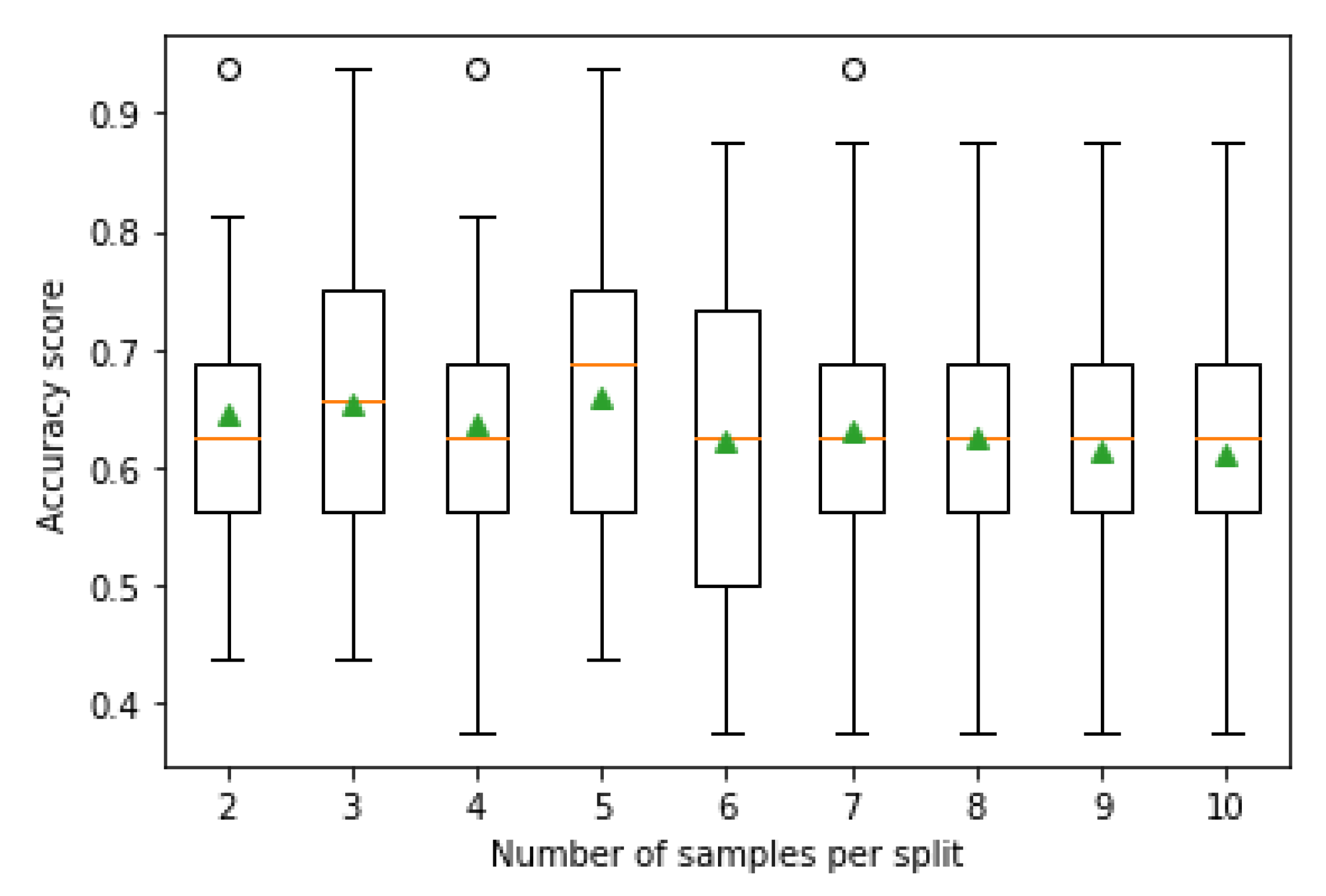
  • Minimum Number of Samples per Split: The last hyperparameter for optimizing is the number of samples in a tree node before any split. The tree adds a new split that occurs when the number of samples divides equally or if the value exceeds. The argument “min_samples_split” represents the minimum number of samples required to split an internal node, and the default value is two samples. Smaller numbers of samples result in more splits and a more rooted, more specialized tree. In turn, this can mean a lower correlation between the predictions made by trees in the ensemble and potentially lift performance.

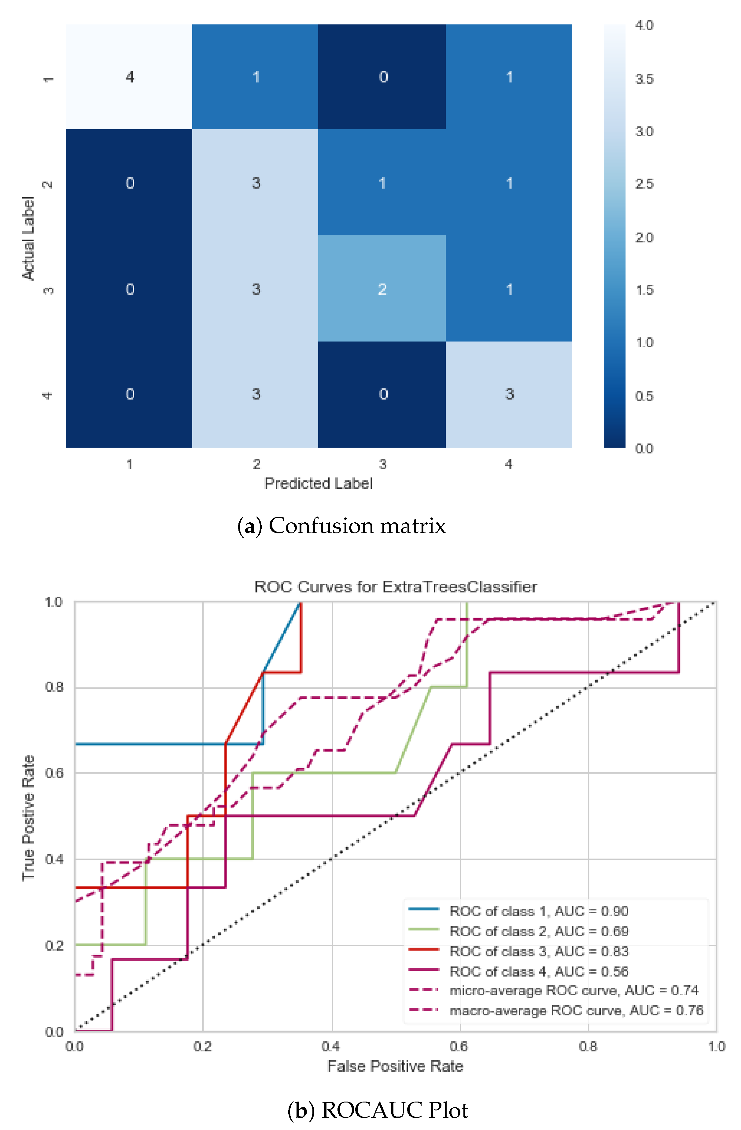
5.5. Results and Analysis

In this section, the results are visualized and analyzed using a box and whisker plot (or boxplot for short) and reference table to list the respective mean accuracy. As an alternative to histograms, boxplots help understand the distribution of sample data. Each dataset is examined using three models created against each hyperparameter tuning factor. Table 4, Table 5, Table 6, Table 7, Table 8, Table 9, Table 10, Table 11, Table 12, Table 13, Table 14 and Table 15 show the mean accuracy of the models are tuning the available hyperparameters, and Figure 15, Figure 16, Figure 17, Figure 18, Figure 19, Figure 20, Figure 21, Figure 22, Figure 23, Figure 24, Figure 25 and Figure 26 show the corresponding distribution of accuracy over the data.
Table 4, Table 5 and Table 6 illustrate the outcomes for Ecuador after tuning the hyperparameters. The total number of features considered in the study is eight. The boxplot is formed to understand the distribution of accuracy observed across the sample data against different input features. The orange line in each box acts as the median for summarizing the sensible data, and the triangle inside the box represents the group means. The vertical line called the whisker represents the sensible distribution of the values. The small circles outside the whisker in a few of the boxplots represent the possible outliers present in the dataset. The outlier is the sample data, unlike the rest of the data, and often does not make sense for the classifier.
In Figure 15, the overall performance of tuning the feature selection is better than configuring the two hyperparameters. In addition, the mean accuracy achieved in this scenario has slight growth compared to the accuracy obtained before optimizing the hyperparameters (64%). The wall area displays a high impact on attaining the required accuracy, although the accuracy differences might or might not be statistically significant. In the boxplot, feature numbers 3 and 5 on the x-axis show peaks, and 7 is low. The boxplot has different feature input data on the x-axis and accuracy scored by each of them on the y-axis. In most cases, the box plot’s median is overlapping the mean score, which means that the distribution is symmetric.
Table 5 illustrates that, as the number of samples per split increases, the accuracy is decreased. In between 5 to 7 number of samples, the predictive accuracy is showing a similar trend. The boxplot in the given Figure 16 has the number of samples per split on the x-axis and accuracy scores for each sample split set on the y-axis. The data distribution is not even, and the values are falling below the 25th percentile. In addition, the mean and median are not overlapping for most cases, and there are few outliers in the case of 3, 4, and 5 number of samples per split.
Results after hyper-tuning the number of trees in an ensemble are shown in Figure 17. Table 6 shows that accuracy increases with the high number of trees; 40 tree ensemble attains 60% accuracy. The boxplot in Figure 17 is skewed left (also called negatively skewed), with 40 trees in one sample; the distribution of the sample data’s value is not uniform as the mean and median are not overlapping.
Figure 18 shows the result of the predictive accuracies achieved after tuning different feature inputs. The Captive Column shows the highest impact on model performance based on the accuracy value. In Table 7, the boxplots are almost symmetric except for the Column Area. There are few visible outliers as well among the input data of the Column Area.
The boxplot result is comparatively asymmetric for tuning the sample per split, and few outliers are present in the input data. Accuracy data on Table 8 present similar results like Ecuador’s performance. A fewer or moderate number of samples per split have better predictive accuracy than the higher samples per split. The boxplots on Figure 19 side are not symmetric, and they are somewhat skewed. The outcome of tuning the feature parameters and the number of samples per split does not significantly change the model’s average score.
Only the number of trees has shown growth in predictive accuracy in Table 9 as compared before and after applying hyperparameter tuning. In addition, 100 is the default hyperparameter value for the number of trees, but, based on the sample size, it may vary from 10 to 5000. The individual box plot and the mean accuracy scores clearly show that the score is lowest when the tree numbers are less, and the score goes high when the number of trees is 30. Further increase in tree number might not be useful in scoring high accuracy as the sample dataset is small. The median of the box plot and the mean accuracy score is not necessarily overlapping except for an ensemble with 40 trees. The predictive accuracy list shows that 20 to 30 trees for creating the ensemble moderately fit the model samples. A similar result is showcased in the boxplots in Figure 20. With 30 trees, the model has shown higher accuracy, and it is skewed left (negatively skewed) according to Figure 20 and Table 9. The whisker line for 20 number of trees is visibly drawn towards the bottom end, which indicates the practical value of the data allocation.
Figure 21, Figure 22 and Figure 23 are the results for accuracy scores generated by models for Nepal after tuning the hyperparameters. Nepal achieved no compelling improvement in accuracy score, compared to what it achieved before optimizing the hyperparameters. One possible reason behind the result could be the high variance of the test harness.
In Table 10, the results after hyper-tuning different feature parameters are presented. The mean accuracy shows that, overall, all the features attain a similar accuracy; total floor area and Captive column are slightly on the higher side. The boxplots on Figure 21 illustrate that most data distribution is between the 25th and 50th percentile. The boxplots are skewed in nature.
Outcome after altering the number of samples per split are illustrated in Figure 22. The mean accuracy presented in Table 11 illustrates that an intermediate number of samples per split give decent result, e.g., 65 to 67% for 4 to 6 sample size per split. As the number of samples per split increases, there is a decline in the accuracy. The boxplots illustrate slight skewness in the data distribution. There are few outliers for a high number of samples per split.
Table 12 presents the result after tuning the number of trees in an ensemble. The scores shown on the right side for the mean accuracy of the model depicts that with a higher number of trees in an ensemble, the model performs better with the unseen examples. The boxplots in Figure 23 have an almost symmetric result and have overlapping means and median. There are very few outliers available in the sample data.
Pohang has got the minimum number of examples in its dataset, reflecting in the outputs. The outcomes after tuning the hyperparameters are not symmetric for most cases. Before configuring the hyperparameters or else tuning the number of trees, the number of samples per split is below the scale.
Before accommodating the hyperparameters, Pohang showed an accuracy of 67%. Only after tuning the features, the accuracy score is high, as it is clear from Table 13. Every input feature has almost achieved similar accuracy in between 70% to 72%. The boxplot results shown in Figure 24 show skewness, which is apparent as almost all the means and median are non-overlapping except for the Masonry wall area (EW); few outliers are also visible in the sample data.
Table 14 shows the mean accuracy results after tuning the number of samples per split. With 2–9 samples, the model performed moderately while the higher value, like 10 number of samples per split, degrades the accuracy. The boxplots shown in Figure 25 have skewness in the distribution, and there are few outliers in the sample input.
Results in Table 15 are for mean accuracy achieved after hyper-tuning the number of trees in an ensemble. The result shows that a moderately higher number of trees make a compelling ensemble and efficient accuracy. The boxplots illustrated in Figure 26 show essentially similar patterns except for the ensemble with ten trees. There are a few outliers present as well with the smallest ensemble.

6. Discussion and Conclusions

The study aimed to investigate ML techniques on RVS and compare each technique’s efficiency for this issue. Therefore, the conclusion can be divided into two parts; one is related to the different ML efficiencies, and the other one is towards the future of RVS with the application of ML.

6.1. Adequacy of ML Techniques

The study utilized various ML algorithms, such as SVM, KNN, Bagging, RF, and ET, for categorizing the RC buildings based on their vulnerability subjected to a seismic event. The input datasets are created from the building samples collected from four real-time earthquakes in Ecuador, Haiti, Nepal, and Pohang. Each dataset is approached by every algorithm utilizing the default parameter values.
Bias and variance are essential factors to understand the performance of the models. Biased models are weak and under fitted. There is a significant disparity between the actual data and the predicted data—whereas, with high variance, the models fit the actual data but can not generalize new data well out of that basis.
In the study, ET performed well with all four datasets compared to the rest of the ML models leaving behind Random Forest. ET and RF ensemble methods have similar tree growing procedures, and both randomly select a feature of the subset while partitioning for each node. However, RF has high variance as the algorithm sub-samples the input data with duplicates. At the same time, ET uses complete original sample data. In addition, RF finds the optimum split while splitting the nodes, but ET goes for random selection. Henceforth, ET is computationally economical and faster than RF, and for high order computational problems, ET would fit better than other supervised learning models.
Furthermore, the ET model for each case study is configured by optimizing the hyperparameters. The results before and after the hyperparameter tuning or optimization have shown slight improvement. RF stood as the second performer among the candidate classifiers. One potential argument behind not achieving substantial growth in the accuracy score after optimizing the hyperparameters for ET might be the quality, size of the datasets, and high variance in the test data. This study’s input datasets are of moderate size and quality because of the lack of proper resources. ET is an ensemble method created by multiple random trees, and its approach is to leverage the power of the crowd (trees) instead of one tree and consider the majority of the voting for the final decision. Thus, ET requires big datasets, which is essential for the model to give an optimized result. For datasets with high variance, adding bias can neutralize it. Furthermore, the study may get extended using big and good quality datasets.

6.2. Applicability of ML-Based Methods to RVS Purposes

The study concludes that the assessed vulnerability classes were very close to the actual damage levels observed in the buildings, which, in comparison to previous methods, provided a more reliable distribution between different damage levels. The proposed method is more accurate than other methods as this rate shows a significant improvement of about 2% to 35% compared to methods stated previously by [5,15,17,18,27]. However, supervised ML techniques are data dependent, and the scope of this study was on RC buildings. The selected parameters for this evaluation are also more comfortable to be measured; moreover, they can be modified based on the availability or demands of experts. Therefore, the application of the proposed method can be adapted for other countries in the world but need to give specific or different types of buildings by providing enough data for training from the selected location. Nevertheless, besides financial benefits and better natural disaster management planning, this achievement also makes building retrofitting more intelligent and saves its residents’ lives. It must be mentioned that it is not expected from RVS methods to have high accuracy and an exact estimate of the possible damage. Since the proposed method is based on MCE, it can be implemented for each studied region and building type. In reality, an overwhelming number of factors and significant parameters play roles in the vulnerability of a building. The main aim of the RVS method is to obtain acceptable classification and initial assessment of damage and be prepared to prevent catastrophe. Benefits such as proper budget allocation and prioritization of building retrofitting and providing measures to prevent buildings and occupants’ damage benefit this method. Moreover, in future studies, more data and parameters such as different structural types, soil conditions, distance to faults, age of buildings, and remote sensing data can be considered.

Author Contributions

Conceptualization, E.H. and V.K.; methodology, E.H. and V.K.; validation, T.L. and E.H.; formal analysis, E.H. and V.K.; investigation, K.J. and V.K.; resources, E.H.; data curation, K.J. and V.K.; writing—original draft preparation, E.H., K.J., V.K., S.R. and R.R.D.; writing—review and editing, E.H., K.J., V.K. and S.R.; visualization, E.H. and V.K.; supervision, E.H. and T.L.; project administration, E.H. and T.L. All authors have read and agreed to the published version of the manuscript.

Funding

This research received no external funding.

Institutional Review Board Statement

Not applicable.

Informed Consent Statement

Not applicable.

Data Availability Statement

Not applicable.

Acknowledgments

We acknowledge the support of the German Research Foundation (DFG) and the Bauhaus-Universität Weimar within the Open-Access Publishing Program. In addition, the ShakeMap and materials are courtesy of the U.S. Geological Survey.

Conflicts of Interest

The authors declare no conflict of interest.

Abbreviations

The following abbreviations are used in this manuscript:
ACIAmerican Concrete Institute
ANNArtificial Neural Network
AUCArea under the Curve
ETExtra Tree
ETEExtra Tree Ensemble
ESPOLEscuela Superior Politécnica del Litoral
FEMAFederal Emergency Management Agency
KNNK-Nearest Neighbor
MCEMaximum Considered Earthquake
MMModified Mercalli
MLMachine Learning
RCReinforced Concrete
RFRandom Forest
ROCReceiver Operating Characteristics
RVSRapid Visual Screening
SVASeismic Vulnerability Assessment
SVMSupport Vector Machine

References

  1. FEMA P-154. Rapid Visual Screening of Buildings for Potential Seismic Hazards: A Handbook, 3rd ed.; Homeland Security Department, Federal Emergency Management Agency: Washington, DC, USA, 2015. [Google Scholar]
  2. Harirchian, E.; Hosseini, S.E.A.; Jadhav, K.; Kumari, V.; Rasulzade, S.; Işık, E.; Wasif, M.; Lahmer, T. A review on application of soft computing techniques for the rapid visual safety evaluation and damage classification of existing buildings. J. Build. Eng. 2021, 43, 102536. [Google Scholar] [CrossRef]
  3. Yadollahi, M.; Adnan, A.; Mohamad zin, R. Seismic Vulnerability Functional Method for Rapid Visual Screening of Existing Buildings. Arch. Civ. Eng. 2012, 3, 363–377. [Google Scholar] [CrossRef] [Green Version]
  4. Yang, Y.; Goettel, K.A. Enhanced Rapid Visual Screening (E-RVS) Method for Prioritization of Seismic Retrofits in Oregon; Oregon Department of Geology and Mineral Industries: Portland, OR, USA, 2007. [Google Scholar]
  5. Harirchian, E.; Jadhav, K.; Mohammad, K.; Aghakouchaki Hosseini, S.E.; Lahmer, T. A comparative study of MCDM methods integrated with rapid visual seismic vulnerability assessment of existing RC structures. Appl. Sci. 2020, 10, 6411. [Google Scholar] [CrossRef]
  6. Jain, S.; Mitra, K.; Kumar, M.; Shah, M. A proposed rapid visual screening procedure for seismic evaluation of RC-frame buildings in India. Earthq. Spectra 2010, 26, 709–729. [Google Scholar] [CrossRef]
  7. Chanu, N.; Nanda, R. A Proposed Rapid Visual Screening Procedure for Developing Countries. Int. J. Geotech. Earthq. Eng. 2018, 9, 38–45. [Google Scholar] [CrossRef]
  8. Sinha, R.; Goyal, A. A National Policy for Seismic Vulnerability Assessment of Buildings and Procedure for Rapid Visual Screening of Buildings for Potential Seismic Vulnerability; Report to Disaster Management Division; Ministry of Home Affairs, Government of India: Mumbai, India, 2004. [Google Scholar]
  9. Rai, D.C. Review of Documents on Seismic Evaluation of Existing Buildings; IIT Kanpur and Gujarat State Disaster Mitigation Authority: Gandhinagar, India, 2005; pp. 1–120. [Google Scholar]
  10. Mishra, S. Guide Book for Integrated Rapid Visual Screening of Buildings for Seismic Hazard; TARU Leading Edge Private Ltd.: New Delhi, India, 2014. [Google Scholar]
  11. Luca, F.; Verderame, G. Seismic Vulnerability Assessment: Reinforced Concrete Structures; Springer: Berlin/Heidelberg, Germany, 2014. [Google Scholar]
  12. Chanu, N.; Nanda, R. Rapid Visual Screening Procedure of Existing Building Based on Statistical Analysis. Int. J. Disaster Risk Reduct. 2018, 28, 720–730. [Google Scholar]
  13. Özhendekci, N.; Özhendekci, D. Rapid Seismic Vulnerability Assessment of Low- to Mid-Rise Reinforced Concrete Buildings Using Bingöl’s Regional Data. Earthq. Spectra 2012, 28, 1165–1187. [Google Scholar] [CrossRef]
  14. Harirchian, E.; Lahmer, T. Improved Rapid Assessment of Earthquake Hazard Safety of Structures via Artificial Neural Networks. In Proceedings of the 2020 5th International Conference on Civil Engineering and Materials Science (ICCEMS 2020), Singapore, 15–18 May 2020; IOP Publishing: Bristol, UK, 2020; Volume 897, p. 012014. [Google Scholar]
  15. Harirchian, E.; Lahmer, T.; Rasulzade, S. Earthquake Hazard Safety Assessment of Existing Buildings Using Optimized Multi-Layer Perceptron Neural Network. Energies 2020, 13, 2060. [Google Scholar] [CrossRef] [Green Version]
  16. Arslan, M.; Ceylan, M.; Koyuncu, T. An ANN approaches on estimating earthquake performances of existing RC buildings. Neural Netw. World 2012, 22, 443–458. [Google Scholar] [CrossRef] [Green Version]
  17. Roeslin, S.; Ma, Q.; Juárez-Garcia, H.; Gómez-Bernal, A.; Wicker, J.; Wotherspoon, L. A machine learning damage prediction model for the 2017 Puebla-Morelos, Mexico, earthquake. Earthq. Spectra 2020, 36, 314–339. [Google Scholar] [CrossRef]
  18. Mangalathu, S.; Sun, H.; Nweke, C.C.; Yi, Z.; Burton, H.V. Classifying earthquake damage to buildings using machine learning. Earthq. Spectra 2020, 36, 183–208. [Google Scholar] [CrossRef]
  19. Tesfamariam, S.; Liu, Z. Earthquake induced damage classification for reinforced concrete buildings. Struct. Saf. 2010, 32, 154–164. [Google Scholar] [CrossRef]
  20. Harirchian, E.; Kumari, V.; Jadhav, K.; Raj Das, R.; Rasulzade, S.; Lahmer, T. A machine learning framework for assessing seismic hazard safety of reinforced concrete buildings. Appl. Sci. 2020, 10, 7153. [Google Scholar] [CrossRef]
  21. Harirchian, E.; Harirchian, A. Earthquake Hazard Safety Assessment of Buildings via Smartphone App: An Introduction to the Prototype Features-30. In 30. Forum Bauinformatik: Von jungen Forschenden für junge Forschende: September 2018, Informatik im Bauwesen; Professur Informatik im Bauwesen, Bauhaus-Universität Weimar: Weimar, Germany, 2018; pp. 289–297. [Google Scholar]
  22. Yu, Q.; Wang, C.; McKenna, F.; Stella, X.Y.; Taciroglu, E.; Cetiner, B.; Law, K.H. Rapid visual screening of soft-story buildings from street view images using deep learning classification. Earthq. Eng. Eng. Vib. 2020, 19, 827–838. [Google Scholar] [CrossRef]
  23. Ketsap, A.; Hansapinyo, C.; Kronprasert, N.; Limkatanyu, S. Uncertainty and fuzzy decisions in earthquake risk evaluation of buildings. Eng. J. 2019, 23, 89–105. [Google Scholar] [CrossRef]
  24. Mandas, A.; Dritsos, S. Vulnerability assessment of RC structures using fuzzy logic. WIT Trans. Ecol. Environ. 2004, 77, 10. [Google Scholar]
  25. Tesfamariam, S.; Saatcioglu, M. Seismic vulnerability assessment of reinforced concrete buildings using hierarchical fuzzy rule base modeling. Earthq. Spectra 2010, 26, 235–256. [Google Scholar] [CrossRef]
  26. Şen, Z. Rapid visual earthquake hazard evaluation of existing buildings by fuzzy logic modeling. Expert Syst. Appl. 2010, 37, 5653–5660. [Google Scholar] [CrossRef]
  27. Harirchian, E.; Lahmer, T. Developing a hierarchical type-2 fuzzy logic model to improve rapid evaluation of earthquake hazard safety of existing buildings. In Structures; Elsevier: Edinburgh, UK, 2020; Volume 28, pp. 1384–1399. [Google Scholar]
  28. Harirchian, E.; Lahmer, T. Improved Rapid Visual Earthquake Hazard Safety Evaluation of Existing Buildings Using a Type-2 Fuzzy Logic Model. Appl. Sci. 2020, 10, 2375. [Google Scholar] [CrossRef] [Green Version]
  29. Sucuoglu, H.; Yazgan, U.; Yakut, A. A Screening Procedure for Seismic Risk Assessment in Urban Building Stocks. Earthq. Spectra 2007, 23, 441–458. [Google Scholar] [CrossRef]
  30. Morfidis, K.; Kostinakis, K. Seismic parameters’ combinations for the optimum prediction of the damage state of R/C buildings using neural networks. Adv. Eng. Softw. 2017, 106, 1–16. [Google Scholar] [CrossRef]
  31. Jain, S.; Mitra, K.; Kumar, M.; Shah, M. A Rapid Visual Seismic Assessment Procedure for RC Frame Buildings in India. In Proceedings of the 9th US National and 10th Canadian Conference on Earthquake Engineering, Toronto, ON, Canada, 29 July 2010. [Google Scholar]
  32. Aldemir, A.; Sahmaran, M. Rapid screening method for the determination of seismic vulnerability assessment of RC building stocks. Bull. Earthq. Eng. 2019, 18, 1401–1416. [Google Scholar]
  33. Askan, A.; Yucemen, M. Probabilistic methods for the estimation of potential seismic damage: Application to reinforced concrete buildings in Turkey. Struct. Saf. 2010, 32, 262–271. [Google Scholar] [CrossRef]
  34. Morfidis, K.; Kostinakis, K. Use of Artificial Neural Networks in the r/c Buildings’ Seismic Vulnerabilty Assessment: The Practical Point of View. In Proceedings of the 7th International Conference on Computational Methods in Structural Dynamics and Earthquake Engineering, Crete, Greece, 24–26 June 2019. [Google Scholar]
  35. Dritsos, S.; Moseley, V. A Fuzzy Logic Rapid Visual Screening Procedure to Identify Buildings at Seismic Risk; Beton-Und Stahlbetonbau: Ernst & Sohn Verlag für Architektur und Technische Wissenschaften GmbH & Co. KG: Berlin, Germany, 2013; pp. 136–143. Available online: https://www.researchgate.net/publication/295594396_A_fuzzy_logic_rapid_visual_screening_procedure_to_identify_buildings_at_seismic_risk (accessed on 30 June 2020).
  36. Sun, H.; Burton, H.V.; Huang, H. Machine learning applications for building structural design and performance assessment: State-of-the-art review. J. Build. Eng. 2020, 33, 101816. [Google Scholar] [CrossRef]
  37. Harirchian, E.; Lahmer, T.; Kumari, V.; Jadhav, K. Application of Support Vector Machine Modeling for the Rapid Seismic Hazard Safety Evaluation of Existing Buildings. Energies 2020, 13, 3340. [Google Scholar] [CrossRef]
  38. Zhang, Z.; Hsu, T.Y.; Wei, H.H.; Chen, J.H. Development of a Data-Mining Technique for Regional-Scale Evaluation of Building Seismic Vulnerability. Appl. Sci. 2019, 9, 1502. [Google Scholar] [CrossRef] [Green Version]
  39. Christine, C.A.; Chandima, H.; Santiago, P.; Lucas, L.; Chungwook, S.; Aishwarya, P.; Andres, B. A cyberplatform for sharing scientific research data at DataCenterHub. Comput. Sci. Eng. 2018, 20, 49. [Google Scholar]
  40. Sim, C.; Laughery, L.; Chiou, T.C.; Weng, P.W. 2017 Pohang Earthquake—Reinforced Concrete Building Damage Survey DEEDS; Purdue University Research Repository: Lafayette, IN, USA, 2018; Available online: https://datacenterhub.org/resources/14728 (accessed on 2 June 2020).
  41. Sim, C.; Villalobos, E.; Smith, J.P.; Rojas, P.; Pujol, S.; Puranam, A.Y.; Laughery, L.A. Performance of Low-Rise Reinforced Concrete Buildings in the 2016 Ecuador Earthquake, Purdue University Research Repository, United States. 2017. Available online: https://purr.purdue.edu/publications/2727/1 (accessed on 10 June 2020).
  42. NEES: The Haiti Earthquake Database; DEEDS, Purdue University Research Repository: Lafayette, IN, USA, 2017; Available online: https://datacenterhub.org/resources/263 (accessed on 2 June 2020).
  43. Shah, P.; Pujol, S.; Puranam, A.; Laughery, L. Database on Performance of Low-Rise Reinforced Concrete Buildings in the 2015 Nepal Earthquake; DEEDS, Purdue University Research Repository: Lafayette, IN, USA, 2015; Available online: https://datacenterhub.org/resources/238 (accessed on 10 June 2020).
  44. Toulkeridis, T.; Chunga, K.; Rentería, W.; Rodriguez, F.; Mato, F.; Nikolaou, S.; D’Howitt, M.C.; Besenzon, D.; Ruiz, H.; Parra, H.; et al. THE 7.8 M w EARTHQUAKE AND TSUNAMI OF 16 th April 2016 IN ECUADOR: Seismic Evaluation, Geological Field Survey and Economic Implications. Sci. Tsunami Hazards 2017, 36, 78–123. [Google Scholar]
  45. Vera-Grunauer, X. Geer-Atc Mw7.8 Ecuador 4/16/16 Earthquake Reconnaissance Part II: Selected Geotechnical Observations. In Proceedings of the 16th World Conference on Earthquake Engineering (WCEE), Santiago, Chile, 9–13 January 2017. [Google Scholar]
  46. O’Brien, P.; O’Brien, P.; Eberhard, M.; Haraldsson, O.; Irfanoglu, A.; Lattanzi, D.; Lauer, S.; Pujol, S. Measures of the Seismic Vulnerability of Reinforced Concrete Buildings in Haiti. Earthq. Spectra 2011, 27, S373–S386. [Google Scholar] [CrossRef]
  47. De León, R.O. Flexible soils amplified the damage in the 2010 Haiti earthquake. Earthq. Resist. Eng. Struct. IX 2013, 132, 433–444. [Google Scholar]
  48. U.S. Geological Survey (USGS) 2010; U.S. Geological Survey: Reston, VA, USA, 2010.
  49. Collins, B.D.; Jibson, R.W. Assessment of Existing and Potential Landslide Hazards Resulting from the April 25, 2015 Gorkha, Nepal Earthquake Sequence; Ver. 1.1, August 2015; U.S. Geological Survey Open-File Report 2015–1142; U.S. Geological Survey: Reston, VA, USA, 2015; 50p. [Google Scholar] [CrossRef] [Green Version]
  50. Tallett-Williams, S.; Gosh, B.; Wilkinson, S.; Fenton, C.; Burton, P.; Whitworth, M.; Datla, S.; Franco, G.; Trieu, A.; Dejong, M.; et al. Site amplification in the Kathmandu Valley during the 2015 M7. 6 Gorkha, Nepal earthquake. Bull. Earthq. Eng. 2016, 14, 3301–3315. [Google Scholar] [CrossRef]
  51. Işık, E.; Büyüksaraç, A.; Ekinci, Y.L.; Aydın, M.C.; Harirchian, E. The Effect of Site-Specific Design Spectrum on Earthquake-Building Parameters: A Case Study from the Marmara Region (NW Turkey). Appl. Sci. 2020, 10, 7247. [Google Scholar] [CrossRef]
  52. Grigoli, F.; Cesca, S.; Rinaldi, A.P.; Manconi, A.; Lopez-Comino, J.A.; Clinton, J.; Westaway, R.; Cauzzi, C.; Dahm, T.; Wiemer, S. The November 2017 Mw 5.5 Pohang earthquake: A possible case of induced seismicity in South Korea. Science 2018, 360, 1003–1006. [Google Scholar] [CrossRef] [PubMed] [Green Version]
  53. Kim, H.S.; Sun, C.G.; Cho, H.I. Geospatial assessment of the post-earthquake hazard of the 2017 Pohang earthquake considering seismic site effects. ISPRS Int. J. Geo-Inf. 2018, 7, 375. [Google Scholar] [CrossRef] [Green Version]
  54. Ademović, N.; Šipoš, T.K.; Hadzima-Nyarko, M. Rapid assessment of earthquake risk for Bosnia and Herzegovina. Bull. Earthq. Eng. 2020, 18, 1835–1863. [Google Scholar] [CrossRef]
  55. USGS. Earthquake Hazards Program, ShakeMap. Available online: https://earthquake.usgs.gov/data/shakemap (accessed on 2 May 2021).
  56. USGS. Earthquake Hazards Program, ShakeMap of Ecuador Earthquake 2016. Available online: https://earthquake.usgs.gov/earthquakes/eventpage/us20005j32/shakemap/intensity (accessed on 10 May 2021).
  57. USGS. Earthquake Hazards Program, ShakeMap of Haiti Earthquake 2010. Available online: https://earthquake.usgs.gov/earthquakes/eventpage/usp000h60h/shakemap/intensity (accessed on 16 May 2021).
  58. USGS. Earthquake Hazards Program, ShakeMap of Nepal Earthquake 2015. Available online: ttps://earthquake.usgs.gov/earthquakes/eventpage/us20002ejl/shakemap/intensity (accessed on 12 June 2021).
  59. USGS. Earthquake Hazards Program, ShakeMap of Pohang Earthquake 2017. Available online: https://earthquake.usgs.gov/earthquakes/eventpage/us2000bnrs/shakemap/intensity (accessed on 13 June 2021).
  60. Stone, H. Exposure and Vulnerability for Seismic Risk Evaluations. Ph.D. Thesis, UCL (University College London), London, UK, 2018. [Google Scholar]
  61. Harirchian, E.; Lahmer, T. Earthquake Hazard Safety Assessment of Buildings via Smartphone App: A Comparative Study. IOP Conf. Ser. Mater. Sci. Eng. 2019, 652, 012069. [Google Scholar] [CrossRef]
  62. Harirchian, E.; Jadhav, K.; Kumari, V.; Lahmer, T. ML-EHSAPP: A prototype for machine learning-based earthquake hazard safety assessment of structures by using a smartphone app. Eur. J. Environ. Civ. Eng. 2021, 25, 1–21. [Google Scholar] [CrossRef]
  63. Yakut, A.; Aydogan, V.; Ozcebe, G.; Yucemen, M. Preliminary Seismic Vulnerability Assessment of Existing Reinforced Concrete Buildings in Turkey. In Seismic Assessment and Rehabilitation of Existing Buildings; Springer: Dordrecht, The Netherlands, 2003; pp. 43–58. [Google Scholar]
  64. Hassan, A.F.; Sozen, M.A. Seismic vulnerability assessment of low-rise buildings in regions with infrequent earthquakes. ACI Struct. J. 1997, 94, 31–39. [Google Scholar]
  65. Caruana, R.; Niculescu-Mizil, A. An empirical comparison of supervised learning algorithms. In Proceedings of the 23rd International Conference on Machine Learning, Pittsburgh, PA, USA, 25–29 June 2006; pp. 161–168. [Google Scholar] [CrossRef] [Green Version]
  66. Géron, A. Hands-on Machine Learning with Scikit-Learn and TensorFlow: Concepts, Tools, and Techniques to Build Intelligent Systems O’Reilly Media; O’Reilly: Sebastopol, CA, USA, 2017. [Google Scholar]
  67. Vapnik, V.N.; Golowich, S.E. Support Vector Method for Function Estimation. U.S. Patent 6,269,323, 31 July 2001. [Google Scholar]
  68. Fix, E. Discriminatory Analysis. Nonparametric Discrimination: Consistency Properties. Int. Stat. Rev./Rev. Int. Stat. 1989, 57, 238–247. [Google Scholar] [CrossRef]
  69. Cover, T.; Hart, P. Nearest neighbor pattern classification. IEEE Trans. Inf. Theory 1967, 13, 21–27. [Google Scholar] [CrossRef]
  70. Breiman, L. Bagging predictors. Mach. Learn. 1996, 24, 123–140. [Google Scholar] [CrossRef] [Green Version]
  71. Geurts, P.; Ernst, D.; Wehenkel, L. Extremely randomized trees. Mach. Learn. 2006, 63, 3–42. [Google Scholar] [CrossRef] [Green Version]
  72. Breiman, L. Random forests. Mach. Learn. 2001, 45, 5–32. [Google Scholar] [CrossRef] [Green Version]
  73. Ho, T. Random decision forests. In Proceedings of the Third International Conference on Document Analysis and Recognition, ICDAR 1995, Montreal, QC, Canada, 14–16 August 1995; Volume 1, pp. 278–282. [Google Scholar]
  74. Ho, T.K. The random subspace method for constructing decision forests. IEEE Trans. Pattern Anal. Mach. Intell. 1998, 20, 832–844. [Google Scholar]
  75. Amit, Y.; Geman, D. Shape quantization and recognition with randomized trees. Neural Comput. 1997, 9, 1545–1588. [Google Scholar] [CrossRef] [Green Version]
  76. Fawagreh, K.; Gaber, M.M.; Elyan, E. Random forests: From early developments to recent advancements. Syst. Sci. Control Eng. Open Access J. 2014, 2, 602–609. [Google Scholar] [CrossRef] [Green Version]
  77. Webb, G.I. Multiboosting: A technique for combining boosting and wagging. Mach. Learn. 2000, 40, 159–196. [Google Scholar] [CrossRef] [Green Version]
  78. Breiman, L. Randomizing outputs to increase prediction accuracy. Mach. Learn. 2000, 40, 229–242. [Google Scholar] [CrossRef] [Green Version]
  79. Liaw, A.; Wiener, M. Classification and regression by randomForest. R News 2002, 2, 18–22. [Google Scholar]
  80. Chawla, N.V.; Bowyer, K.W.; Hall, L.O.; Kegelmeyer, W.P. SMOTE: Synthetic minority over-sampling technique. J. Artif. Intell. Res. 2002, 16, 321–357. [Google Scholar] [CrossRef]
  81. May, R.J.; Maier, H.R.; Dandy, G.C. Data splitting for artificial neural networks using SOM-based stratified sampling. Neural Netw. 2010, 23, 283–294. [Google Scholar] [CrossRef] [PubMed]
  82. Lewis, H.; Brown, M. A generalized confusion matrix for assessing area estimates from remotely sensed data. Int. J. Remote Sens. 2001, 22, 3223–3235. [Google Scholar] [CrossRef]
  83. Sun, Y.; Gong, H.; Li, Y.; Zhang, D. Hyperparameter Importance Analysis based on N-RReliefF Algorithm. Int. J. Comput. Commun. Control 2019, 14, 557–573. [Google Scholar] [CrossRef] [Green Version]
Figure 1. ShakeMap and intensity scale for the (a) Ecuador; (b) Haiti; (c) Nepal; and (d) Pohang Earthquake [55,56,57,58,59].
Applsci 11 07540 g001
Figure 2. Properties of selected earthquakes.
Applsci 11 07540 g002
Figure 3. Distribution of input data based on the damage scale: Data from Ecuador and Haiti have a distribution over three categories, whereas the data for Nepal and Pohang are classified with four different grades.
Applsci 11 07540 g003
Figure 4. The histogram plot shows the distribution of data of (a) Captive Columns, (b) Column Area, (e) Masonry Wall Area (EW), (f) Masonry Wall Area (NS), (g) No. of Floor, and (h) Total Floor Area for Ecuador.
Applsci 11 07540 g004
Figure 5. Distribution of data of (a) Captive Columns, (b) Column Area, (e) Masonry Wall Area (EW), (f) Masonry Wall Area (NS), (g) No. of Floor, and (h) Total Floor Area for Haiti.
Applsci 11 07540 g005
Figure 6. The histogram plot shows the distribution of data of (a) Captive Columns, (b) Column Area, (e) Masonry Wall Area (EW), (f) Masonry Wall Area (NS), (g) No. of Floor, and h) Total Floor Area for Nepal.
Applsci 11 07540 g006
Figure 7. Data distribution of (a) Captive Columns, (b) Column Area, (c) Concrete Wall Area (EW), (d) Concrete Wall Area (NS), (g) No. of Floor, and (h) Total Floor Area for Pohang.
Applsci 11 07540 g007
Figure 8. Methodology Flowchart: The given flowchart shows the steps involved to build and evaluate different classifiers on the given input dataset.
Applsci 11 07540 g008
Figure 9. The chart involves the predictive accuracy acquired by each candidate classifier against every dataset.
Applsci 11 07540 g009
Figure 10. Structure of a confusion matrix for a binary classification.
Applsci 11 07540 g010
Figure 11. Performance of ET on Ecuador.
Applsci 11 07540 g011
Figure 12. Performance of ET on Haiti.
Applsci 11 07540 g012aApplsci 11 07540 g012b
Figure 13. Performance of ET on Nepal.
Applsci 11 07540 g013
Figure 14. Performance of ET on Pohang.
Applsci 11 07540 g014
Figure 15. Ecuador: Boxplot to represent the mean accuracy distribution achieved by hyper-tuning the input features.
Applsci 11 07540 g015
Figure 16. Ecuador: Boxplot to illustrate the mean accuracy distribution by hyper-tuning the minimum number of samples per split.
Applsci 11 07540 g016
Figure 17. Ecuador: Boxplot to represent the mean accuracy distribution achieved by tuning number of trees for every ensemble.
Applsci 11 07540 g017
Figure 18. Haiti: Boxplot to represent the mean accuracy distribution achieved by hyper-tuning the input features.
Applsci 11 07540 g018
Figure 19. Haiti: Boxplot to illustrate the mean accuracy distribution by hyper-tuning the minimum number of samples per split.
Applsci 11 07540 g019
Figure 20. Haiti: Boxplot represents the mean accuracy distribution achieved by tuning the number of trees for every ensemble.
Applsci 11 07540 g020
Figure 21. Nepal: Boxplot to represent the mean accuracy distribution achieved by hyper-tuning the input features.
Applsci 11 07540 g021
Figure 22. Nepal: Boxplot to illustrate the mean accuracy distribution by hyper-tuning the minimum number of samples per split.
Applsci 11 07540 g022
Figure 23. Nepal: Boxplot represents the mean accuracy distribution achieved by tuning the number of trees for every ensemble.
Applsci 11 07540 g023
Figure 24. Pohang: Boxplot to represent the mean accuracy distribution achieved by hyper-tuning the input features.
Applsci 11 07540 g024
Figure 25. Pohang: Boxplot to illustrate the mean accuracy distribution by hyper-tuning the minimum number of samples per split.
Applsci 11 07540 g025
Figure 26. Pohang: Boxplot represents the mean accuracy distribution achieved by tuning the number of trees for every ensemble.
Applsci 11 07540 g026
Table 1. Parameters for earthquake hazard safety assessment (adopted from [14,20]).
VariableParameterUnitType
i 1 No. of storyN (1, 2, …)Quantitative
i 2 Total Floor Aream 2 Quantitative
i 3 Column Aream 2 Quantitative
i 4 Concrete Wall Area (Y)m 2 Quantitative
i 5 Concrete Wall Area (X)m 2 Quantitative
i 6 Masonry Wall Area (Y)m 2 Quantitative
i 7 Masonry Wall Area (X)m 2 Quantitative
i 8 Captive ColumnsN (exist = yes = 1, absent = no = 0)Dummy
Table 2. Number of buildings for each earthquake’s dataset.
EarthquakeNo. of Buildings
Ecuador172
Haiti145
Nepal135
Pohang74
Table 3. Damage scale for selected earthquakes (adopted from [40,43]).
Damage ScaleAssociated Risk
1Light: Hairline inclined and flexural cracks were observed in structural elements.
2Moderate: Wider cracks or spalling of concrete was observed.
3Severe: At least one element had a structural failure.
4Collapse: At least one floor slab or part of it lost its elevation.
Table 4. Ecuador: Predictive accuracy score against each input feature.
FeatureMean Accuracy (%)
No. of floor64
Total floor area65
Column area65
Concrete wall area (NS)66
Concrete wall area (EW)67
Masonry wall area (NS)66
Masonry wall area (EW)65
Captive Columns66
Table 5. Ecuador:Predictive accuracy score against number of samples per split.
No. of Sample per SplitMean Accuracy (%)
264
365
465
565
665
765
864
963
1062
Table 6. Ecuador: Predictive accuracy score against number of trees for each ensemble.
Feature (No. of Tree)Mean Accuracy (%)
1063
2064
3065
4068
Table 7. Haiti: Predictive accuracy score against each input feature.
FeatureMean Accuracy (%)
No. of floor61
Total floor area60
Column area62
Concrete wall area (NS)64
Concrete wall area (EW)63
Masonry wall area (NS)63
Masonry wall area (EW)63
Captive Columns66
Table 8. Haiti: Predictive accuracy score against number of samples per split.
No. of Sample per SplitMean Accuracy (%)
264
365
464
566
662
763
862
961
1062
Table 9. Haiti: Predictive accuracy score against number of trees for each ensemble.
Feature (No. of Tree)Mean Accuracy (%)
1060
2065
3066
4063
Table 10. Nepal: Predictive accuracy score against each input feature.
FeatureMean Accuracy (%)
No. of floor68
Total floor area70
Column area69
Concrete wall area (NS)68
Concrete wall area (EW)68
Masonry wall area (NS)69
Masonry wall area (EW)68
Captive Columns70
Table 11. Nepal: Predictive accuracy score against number of samples per split.
No. of Sample per SplitMean Accuracy (%)
265
364
467
565
665
764
864
963
1063
Table 12. Nepal: Predictive accuracy score against number of trees for each ensemble.
Feature (No. of Trees)Mean Accuracy (%)
1066
2067
3068
4071
Table 13. Pohang: Predictive accuracy score against each input feature.
FeatureMean Accuracy (%)
No. of floor72
Total floor area70
Column area71
Concrete wall area (NS)70
Concrete wall area (EW)72
Masonry wall area (NS)71
Masonry wall area (EW)71
Captive Columns71
Table 14. Pohang: Predictive accuracy score against the number of samples per split.
No. of Sample per SplitMean Accuracy (%)
262
361
460
560
660
761
860
961
1053
Table 15. Pohang: Predictive accuracy score against number of trees for each ensemble.
No. of TreeMean Accuracy (%)
1061
2063
3065
4064
Publisher’s Note: MDPI stays neutral with regard to jurisdictional claims in published maps and institutional affiliations.

