Article

A CNN Regression Approach to Mobile Robot Localization Using Omnidirectional Images

Department of Systems Engineering and Automation, Miguel Hernández University, 03202 Elche, Spain
*
Author to whom correspondence should be addressed.
Appl. Sci. 2021, 11(16), 7521; https://doi.org/10.3390/app11167521
Submission received: 14 July 2021 / Revised: 10 August 2021 / Accepted: 13 August 2021 / Published: 16 August 2021
(This article belongs to the Special Issue Application of Computer Science in Mobile Robots)

Abstract

:
Understanding the environment is an essential ability for robots to be autonomous. In this sense, Convolutional Neural Networks (CNNs) can provide holistic descriptors of a scene. These descriptors have proved to be robust in dynamic environments. The aim of this paper is to perform hierarchical localization of a mobile robot in an indoor environment by means of a CNN. Omnidirectional images are used as the input of the CNN. Experiments include a classification study in which the CNN is trained so that the robot is able to find out the room where it is located. Additionally, a transfer learning technique transforms the original CNN into a regression CNN which is able to estimate the coordinates of the position of the robot in a specific room. Regarding classification, the room retrieval task is performed with considerable success. As for the regression stage, when it is performed along with an approach based on splitting rooms, it also provides relatively accurate results.

1. Introduction

Localization is an essential ability for a mobile robot to be autonomous. In order to tackle high level tasks, a mobile robot must be able to create a map of the environment, localize itself in this map and perform a path planing strategy in this environment.
To explore the environment the robot must be provided with a sensor system that captures information around it. There exists extensive research related to sensors used with mobile robots, such as SONAR, laser, GPS or cameras [1,2,3,4]. Among them, vision systems have significantly attracted the attention of the scientific community [5,6,7]. Compared to other kinds of systems, cameras are relatively cheap devices and they are capable of extracting a high amount of information from the environment. This work is based on the use of omnidirectional cameras due to their wide field of view since them provide in one single image, 360° information around the robot.
These sensors along with others already mentioned such as SONAR or lasers can provide a precise, robust and economic solution to localization when combined with current Artificial Intelligence (AI)-based visual recognition technologies [8,9], which constitute another growing sector.
The efficiency of omnidirectional images in mapping and localization tasks depends basically on how the visual information is described. Many description methods have been used in mapping tasks carried out by mobile robots [10,11]. Some of these methods extract characteristic points of the environment and an associated descriptor containing certain information that provides invariance to many changes such as lighting, point of view and other transformations. Some of the most used methods are descriptors based on local features such as the scale-invariant feature transform (SIFT) [12], which extracts and describes characteristic points invariant to rotation, scale and change of lighting conditions. Speeded up robust features (SURFs) [13] is based on SIFT points but with more robustness to translation changes and less computational cost.
Other methods are based on global descriptors [14]. The descriptor encodes the information of the whole image instead of only local information. This is the case of Principal Components Analysis (PCA) [15] and methods based on Deep Learning techniques [16,17].
Deep learning is a branch of the artificial intelligence (AI) that in recent years has experienced great improvements due to its potential and hardware development. Deep learning includes tools such as Convolutional Neural Networks (CNNs) that, despite their often computationally expensive training process, have shown excellent results in image classification tasks and recognition [9,16,17,18]. These algorithms allow applying filters in order to extract global descriptors of the input image.
Broadly speaking, the architecture of a CNN consists of an input layer, hidden layers and an output. However, different CNNs architectures can be found in the literature according to the number and typology of the hidden layers and the way they are connected. The selection of the most suitable CNN architecture depends on the task to be performed. For example, some of them such as GoogleNet, ResNetm, VGG or AlexNet are remarkable according to their excellent results in classification [14,19,20,21].
Omnidirectional images in visual navigation are in widespread use [22,23,24,25]. For example, Tanaka et al. [22] propose the use of omnidirectional images to find a solution for the localization of a mobile robot. In particular, they use the panorama obtained from the captured image and perform a correlation method that is then refined using a Kalman filter by incorporating the dynamic information of the robot model. Furthermore, Huei-Yung and Chien-Hsing [23] present a technique for localization of mobile robots based on image feature matching from omnidirectional vision. They estimate the camera motion trajectory based on the catadioptric projection model and create a parallel virtual space simulating the environment in the real world. Compared to these previous works, which use handcrafted features to describe the scenes, our paper presents a different approach. The main contribution of the present paper is a solution to the localization of a mobile robot using deep learning techniques. In this work, two different kinds of CNNs are trained. First, a CNN is trained for classification in order to solve a coarse localization, i.e., to obtain the room or area where the robot is located. Second, for each room or area, a regression CNN is trained to perform a fine localization. Each of these regression CNNs estimates the position of the robot in a specific room or area (X and Y coordinates). Finally, a splitting method for improving the localization in large areas is proposed. This method leads to more precise results in larger areas.
The remainder of the paper is structured as follows. Section 2 presents state of art of CNNs in feature extraction and localization. Then, Section 3 describes the training process we propose training the CNNs with a twofold purpose, to solve the hierarchical localization problem: (a) detection of the room or area where the robot is and (b) estimation of the coordinates of the position of the robot in the previously retrieved zone. Section 4 presents the dataset used in our experiments, which is specially intended for testing localization algorithms under real operation conditions. Then, Section 5 shows the experiments performed related to the classification stage as well as fine localization. Some improvements to enhance the localization results are also displayed. Finally, conclusions and future works are presented in Section 6.

2. Convolutional Neural Networks

Convolutional Neural Networks (CNNs) emerged in 1989 showing great potential in computer vision tasks [26]. Since then, a large number of innovations have made it possible to adapt these networks to challenging current problems with more complex input data.

2.1. Feature Extraction Using CNNs

AlexNet architecture was presented in 2012 [18] and was a great milestone in the area [19], since until then the use of CNNs was limited basically to the recognition of written digits due, mostly, to the hardware limitations of that time. AlexNet is considered by some authors as the first deep convolutional net [9]. This net increased the depth from 5 layers (LeNet [27]) to 8, thus allowing to extend itself to more categories. The more depth a network presents, the better the capacity to adapt to a large number of categories. In addition, the ReLu activation function was employed, which eliminated the gradient fading problem. All this contributed to the network showing excellent results in the ImageNet database ranking. This successful performance was mainly due to the depth of the network, which, despite the high computation time, could be trained and utilized thanks to the use of GPUs in parallel. After that, the ResNet architecture introduced the tendency to skip connections between layers [28] and VGG presented a great performance with the extraction of characteristics at low resolution [29]. Nowadays, there are many different architectures and the quality of their performances depends on the specific application and the variety of training data. A common tendency is to merge different architectures to compensate for deficiencies of one net with the benefits of the other as in the example of Inception-Resnet (Inception v4) [30]. The improvements and innovations in the architectures together with their great potential have favored their presence in many technologies such as robotics. In fact, CNNs have become one of the most popular methods to extract information from images in supervised learning vision applications. For example, da Silva et al. [31] use a CNN to obtain descriptors from omnidirectional images as an approach to solve the localization and navigation problem for mobile robots.
CNNs are trained using a multitude of different images and therefore they have shown robustness to changes in rotation, translation, scale and deformation in images [32,33]. It is worth noting that, regardless the final task for which the CNNs are designed, intermediate layers extract relevant information, i.e., the information in each of these layers can be considered as a global-appearance descriptor of the input image. This means that these descriptors can be used for other tasks or even complement the information of the output layer. For example, Kanezaki et al. [34] use a CNN to categorize objects from multi-view images and estimate their positions. Another example is the work of Sünderhauf et al. [35] that introduces a real-time place recognition algorithm by using different layers from CNNs to carry out the localization in large maps.
Additionally, some CNNs have been specifically designed to obtain relevant regions and descriptors of the images. This is the case of Region based CNNs (R-CNNs) presented in [36] which apply deep learning to object detection. Later, a series of improvements have emerged, as is the case of the fast R-CNN [37], the faster R-CNN [38], and the mask R-CNN [39]. The fast R-CNN performs the CNN forward propagation only on the entire image instead of doing it for each region as the R-CNN. This avoids overlaps between independent features reducing the computation cost. Then, the improvement of faster R-CNN over R-CNN is the replacement of the selective search of R-CNN with a region proposal network without loss of accuracy. Finally, the mask R-CNN is based on the faster R-CNN and is useful in the training stage, specially when detailed labels are used such as the pixel-level positions. In this case, the mask R-CNN is able to take advantage of such detailed labels to improve the accuracy of object detection.

2.2. CNNs for Localization

As mentioned before, autonomous robots are those capable of recognizing the environment and moving through it. In this context, localization is an essential problem that mobile robots should solve. The localization task consists in estimating the position and orientation of the robot in the environment. To achieve this, a model of the environment is needed. Regarding the modeling of the scene, different solutions can be found in the literature. Some examples use local features such as [40] that proposes a tracking method for mobile robot navigation in natural environments. Particularly, they use ORB (Oriented FAST and rotated BRIEF) and CenSurE (Center Surround Extremas) for feature extraction and SURF (Speeded-Up Robust Features), ORB, and FREAK (Fast Retina Keypoint) for feature description. Other authors propose the use of global-appearance descriptors that consider the whole input image instead of only local information. In this sense, Ref. [41] presents a comparative analysis of some global-appearance descriptors used for mapping.
CNNs also offer a solution to the localization of mobile robots. Particularly, we can find many works with successful results using visual information to solve these tasks using CNNs. For instance, Sinha et al. [42] propose a CNN to process information from a monocular camera and develop an accurate robot relocalization in environments where the use of GPS is not possible. Paya et al. [43] propose the use of CNN-based descriptors to create hierarchical visual models for mobile robot localization. More recently, Xu et al. [44] propose a novel multi-sensor-based indoor global localization system integrating visual localization aided by CNN-based image retrieval with a Monte Carlo probabilistic localization approach. Chaves et al. [45] propose a CNN to build a semantic map. Concretely, they use the network for object detection in images and, then, the results are integrated in a geometric map of the environment.

3. Solving Hierarchical Localization by Means of a Classification CNN and Regression CNNs

As mentioned before, the main contribution of this paper is a solution to the localization of a mobile robot using CNNs. Specifically, a classification CNN is used to carry out a coarse localization and then a regression CNN performs a fine localization. In the first stage, the solution of the classification CNN is the room where the robot is located. In the second stage, the position of the robot is estimated more precisely inside this room, since the regression CNN estimates its X and Y coordinates. This section describes these two stages in detail. Section 3.1 describes the complete procedure of the localization method. Section 3.2 focuses on the first stage, where a classification CNN performs a coarse localization. Then, the second stage is described in Section 3.3, where a regression CNN per room is trained to carry out a fine localization in the room retrieved in the first stage. The experiments and results regarding each one of the stages of the localization procedure will be presented in Section 5.

3.1. Visual Localization of a Mobile Robot

In order to solve the localization of the robot, we used a dataset as an input. To obtain this dataset, a collection of images were captured when the robot describes a trajectory in the environment of interest. This environment is an indoor building consisting of several rooms or zones. The coordinates of the position of the robot from which each image is captured are known (ground truth). Then, the localization of the robot is solved hierarchically, as follows:
  • The robot captures an image from an unknown position (test image);
  • An estimation of the area where the robot is located is performed. To carry out this, we use a CNN trained to solve a classification problem, whose architecture will be detailed in Section 3.2;
  • Restricted to the area extracted in the previous step, the coordinates of the point from which the image was captured are estimated. To this end, a CNN trained to solve a regression problem is used, as described in Section 3.3.
In this way, in order to solve the hierarchical localization problem, a unique classification CNN is created. Additionally, a regression CNN is created for each room of the environment. When the robot captures a new image from an unknown position (test image), this image is firstly introduced in the classification CNN. As a result, the CNN outputs the room where the robot is located (coarse localization). After that, the regression CNN of that room is selected, the test image is introduced in this CNN and the result is an estimation of the X and Y coordinates of the robot in this room (fine localization).

3.2. Coarse Localization Stage Using a Classification CNN

As mentioned in Section 3.1, first we performed a coarse estimation of the location of the robot by detecting only the area where the robot is. This was carried out using a CNN trained for classification. Given a base CNN, we used the transfer learning technique consisting of retraining a pre-trained network to address a different problem with a new set of images, that is, reusing the architecture, weights and parameters of a CNN which already works properly as starting point to build a new CNN with a different purpose (classification of omnidirectional images corresponding to an indoor environment). The main advantage of using this technique is that we can benefit from the intermediate layers, since their parameters have been tuned using a large number of images. Thus, the problem is reduced to adapting the initial and/or final layers and retraining with the new set of images so that the new CNN is able to solve the new problem. This technique considerably reduces the amount of time for training and even leads to better results than creating a new network from scratch. In this case, we re-trained the AlexNet network. We transformed the initial layers to adapt them to an input of a 640 × 480 pixel omnidirectional image and the labeling of the output has been transformed to a one-hot vector that identifies the location area. This will be detailed in Section 4, considering the characteristics of the dataset captured in the indoor environment.
During the training process, a set of hyperparameters are tuned:
  • Epochs: these define the number of times that the learning algorithm will run through the entire training dataset;
  • Initial Learn Rate: this controls how much the model has to change in response to the estimated error each time the weights are updated;
  • Optimization algorithm: this changes the attributes of the CNN in order to reduce the losses;
  • Loss function: this is an error function that can be used to determine the loss of the model and, as a consequence, update the weights to reduce the loss in the sucesive iterations;
  • Batch size: this determines the number of samples that will be passed through to the network at one time.
The details of the tuning of these hyperparameters and sensitive tests will be shown in Section 5.

3.3. Fine Localization Stage Using a Regression CNN

After a coarse estimation of the pose of the robot (area of location), a fine estimation was performed. The objective then was to use the CNN to estimate the robot coordinates, i.e., the precise position of the robot. In order to achieve this, we propose addressing it as a regression problem. To this purpose, the space is divided in different zones according to their similarity from the visual point of view. Then, a CNN is created for each one of these zones. At this point, given an input image (test image), the objective is to estimate, as output, the coordinates of the point where that image was taken (localization). In this case, since the CNN was designed for classification, some modifications should be made. First of all, now the output is not a hot vector but two values: X and Y coordinates. Therefore, the output layers should be modified. Regarding the transfer learning technique, we continued taking advantage of an existing CNN and therefore we obtained the coordinates of the robot using the feature information. This is explained in more detail in Section 5.

4. Data Base

The COLD database [46] provides suitable datasets to evaluate localization algorithms, since sensor data were captured by a mobile robot under real operation conditions (people occluding partially the images, blur effect, etc.) and the structures led to visual aliasing, which is very usual in indoor environments. Moreover, these datasets also permit testing the influence of the algorithms under changes of illumination conditions.
The images were captured both in rooms that present a repetitive structure and therefore, some visual similarity (such as corridor, toilets, etc.), and also in some other more specific rooms, which present visually distinctive characteristics. Furthermore, the Freiburg dataset presents two parts of the laboratories separately. Those parts are completely independent and they are not related; hence, they can be considered as different environments. The present work was conducted by using the part A of the Freiburg dataset, since it is composed by five rooms that are present in every dataset (usual rooms). The trajectory studied is the path followed by the robot that visits 5 out the 9 rooms which compose the environment. The map of the proposed dataset is shown in [47] and it is entitled Part A. For this work, the trajectory studied was the one depicted with the blue dashed lines. Table 1 shows the abbreviation code, name and number of images for each evaluated room. As for appearance of the omnidirectional images, three examples are shown in Figure 1. These images were captured, respectively, under three different illumination conditions. In the present work, the omnidirectional images were used directly as they were obtained, i.e., they were not processed to obtain either a panoramic image nor a set of monocular images.
Concerning the robot and the acquisition system in the Freiburg dataset, the images were captured by a robot equipped with a visual catadioptric system, a SICK laser sensor and encoders in the wheels. The visual system is composed of monocular standard images and omnidirectional images. The omnidirectional images capturing process is based on the use of a hyperbolic mirror. The images are captured with a frame rate of 5 images/s and the robot moving with an average speed of 0.3 m/s. The ground truth information is provided by the laser sensor. The dataset also provides a label per image, which indicates the room from which it was captured. In this sense, each image is labeled with a string array (code of the room). For example CR-A, PA-B, where CR and PA are the abbreviation code (corridor and printer area) and A or B determines the part of the laboratory. The labeling was transformed from a string array to one-hot vector, with the aim of using the information to carry out the training of the CNN for classification (in this case, room retrieval). Hence, the labeling transformation is arranged as shown in Table 2.

5. Experiments

In the present section, the batch of experiments are presented in two main blocks. First, Section 5.1 presents the results regarding the use of the CNN to address the room retrieval task by means of a CNN (coarse localization). Second, Section 5.2 presents the results obtained with the regression CNNs with the aim of estimating the position of the robot within the retrieved room (fine localization). The experiments have been carried out through Python 3 programming by using the Colab tool, which provides a 12 GB NVIDIA Tesla GPU and with up to 25 GB of RAM.

5.1. Results of the Coarse Localization Stage

This section shows the results of the coarse localization stage proposed. Concretely, Section 5.1.1 focuses on the training process and the selection of hyperparameters and Section 5.1.2 shows the results of the classification process.

5.1.1. Training Process of the Classification CNN

A transfer learning process was carried out with the aim of re-training the AlexNet network and address the room retrieval classification task. The training of the model was carried out with the Colab tool and a sensitivity analysis was performed to set the optimal value of the the following hyperparameters as follows:
  • 30 epochs;
  • Initial Learn Rate: 0.001;
  • Optimization algorithm: Adam;
  • Loss function: Categorical cross entropy loss;
  • Batch size: 50.
This section describes the process followed to set the values of each one of the hyperparameters showed above. Concerning the number of epochs, preliminary studies performed in a local computer with limited resources established this hyperparameter as 5. The accuracy obtained was around 54%. As a consequence, it turned out to be necessary to increase that value and, thus, to perform the training with a more powerful machine. As for the optimization algorithm, the choice of Adam is supported by the broad use of this method by the scientific community due to its effectiveness and computational efficiency in a number of applications [18]. This justifies the selection of this algorithm. As for the initial learn rate, this hyperparameter is considered one of the most crucial. A high value of this hyperparameter can imply that the network is not capable of learning and a low value can imply a low learning speed. Therefore, the dynamic performed in this work to tune this value has been to establish initially a default value and then reduce it in later epochs as the network is learning, thus leading to the value selected. Finally, regarding the loss function, the cross entropy is the suitable option since the union of this function with a softmax activation function provides a value that indicates how likely it is that the input image belongs to a specific room. This feature makes this function suitable for the desired task. The definition of the cross entropy loss is shown in Equation (1).
C E = i C t i log ( f ( s ) i )
where C is the number of output neurons, s the vector of scores, t is the one-hot vector with a positive and negative classes and f ( s ) is the softmax function that squashes the output scores s in the range (0, 1). The outputs of this function can be interpreted as class probabilities.

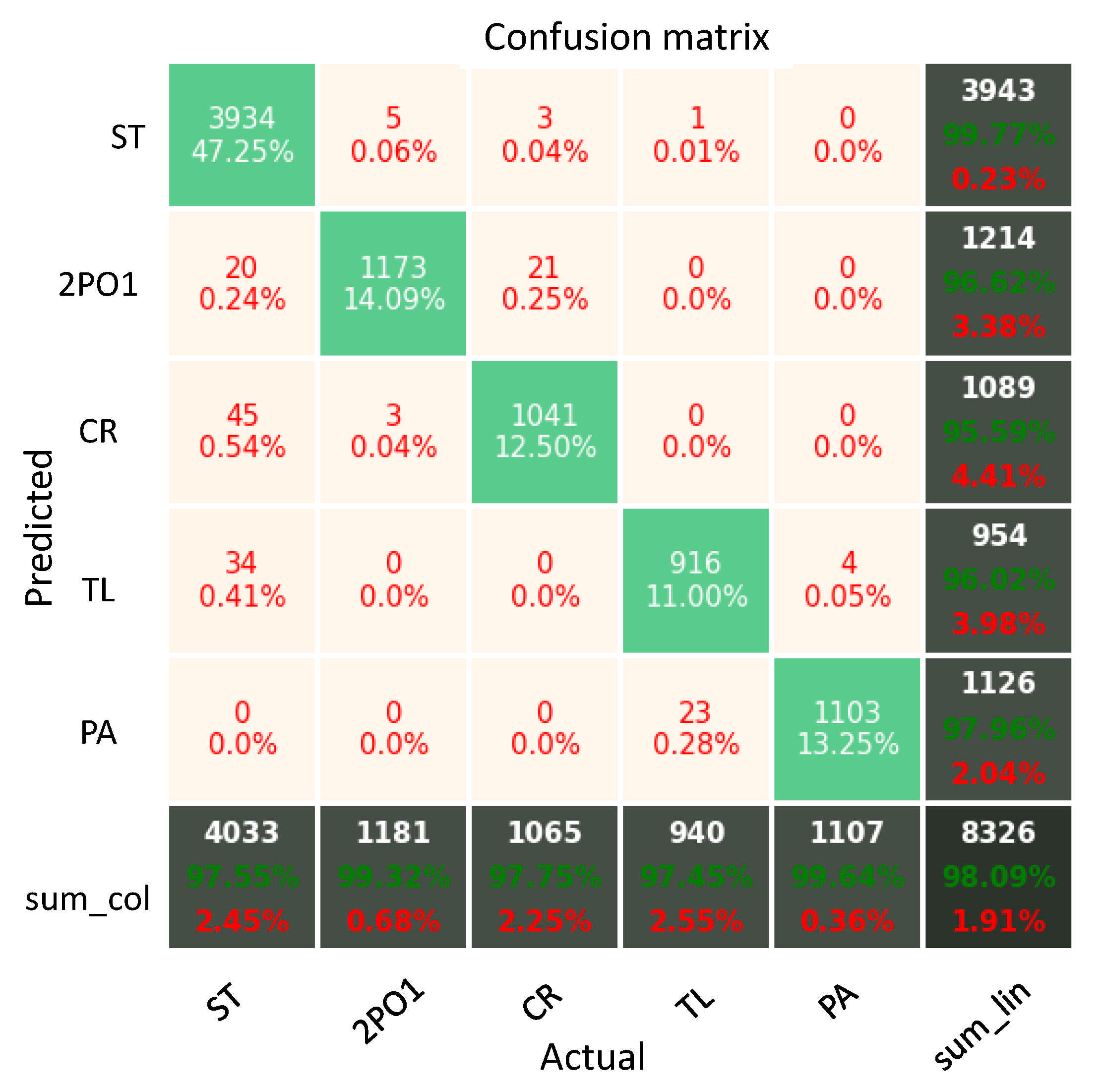
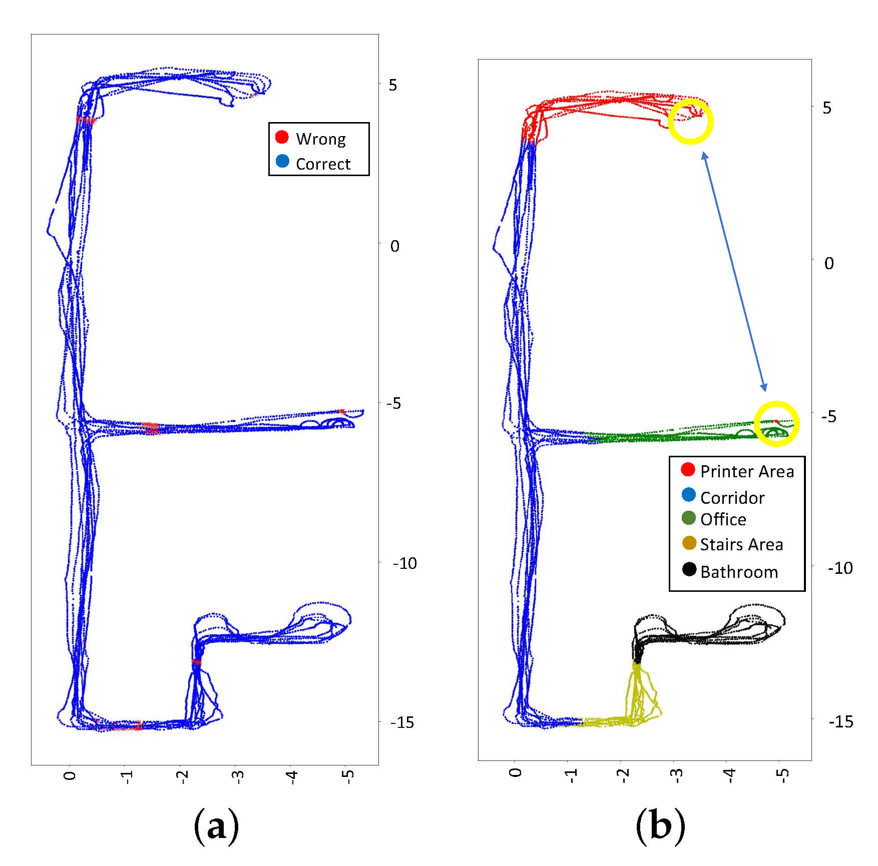
5.1.2. Results of the Classification CNN

Once the training is completed by using the augmented cloudy dataset, the resultant CNN was evaluated and the accuracy reached was 98.11% (i.e., percentage of times that the trained CNN retrieves correctly the room from which the input image was captured). Figure 2 shows the confusion matrix obtained. From this figure, the conclusion reached is that despite the fact that some errors appear, they are mostly due to confusions with images captured in transition areas between different rooms. For example, images from the corridor are retrieved as printer area, office and stairs area (which are adjacent to the corridor), but they are never predicted as toilet (which is totally disconnected from the corridor). Nonetheless, 21 images from the office room were retrieved as printer area despite the fact that those rooms are not adjacent. This may be due to the appearance similarity between them. Despite these few mistakes, the hit rate is significantly high. The high accuracy rate is noticed more clearly in the trajectory maps shown in Figure 3. First, Figure 3a shows the capture point of each test image with blue color, in case that the CNN correctly retrieves the room and with red color in case of wrong retrieval. Second, Figure 3b shows these capture points with different colors that indicate the room that the CNN has retrieved for each test image. Hence, from these results, the conclusion is that the CNN is properly trained to tackle the room retrieval task.

5.2. Results of the Fine Localization Stage

This section focuses on the fine localization of the robot. Once the classification CNN identifies the room where the robot is located, the regression CNN of this room is selected to obtain the fine localization of the robot, i.e., its X and Y coordinates. This section presents the results obtained in the second stage (fine localization). Section 5.2.1 presents the details of the training of the regression CNNs and Section 5.2.2 shows the results obtained in the fine localization stage.

5.2.1. Training Process of the Regression CNNs

In the present subsection, instead of a classification task, we focus on addressing a regression task. That is, once the CNN is properly trained for room retrieval purposes, the next step consists in carrying out the transfer learning and re-training of the network with the aim of estimating the position of the robot in the ground plane (i.e., the coordinates X, Y). In this sense, since the network was designed for classification, it is necessary to carry out some modifications in the architecture. Moreover, a new network is developed for each room and, in some cases, several networks for different parts of a single room, with the aim of improving the performance, as explained later in this section. The objective output of the network is not a one-hot vector, but two values: coordinate X and coordinate Y. Hence, the labeling should be adapted for the new training. The coordinates will be output through two perceptrons with the aim of fitting best each one to its loss function. Additionally, the labels will be normalized, since the different ranges of the coordinates could affect the weights of the final error function. The labels for training are the X and Y coordinates, obtained from the ground truth of the database. The normalization procedure is performed independently for each coordinate and for each room. These values are ranged between 0 and 1.
Concerning the transfer learning, as explained in previous sections, this technique is useful to save training time, since the most of the layers are already tuned to address a similar problem. In this case, the previous CNN was trained with the aim of obtaining robust holistic descriptors from the omnidirectional images and then use that information to carry out a classification (room retrieval) task, as shown in Section 5.1.2. In this new task, the objective consists in using the feature information to estimate the coordinates of the capture point of the test image. Therefore, the featuring part of the CNN can be kept and only the classification part is modified. Figure 4 shows the the architecture that we use to perform the regression task. It is obtained after applying the proposed changes to the CNN developed for room retrieval (transfer learning). In this figure, we show with green color the layers that are kept from the classification CNN (both these layers and their parameters are kept), and with blue color the layers that are changed from the original classification CNN to obtain the regression CNN.

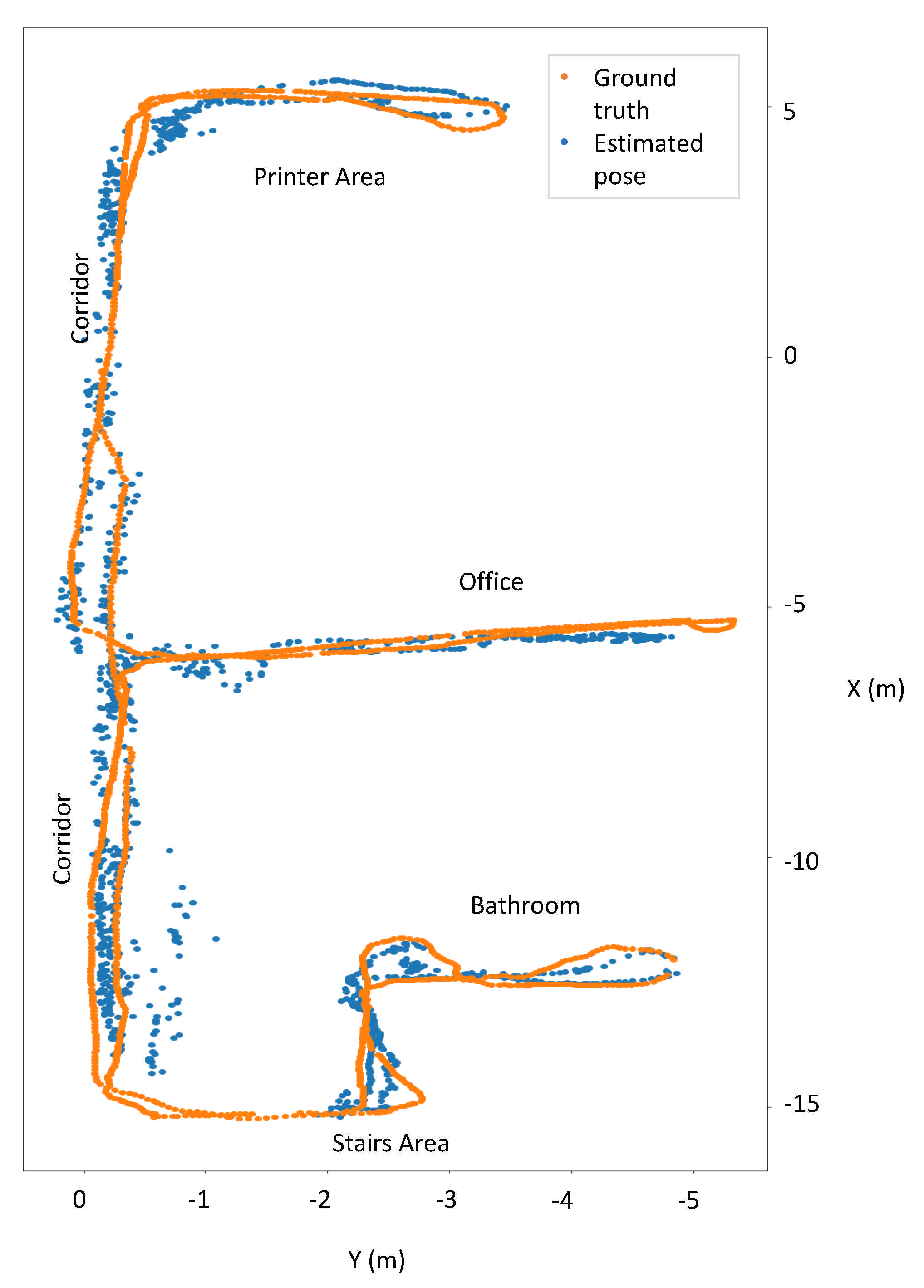
5.2.2. Results of the Regression CNNs

After training the networks, their performances were analyzed and the localization results are summed up in Table 3. Additionally, to assess the performance of the method, the following values are included in the table: the average, maximum and minimum error, along the X-axis, along the Y-axis and global (error measured as Euclidean distance). Additionally, the deviation of the error is included in the table. The X and Y axes can be seen in Figure 5. Regarding the performance for the stairs area, the X coordinate results are good, but the Y coordinates are worse, because they reach extreme values. Nevertheless, the deviation value is low, and hence the extreme values can be aisle cases. Concerning the performance related to the toilet, the average error is similar for both coordinates and they are relatively low. The deviation values are also low. Hence, the CNN trained for this room exhibits good performances. As for the corridor, the table shows that despite the low average error values, there are extreme error values. This is also noticed by observing the deviation values. From these results, it is concluded that this room needs a special treatment with the aim of obtaining a network capable of addressing the pose estimation more accurately. Regarding the printer area, the related error values are accurate enough, since the average error for the euclidean distance is around 30 cm and the training images presented an average distance of 20 cm. Furthermore, the deviation values are not significantly high. Last, concerning the office, the results shown in the Table 3 are not good enough if we take into consideration the size of this room. This drawback can be introduced because the trajectory addressed by the robot in the test dataset differs substantially from the trajectory addressed during the training.
Table 3 also shows a column with the average results for the five rooms. Moreover, Figure 5 shows the trajectory map of the ground truth data and the pose estimations provided by the CNNs. In general, pose predictions fit real poses. There are critical results concerning the office and the extreme parts of the corridor. In these areas, the predictions are significantly inaccurate. Therefore, improvements should be addressed in those two rooms.

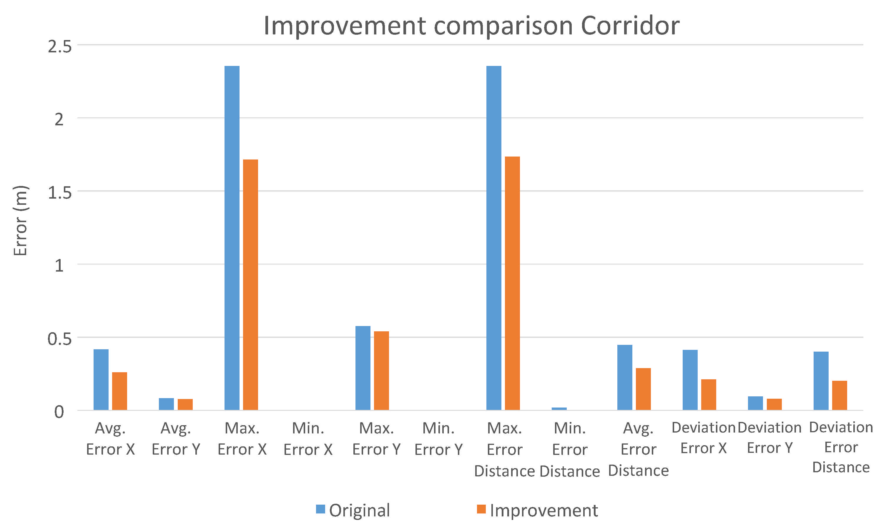
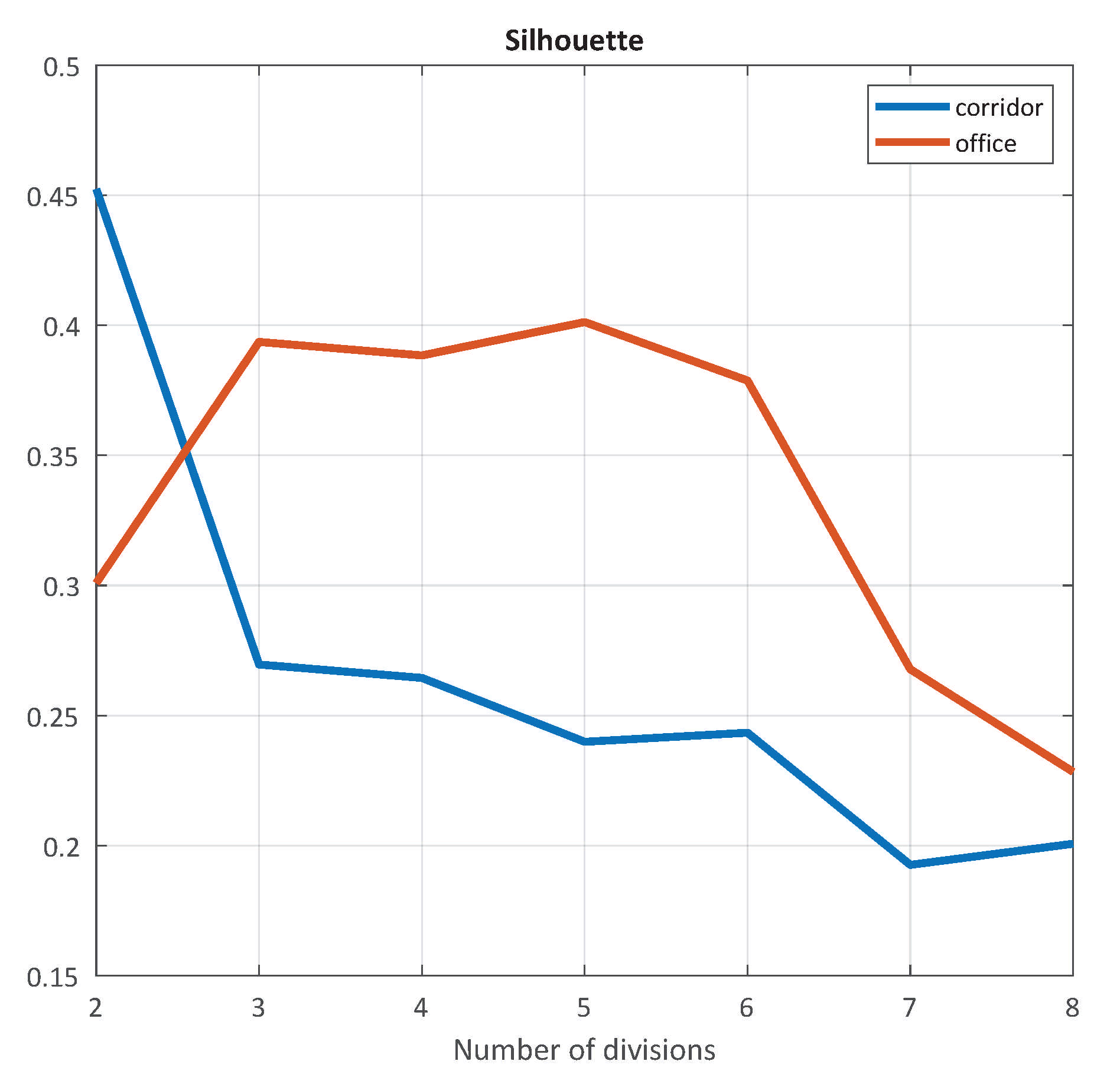
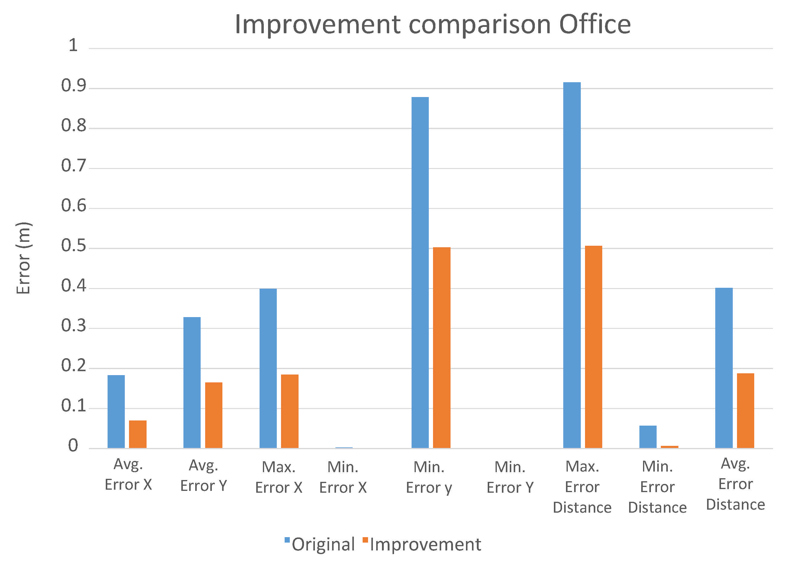
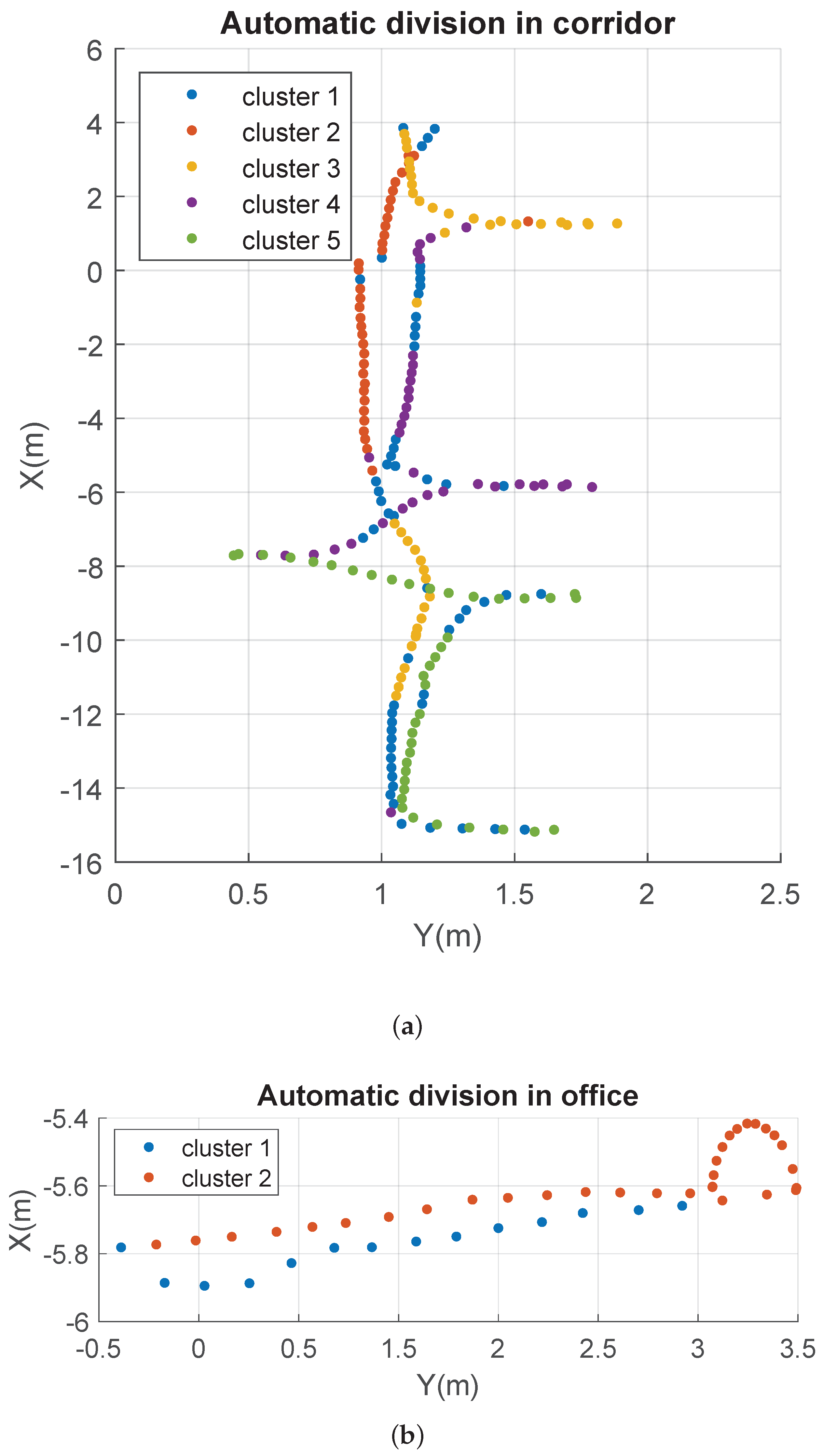
5.2.3. Improvement of the Regression CNNs

As presented above, after analyzing the results output by the regression CNNs, the networks of some of the rooms are not able to provide successful position estimations. Therefore, the aim of the present subsection is to propose some additional operations to improve the results. This subsection focuses on improving the regression CNNs related to the corridor and the office, since their related results were the worst among all the rooms within the environment.
First, regarding the office, Figure 5 shows that the trajectory in this room is mainly distributed along the Y-axis (and therefore, the error along this axis is relative high, as shown in Table 3). Taking this fact into account, we propose splitting this room into two zones. An automatic splitting has been used by applying a spectral clustering approach in a similar way as it was done in [48]. After addressing the split, two regression CNNs were independently trained to carry out the position estimation task in each of the two zones. As for the room retrieval, two alternatives can be given: either retraining the classification CNN considering the office as two independent rooms (i.e., considering six rooms in total), or applying an intermediate step which retrieves the proper part of the office after retrieving the room and before estimating the robot position within the room. The results obtained are shown in Figure 6. From it, the conclusion reached is that the results obtained by applying a room division present a significant error reduction.
Concerning the corridor room, the main errors were observed along the X axis. Hence, in this case, similar to the solution presented for the office room, an automatic split of the room is addressed by means of a spectral clustering method. Due to the length of this room, it was split into five areas.
After carrying out the division and training of the regression CNNs (one per area), the pose estimation is performed in the corridor room. The results are shown in the Figure 7. From it, the conclusion reached is that the errors are considerably reduced. Despite the fact that the average error has been reduced, the maximum error is still relatively high. Furthermore, the standard deviation has also been reduced; hence, there is a lower number of extreme cases. This room division presents an improvement along the X axis.
To evaluate the quality of the groups of images considered in this splitting strategy, the silhouette parameter is considered. It provides information about how compact the clusters are, that is, the silhouette parameter measures the degree of similarity between the instances within the same cluster and at the same time the dissimilarity with the instances which belong to others clusters. The values are in the range [ 1 , 1 ] and the higher it is, the more compact the clusters are. Figure 8 shows the silhouettes values obtained for office and corridor for a number of divisions between 2 and 8. As we can observe, the maximum values are reached for 2 and 5 divisions, respectively. In addition, Figure 9 shows the labeling made by the spectral clustering approach in office and corridor. This information is processed according the axis of interest (Y for office and X for corridor) and then, the splitting of the information is carried out, respectively, on the axis of interest.

6. Conclusions and Future Works

This paper presents a study about the use of CNNs to carry out the hierarchical localization by means of omnidirectional images in indoor environments. A classification CNN is trained to address the room retrieval by using a transfer learning technique. Additionally, transfer learning is used again to transform the CNN in a regression CNN and thus addressing the pose estimation within a specific room. The architecture of the network used produces acceptable results regarding accuracy and training time. The results obtained for the room retrieval task are considerably successful, since the percentage of success is 98.11% and the majority of the few confusions are given in the frontiers between different rooms.
As for the regression CNN, the initial results cannot be considered accurate, since considerable errors arise in some specific rooms, such as the corridor. Nonetheless, after applying an improvement strategy based on splitting in areas those rooms in which the robot runs a long, linear trajectory, the new networks are able to output more accurate results.
Concerning the improvement of the regression CNNs, several alternatives could be considered in future works to continue improving the results. On the one hand, splitting the rooms into smaller areas (subrooms) and generating more training images by a data augmentation technique, in such a way that the networks are more robustly trained to estimate the position of the robot in each room. On the other hand, the pose estimation could be addressed by using recurrent networks instead of regression networks. In this way, the current position of the robot within the room would be estimated considering the previously estimated poses. Additionally, using more recent CNN architectures could permit extracting more robust features and then the regression network could provide better results.
Finally, other future research lines include the performance of the proposed method with other datasets whose environments present different challenges, such as outdoor environments or different capturing strategies. Moreover, a hierarchical localization approach based on Long Short Term Memory (LSTM) networks will be developed.

Author Contributions

Conceptualization, M.B. and L.P.; methodology, L.P.; software, S.C. and F.M.; validation, S.C., M.B. and O.R.; formal analysis, O.R. and L.P.; investigation, S.C. and M.B.; resources, M.B. and L.P.; data curation, L.P.; writing—original draft preparation, S.C. and M.B.; writing—review and editing, M.B., L.P. and O.R.; visualization, F.M.; supervision, M.B.; project administration, M.B. and O.R.; funding acquisition, M.B. and O.R. All authors have read and agreed to the published version of the manuscript.

Funding

This work has been supported by the Spanish government through the project PID2020-116418RB-I00: “HYREBOT: Robots híbridos y reconstrucción multisensorial para aplicaciones en estructuras reticulares”.

Data Availability Statement

Publicly available datasets were analyzed in this study. This data can be found here: https://www.cas.kth.se/COLD/cold-freiburg.html (accessed on 6 August 2021).

Conflicts of Interest

The authors declare no conflict of interest.

References

  1. Hamid, M.; Adom, A.; Rahim, N.; Rahiman, M. Navigation of mobile robot using Global Positioning System (GPS) and obstacle avoidance system with commanded loop daisy chaining application method. In Proceedings of the 2009 5th International Colloquium on Signal Processing Its Applications, Kuala Lumpur, Malaysia, 6–8 March 2009; pp. 176–181. [Google Scholar] [CrossRef]
  2. Markom, M.A.; Adom, A.H.; Tan, E.S.M.M.; Shukor, S.A.A.; Rahim, N.A.; Shakaff, A.Y.M. A mapping mobile robot using RP Lidar scanner. In Proceedings of the 2015 IEEE International Symposium on Robotics and Intelligent Sensors (IRIS), Langkawi, Malaysia, 18–20 October 2015; pp. 87–92. [Google Scholar] [CrossRef]
  3. Almansa-Valverde, S.; Castillo, J.C.; Fernández-Caballero, A. Mobile robot map building from time-of-flight camera. Expert Syst. Appl. 2012, 39, 8835–8843. [Google Scholar] [CrossRef] [Green Version]
  4. Jiang, G.; Yin, L.; Jin, S.; Tian, C.; Ma, X.; Ou, Y. A Simultaneous Localization and Mapping (SLAM) Framework for 2.5D Map Building Based on Low-Cost LiDAR and Vision Fusion. Appl. Sci. 2019, 9, 2105. [Google Scholar] [CrossRef] [Green Version]
  5. Ballesta, M.; Gil, A.; Reinoso, O.; Payá, L. Building Visual Maps with a Team of Mobile Robots; INTECHOpen: London, UK, 2011; Chapter 6. [Google Scholar] [CrossRef] [Green Version]
  6. Se, S.; Lowe, D.; Little, J. Vision-based mobile robot localization and mapping using scale-invariant features. In Proceedings of the 2001 ICRA. IEEE International Conference on Robotics and Automation, Seoul, Korea, 21–26 May 2001; Volume 2, pp. 2051–2058. [Google Scholar] [CrossRef] [Green Version]
  7. Gil, A.; Reinoso, O.; Ballesta, M.; Juliá, M.; Payá, L. Estimation of Visual Maps with a Robot Network Equipped with Vision Sensors. Sensors 2010, 10, 5209–5232. [Google Scholar] [CrossRef] [PubMed]
  8. Ali, S.; Al Mamun, S.; Fukuda, H.; Lam, A.; Kobayashi, Y.; Kuno, Y. Smart Robotic Wheelchair for Bus Boarding Using CNN Combined with Hough Transforms; In International Conference on Intelligent Computing; Springer: Cham, Switzerland, 2018; pp. 163–172. [Google Scholar] [CrossRef]
  9. Khan, A.; Sohail, A.; Zahoora, U.; Saeed, A. A Survey of the Recent Architectures of Deep Convolutional Neural Networks. Artif. Intell. Rev. 2020, 53, 5455–5516. [Google Scholar] [CrossRef] [Green Version]
  10. Andreasson, H. Local Visual Feature Based Localisation and Mapping by Mobile Robots. Ph.D. Thesis, Örebro University, Örebro, Sweden, 2008. ISSN 1650-8580 ISBN 978-91-7668-614-0. [Google Scholar]
  11. Ravankar, A.A.; Ravankar, A.; Emaru, T.; Kobayashi, Y. Multi-Robot Mapping and Navigation Using Topological Features. Proceedings 2020, 42, 6580. [Google Scholar] [CrossRef] [Green Version]
  12. Lowe, D. Object Recognition from Local Scale-Invariant Features. Proc. IEEE Int. Conf. Comput. Vis. 2001, 2, 1150–1157. [Google Scholar]
  13. Bay, H.; Ess, A.; Tuytelaars, T.; Van Gool, L. Speeded-Up Robust Features (SURF). Comput. Vis. Image Underst. 2008, 110, 346–359. [Google Scholar] [CrossRef]
  14. Amorós, F.; Payá, L.; Mayol-Cuevas, W.; Jiménez, L.; Reinoso, O. Holistic Descriptors of Omnidirectional Color Images and Their Performance in Estimation of Position and Orientation. IEEE Access 2020, 8, 81822–81848. [Google Scholar] [CrossRef]
  15. Abdi, H.; Williams, L. Principal Component Analysis. Wiley Interdiscip. Rev. Comput. Stat. 2010, 2, 433–459. [Google Scholar] [CrossRef]
  16. Huang, G.; Liu, Z.; Weinberger, K. Densely Connected Convolutional Networks. arXiv 2016, arXiv:1608.06993. [Google Scholar]
  17. Redmon, J.; Farhadi, A. YOLOv3: An Incremental Improvement. arXiv 2018, arXiv:1804.02767. [Google Scholar]
  18. Krizhevsky, A.; Sutskever, I.; Hinton, G.E. Imagenet classification with deep convolutional neural networks. Adv. Neural Inf. Process. Syst. 2017, 25, 1097–1105. [Google Scholar] [CrossRef]
  19. LeCun, Y.; Bengio, Y.; Hinton, G. Deep Learning. Nature 2015, 521, 436–444. [Google Scholar] [CrossRef]
  20. Szegedy, C.; Liu, W.; Jia, Y.; Sermanet, P.; Reed, S.; Anguelov, D.; Erhan, D.; Vanhoucke, V.; Rabinovich, A. Going deeper with convolutions. In Proceedings of the 2015 IEEE Conference on Computer Vision and Pattern Recognition (CVPR), Boston, MA, USA, 7–12 June 2015; pp. 1–9. [Google Scholar] [CrossRef] [Green Version]
  21. Taoufiq, S.; Nagy, B.; Benedek, C. HierarchyNet: Hierarchical CNN-Based Urban Building Classification. Remote Sens. 2020, 12, 3794. [Google Scholar] [CrossRef]
  22. Tanaka, M.; Umetani, T.; Hirono, H.; Wada, M.; Ito, M. Localization of Moving Robots By Using Omnidirectional Camera in State Space Framework. Proc. ISCIE Int. Symp. Stoch. Syst. Theory Its Appl. 2011, 2011, 19–26. [Google Scholar] [CrossRef] [Green Version]
  23. Huei-Yung, L.; Chien-Hsing, H. Mobile Robot Self-Localization Using Omnidirectional Vision with Feature Matching from Real and Virtual Spaces. Appl. Sci. 2021, 11, 3360. [Google Scholar] [CrossRef]
  24. Ishii, M.; Sasaki, Y. Mobile Robot Localization through Unsupervised Learning using Omnidirectional Images. J. Jpn. Soc. Fuzzy Theory Intell. Inform. 2015, 27, 757–770. [Google Scholar] [CrossRef] [Green Version]
  25. Cebollada, S.; Payá, L.; Juliá, M.; Holloway, M.; Reinoso, Ó. Mapping and localization module in a mobile robot for insulating building crawl spaces. Autom. Constr. 2018, 87, 248–262. [Google Scholar] [CrossRef]
  26. LeCun, Y.; Boser, B.; Denker, J.S.; Henderson, D.; Howard, R.E.; Hubbard, W.; Jackel, L.D. Backpropagation Applied to Handwritten Zip Code Recognition. Neural Comput. 1989, 1, 541–551. [Google Scholar] [CrossRef]
  27. Lecun, Y.; Bottou, L.; Bengio, Y.; Haffner, P. Gradient-based learning applied to document recognition. Proc. IEEE 1998, 86, 2278–2324. [Google Scholar] [CrossRef] [Green Version]
  28. He, K.; Zhang, X.; Ren, S.; Sun, J. Deep Residual Learning for Image Recognition. arXiv 2015, arXiv:1512.03385. [Google Scholar]
  29. Simonyan, K.; Zisserman, A. Very Deep Convolutional Networks for Large-Scale Image Recognition. arXiv 2014, arXiv:1409.1556. [Google Scholar]
  30. Szegedy, C.; Ioffe, S.; Vanhoucke, V. Inception-v4, Inception-ResNet and the Impact of Residual Connections on Learning. arXiv 2016, arXiv:1602.07261. [Google Scholar]
  31. Da Silva, S.P.P.; da Nòbrega, R.V.M.; Medeiros, A.G.; Marinho, L.B.; Almeida, J.S.; Filho, P.P.R. Localization of Mobile Robots with Topological Maps and Classification with Reject Option using Convolutional Neural Networks in Omnidirectional Images. In Proceedings of the 2018 International Joint Conference on Neural Networks (IJCNN), Rio de Janeiro, Brazil, 8–13 July 2018; pp. 1–8. [Google Scholar] [CrossRef]
  32. Kim, K.W.; Hong, H.G.; Nam, G.P.; Park, K.R. A Study of Deep CNN-Based Classification of Open and Closed Eyes Using a Visible Light Camera Sensor. Sensors 2017, 17, 1534. [Google Scholar] [CrossRef] [PubMed] [Green Version]
  33. Cebollada, S.; Payá, L.; Román, V.; Reinoso, O. Hierarchical Localization in Topological Models Under Varying Illumination Using Holistic Visual Descriptors. IEEE Access 2019, 7, 49580–49595. [Google Scholar] [CrossRef]
  34. Kanezaki, A.; Matsushita, Y.; Nishida, Y. Rotationnet: Joint object categorization and pose estimation using multiviews from unsupervised viewpoints. In Proceedings of the IEEE Conference on Computer Vision and Pattern Recognition, Salt Lake City, UT, USA, 18–23 June 2018; pp. 5010–5019. [Google Scholar]
  35. Sünderhauf, N.; Shirazi, S.; Dayoub, F.; Upcroft, B.; Milford, M. On the performance of ConvNet features for place recognition. In Proceedings of the IEEE International Conference on Intelligent Robots and Systems (IROS), Hamburg, Germany, 28 September–2 October 2015; pp. 4297–4304. [Google Scholar] [CrossRef] [Green Version]
  36. Girshick, R.; Donahue, J.; Darrell, T.; Malik, J. Rich feature hierarchies for accurate object detection and semantic segmentation. In Proceedings of the IEEE Conference on Computer Vision and Pattern Recognition, Columbus, OH, USA, 23–28 June 2014; pp. 580–587. [Google Scholar]
  37. Girshick, R. Fast r-cnn. In Proceedings of the IEEE International Conference on Computer Vision, Santiago, Chile, 13–16 December 2015; pp. 1440–1448. [Google Scholar]
  38. Ren, S.; He, K.; Girshick, R.; Sun, J. Faster r-cnn: Towards real-time object detection with region proposal networks. Adv. Neural Inf. Process. Syst. 2015, 28, 91–99. [Google Scholar] [CrossRef] [PubMed] [Green Version]
  39. He, K.; Gkioxari, G.; Dollár, P.; Girshick, R. Mask r-cnn. In Proceedings of the International Conference on Computer Vision, Venice, Italy, 22–29 October 2017; pp. 2961–2969. [Google Scholar]
  40. Kunii, Y.; Kovacs, G.; Hoshi, N. Mobile robot navigation in natural environments using robust object tracking. In Proceedings of the IEEE 26th International Symposium on Industrial Electronics (ISIE), Edinburgh, UK, 19–21 June 2017; pp. 1747–1752. [Google Scholar]
  41. Payá, L.; Reinoso, O.; Berenguer, Y.; Úbeda, D. Using omnidirectional vision to create a model of the environment: A comparative evaluation of global-appearance descriptors. J. Sens. 2016, 2016, 1209507. [Google Scholar] [CrossRef] [PubMed] [Green Version]
  42. Sinha, H.; Patrikar, J.; Dhekane, E.G.; Pandey, G.; Kothari, M. Convolutional Neural Network Based Sensors for Mobile Robot Relocalization. In Proceedings of the 23rd International Conference on Methods Models in Automation Robotics (MMAR), Miedzyzdroje, Poland, 27–30 August 2018; pp. 774–779. [Google Scholar] [CrossRef]
  43. Payá, L.; Peidró, A.; Amorós, F.; Valiente, D.; Reinoso, O. Modeling Environments Hierarchically with Omnidirectional Imaging and Global-Appearance Descriptors. Remote Sens. 2018, 10, 522. [Google Scholar] [CrossRef] [Green Version]
  44. Xu, S.; Chou, W.; Dong, H. A robust indoor localization system integrating visual localization aided by CNN-based image retrieval with Monte Carlo localization. Sensors 2019, 19, 249. [Google Scholar] [CrossRef] [Green Version]
  45. Chaves, D.; Ruiz-Sarmiento, J.; Petkov, N.; Gonzalez-Jimenez, J. Integration of CNN into a Robotic Architecture to Build Semantic Maps of Indoor Environments. In Proceedings of the Advances in Computational Intelligence, Gran Canaria, Spain, 12–14 June 2019; Springer International Publishing: Cham, Switzerland, 2019; pp. 313–324. [Google Scholar]
  46. Pronobis, A.; Caputo, B. COLD: COsy Localization Database. Int. J. Robot. Res. 2009, 28, 588–594. [Google Scholar] [CrossRef] [Green Version]
  47. COsy Localization Database. Available online: https://www.cas.kth.se/COLD/cold-freiburg.html (accessed on 21 July 2021).
  48. Cebollada, S.; Payá, L.; Mayol, W.; Reinoso, O. Evaluation of Clustering Methods in Compression of Topological Models and Visual Place Recognition Using Global Appearance Descriptors. Appl. Sci. 2019, 9, 377. [Google Scholar] [CrossRef] [Green Version]
Figure 1. Sample omnidirectional images from the Freiburg dataset, part A. The images were captured under (a) cloudy, (b) night and (c) sunny illumination conditions.
Applsci 11 07521 g001
Figure 2. Confusion matrix of the room retrieval classification. These results were obtained by using the trained CNN and the augmented dataset of images captured with cloudy illumination. The rows define the real room of the images and the columns the prediction addressed by the network.
Applsci 11 07521 g002
Figure 3. Trajectory maps. (a) The correct (blue) and the wrong (red) retrievals tackled by the developed CNN. (b) The room retrievals done along the trajectory. Each room has been assigned a different color (e.g., the red color indicates the images that have been retrieved by the CNN as belonging to the printer area). Apart from the expected mistakes in the transition areas, there is some confusion between the printer area (red color) and the office (green).
Applsci 11 07521 g003
Figure 4. Transfer learning process addressed from the CNN for the room retrieval task (left) to develop the CNN that estimates the the X , Y coordinates (right).
Applsci 11 07521 g004
Figure 5. Global representation of the coordinates. The orange points represent the ground truth and the blue points are the estimations made by the regression CNNs from each test image.
Applsci 11 07521 g005
Figure 6. Results for the office pose estimation reached by applying the proposed method to improve the accuracy of the regression CNN.
Applsci 11 07521 g006
Figure 7. Results for the office pose estimation reached by applying two improvement methods to increase the related regression CNN accuracy.
Applsci 11 07521 g007
Figure 8. Results of the divisions by means of a spectral clustering method for office and corridor.
Applsci 11 07521 g008
Figure 9. Clusters obtained with spectral clustering for (a) corridor with 5 divisions and (b) office with 2 divisions.
Applsci 11 07521 g009
Table 1. Number of images for each room and for each illumination condition.
CodeRoom NameNumber of Images
CloudySunnyNight
1-PAPrinter area692985716
2-CRCorridor247231322537
8-TLToilet683854645
9-STStairs area433652649
5-2PO1Office609745649
-Total488963685196
Table 2. Labeling transformation. The room information label is transformed to one-hot vector with the aim of addressing the CNN classification training.
CodeOne-Hot Vector
CR[1, 0, 0, 0, 0]
PA[0, 1, 0, 0, 0]
2PO1[0, 0, 1, 0, 0]
ST[0, 0, 0, 1, 0]
TL[0, 0, 0, 0, 1]
Table 3. Localization results performed by the regression CNNs. Results (errors in the estimation and deviations, as detailed in the left column) are presented separately for coordinate X and coordinate Y and globally for both coordinates (Euclidean distance).
Room
StairsToiletCorridorPrinter AreaOfficeAverage
Average error X (m)0.07380.08230.87530.14660.18280.4523
Average error Y (m)0.10330.08140.09020.22450.3280.1452
Maximum error X (m)0.42540.49997.19010.43120.39917.1901
Minimum error X (m)0.00140.00050.000140.00120.00260.0001
Maximum error Y (m)0.7550.40610.57470.6520.87840.8784
Minimum error Y (m)0.00030.0001 5.52 × 10 5 0.0008 9.78 × 10 5 5.53 × 10 5
Maximum error Euclidean distance (m)0.75570.52077.19070.66060.91527.1907
Minimum error Euclidean distance (m)0.007680.0060.01690.03420.05690.006
Average error Euclidean distance (m)0.13981.3138.99202.92800.40110.5315
Error deviation in X (m)0.06780.08521.23020.10810.10340.8979
Error deviation in Y (m)0.13390.08130.09440.15140.21810.1586
Error deviation Euclidean distance (m)0.13820.10051.21990.1440.19610.8801
Publisher’s Note: MDPI stays neutral with regard to jurisdictional claims in published maps and institutional affiliations.

