Article

On IoT-Friendly Skewness Monitoring for Skewness-Aware Online Edge Learning

Department of Computer Science, University of Concepción, Concepción 4030000, Chile
*
Author to whom correspondence should be addressed.
Appl. Sci. 2021, 11(16), 7461; https://doi.org/10.3390/app11167461
Submission received: 26 July 2021 / Revised: 8 August 2021 / Accepted: 11 August 2021 / Published: 13 August 2021
(This article belongs to the Section Electrical, Electronics and Communications Engineering)

Abstract

:
Machine learning techniques generally require or assume balanced datasets. Skewed data can make machine learning systems never function properly, no matter how carefully the parameter tuning is conducted. Thus, a common solution to the problem of high skewness is to pre-process data (e.g., log transformation) before applying machine learning to deal with real-world problems. Nevertheless, this pre-processing strategy cannot be employed for online machine learning, especially in the context of edge computing, because it is barely possible to foresee and store the continuous data flow on IoT devices on the edge. Thus, it will be crucial and valuable to enable skewness monitoring in real time. Unfortunately, there exists a surprising gap between practitioners’ needs and scientific research in running statistics for monitoring real-time skewness, not to mention the lack of suitable remedies for skewed data at runtime. Inspired by Welford’s algorithm, which is the most efficient approach to calculating running variance, this research developed efficient calculation methods for three versions of running skewness. These methods can conveniently be implemented as skewness monitoring modules that are affordable for IoT devices in different edge learning scenarios. Such an IoT-friendly skewness monitoring eventually acts a cornerstone for developing the research field of skewness-aware online edge learning. By initially validating the usefulness and significance of skewness awareness in edge learning implementations, we also argue that conjoint research efforts from relevant communities are needed to boost this promising research field.

1. Introduction

Skewness measures the asymmetry of a probability distribution against the normal distribution, which plays a crucial role in the data-intensive machine learning implementations. From the perspective of exploitation, skewness can act as one of the statistical and representative features of datasets for building machine learning models [1,2]. In a special case, the skewness values of different datasets are even utilized as a boundary detection reference to facilitate clustering [3]. From the perspective of adverse effects, high skewness in training datasets can result in poor learning models that will make wrong estimation in prediction tasks [4,5]. In fact, it has been identified that machine learning models can never work well with skewed data, no matter how comprehensive their parameter tuning is [6]. Therefore, it is valuable and often necessary for both practitioners and machine learning systems to be aware of data skewness, so as, for example, to mitigate the negative influence of skewed data on model training [7].
When it comes to calculating skewness, according to the modern software systems of statistics, the most widely employed method is the adjusted Fisher–Pearson skewness coefficient [8,9], as formulated in Equation (1).
S = n ( n 1 ) ( n 2 ) · i = 1 n ( x i x ¯ ) 3 s 3
where S represents the skewness of sample data x 1 , x 2 , , x n , while x ¯ and s are the mean and standard deviation of the n samples respectively.
By using Equation (1), it is clear that the skewness calculation requires all the historical data. However, this methodof skewness calculation can be impractical in IoT and edge environments. Firstly, due to the limited storage capability of IoT devices, it would be impossible or expensive to keep all the collected data on the edge [10]. Secondly and more importantly, given continuous data flows at the edge side, the monitoring inevitably needs frequent skewness updates, while using Equation (1) to frequently obtain skewness values will be extremely inefficient due to the heavily repeated calculations and the limited computing capability of IoT and edge devices [11,12].
Therefore, the online skewness monitoring must resort to a real-time calculation strategy that fits in the characteristics of running statistics [13]. Unlike the standard method of skewness calculation, a running method should be able to recursively update skewness without storing the historical data. It should be noted that this recursive feature naturally matches the requirement of online machine learning. Surprisingly, there seems to be a lack of suitable skewness formulas or algorithms that can satisfy the various needs of skewness-aware online learning techniques. It is then no wonder that little work on skewness-aware online learning has been reported in the literature. For example, to our best knowledge, there is no practical running skewness method to work with the forgetting mechanism in the modern edge learning proposals (e.g., [14]). Although we can use a rolling window to “forget” old data, the typical approach to updating skewness is to supplement a negative datum of the tail when the data window moves ahead, (see the function remove() at https://github.com/alexander-yu/stream/blob/master/moment/core.go, accessed on 10 August 2021), and eventually it doubles both the calculation workload and the execution time. In the simplest case, the cumulative version of running skewness from several mathematical libraries can work for the basic online sequential learning (e.g., [15]). Nevertheless, we find that the corresponding algorithms are either inefficient or improper for skewness monitoring on the edge (cf. Section 4.3.3 and Section 4.3.4).
After observing frequent inquiries about running skewness in the open source community [16,17,18], we further affirmed the gap between practitioners’ needs and the scientific research on this topic. In detail, by studying the existing running skewness algorithms and the relevant statistical methods (i.e., running mean and running variance), we identified that the currently inefficient algorithms of cumulative running skewness are due to the inefficient calculation of running variance. Meanwhile, the missing of the other running skewness versions is mainly due to the lack of an efficient (or concise) cumulative version. Driven by these findings, this research develops IoT-friendly equation systems for calculating three popular running skewness versions and initially validates the usefulness and significance of skewness awareness in the implementation of online edge learning.
Correspondingly, this research makes a fourfold contribution:
  • From the statistics community’s perspective, this research enriches skewness monitoring solutions in the running statistics domain. It is worth highlighting that our solutions can conveniently be implemented into efficient algorithms and deployed on IoT devices for practical usage. In fact, compared with the pervasive discussions about mean, median, and variance (or standard deviation), skewness has been considered “a forgotten statistic” [8], not to mention running skewness. In particular, this research reminds the statistics community of the real-world needs of running skewness in the context of IoT and edge learning.
  • From the machine learning community’s perspective, this research paves the way for developing skewness-aware online learning techniques, which is particularly valuable and useful in the edge computing domain. It should be noted that although traditional skewness-aware machine learning has been studied [5,19], their generic strategy of curing high skewness (i.e., data pre-processing) cannot be applied to the online mode. In particular, this research reminds the machine learning community of the significance and the available methods of online skewness monitoring. After all, the slightest difference at the model training stage can lead to a huge error in the machine learning results.
  • In addition, the shared formula derivation details (in Appendix A) can help both researchers and practitioners investigate other versions of running skewness and develop corresponding algorithms, so as to satisfy the diverse needs in practice. It should be noted that not only has our work developed an efficient cumulative version of running skewness, but we have also investigated the other two versions that can satisfy the forgetting mechanism in the modern edge learning proposals. This contribution essentially follows the spirit of open methods that can act “as a higher-level strategy over open-source tools and open-access data” to facilitate scientific work [20]. In fact, this research has revealed that the obscurity in some advanced statistical methods may hinder their recognition and employment (cf. Section 3.1.2).
  • Overall, our work advocates and fosters cross-community research efforts on IoT-friendly online edge learning. Given the booming of edge intelligence [21] accompanied with the resource limits of IoT equipment (e.g., the embedded RAM is only 4KB in the current taxi-mounted GPS devices), multi-domain knowledge and expertise need to fuse together to address the challenges of online edge learning. Through this paper, we particularly expect to attract more attention from the statistics community and to inspire more skewness monitoring algorithms and techniques for the various needs in the diverse edge environments.
The remainder of this paper is organized as follows. Section 2 briefly reviews the background of online machine learning in edge computing, and discusses the research gap in skewness-aware online learning. Section 3 specifies the IoT-friendly equation systems of the three versions of running skewness. For the ease of reading, their derivation details are separately shared in Appendix A. Section 4 particularly focuses on the cumulative version of running skewness and reports its algorithm performance evaluation, while the evaluation result is representative for all the three versions of running skewness. Section 5 initially validates the usefulness of applying skewness monitoring to online learning implementations. The conclusions are drawn in Section 6, together with our future work plans.

2. Related Work

The proliferation and interconnection of numerous data sources across various IoT devices are speeding up the digital explosion in our everyday lives [22]. For example, the International Data Corporation estimates that about 80 billion devices will be connected to the Internet by 2025, and as a result, the globally generated data will be as tremendous as 163 zettabytes [23]. Since it is often impractical and even impossible to centralize the explosive data due to the bandwidth limits and privacy concerns, some research organization have predicted that the majority of the data (over 90 percent) will be stored and processed locally in a distributed manner [24]. Correspondingly, along with the revolutionary development of ubiquitous mobile equipment, wearable gadgets and smart sensors, innovative data analytical solutions are increasingly developed and deployed on the edge of the Internet.
In particular, driven by the intensive interests in the “intelligent edge” [23], there is a clear trend in implementing machine learning techniques on various and distributed IoT devices on the edge. Although the implementation of edge machine learning is still at an early stage [25], it is evident that IoT and edge devices are complementary to cloud resources for scaling machine learning systems [24]. Furthermore, considering that the data in production for edge learning are generated gradually instead of being available all at once, the trained models must be updated “in an online fashion to accommodate new data without compromising its performance on old data” [26]. Thus, online machine learning has become a distinctive research topic in the edge learning field [27], which can be characterized by the real-time streaming processing computation model [28].
In fact, the revival of online learning in edge computing can be traced back to sequential learning, which was studied decades ago [29]. Nevertheless, as identified in [15], those early studies may still require (estimating) the samples’ statistical information in advance for their sequential learning implementations. On the other hand, although recent studies have tried to simplify the online learning mechanisms, the solutions seem to be bypassing, ignoring, or tolerating the missing of the statistical characteristics of data, e.g., pre-setting suitable skewness values for simulations [30,31], using robust-to-skewness metrics to measure performance [32], etc.
It should be clarified that the machine learning community is well aware of the importance of skewness. For example, since canonical machine learning techniques assume balanced datasets [19], not only class skewness but also skewed features will bias the classification of dataset samples [33]. More generally, it has been identified that machine learning models cannot do a good job with skewed data, no matter how well the parameter tuning is conducted [6]. Unfortunately, to our best knowledge, little research into online machine learning has taken into account the real-time awareness of skewness. The study [34] is the only one we have found to monitor data skewness at runtime, which aims to balance the skewness of labels to train weak classifiers more equally. However, its skewness calculation is not compatible with the de facto adjusted Fisher–Pearson skewness coefficient (cf. Equation (1)). In addition, this use case only corresponds to the cumulative version of running skewness (cf. Section 3).
In contrast, this research investigates three running skewness versions and their calculation methods, by aligning with the adjusted Fisher–Pearson skewness coefficient. The proposed calculation methods can conveniently be converted into efficient algorithms and be implemented as skewness monitoring modules on IoT devices in order to satisfy the different needs of skewness-aware online edge learning.

3. Three Versions of Running Skewness and Efficient Calculation Methods

Given the continuous nature of online data flows, it is improper to assume online learning to be based on a complete data population. Therefore, we treat the processed data always to be samples, and correspondingly, we investigate the sample skewness instead of the population skewness of data. Furthermore, we take into account three versions of running skewness that may be the most useful ones for implementing skewness-aware online edge learning, such as the following:
  • RunningCumulative Sample Skewness recursively measures the skewness of the time series data filtered from the beginning of measurement up until the current moment. This skewness version is suitable for the situation when the individual data points in a time series are all equally important (e.g., [15]).
  • RunningRolling(Simple Moving)Sample Skewness recursively measures the skewness of the time series data within a fixed-size while continuously moving sample window. This skewness version is able to match the learning scenario in which each datum is valid only for a period of time (e.g., [35]).
  • RunningExponentially Weighted Sample Skewness also recursively and cumulatively measures the skewness of time series data. Different from the cumulative version, the data are accompanied with weighting factors that decrease exponentially as the data recede into the past. This skewness version would be more practical in the process industry [36] and in the financial sector, as the more recent data can better reflect the current system/market status.
To facilitate explaining and distinguishing between these skewness versions, we clarify the terminology used in this research. Firstly, we follow GNU’s naming convention to emphasise the recursive feature of running statistics by highlighting the term “Running” [13], because “Moving” also means the moving activity and might result in confusions from time to time (e.g., [16]). Secondly, since “rolling window” is widely used when describing the moving activity in the literature, we employ the term “Rolling” to characterize the second skewness version. Thirdly, we refer to “exponentially weighted sample statistics” [37] to shorten the name of the third skewness version. Overall, for both reference convenience and distinctiveness, we use Cumulative Sample Skewness (CSS), Rolling Sample Skewness (RSS), and Exponentially Weighted Sample Skewness (EWSS), respectively, to indicate the three running skewness versions in the rest of this paper.
Furthermore, to facilitate reading and verifying the equations presented in the rest of this paper, we summarise the relevant notations in Table 1.

3.1. Cumulative Sample Skewness (CSS)

In this research, the efficient calculation of CSS relies on the efficient intermediate steps for calculating running mean and running variance. To make the reasoning process clear to readers, this paper also includes and explains cumulative sample mean (CSM) and cumulative sample variance (CSV).

3.1.1. Calculation of Cumulative Sample Mean (CSM)

Following the previous naming convention, we define CSM as implying the recursive calculation of the arithmetic average of a random sample from some population, as shown in Equation (2).
x ¯ n + 1 = x ¯ n + x n + 1 x ¯ n n + 1 , x ¯ 0 = 0 , n > 0
where x ¯ n represents the sample mean of a time series of n observation values x 1 , x 2 , , x n , while x ¯ n + 1 indicates the updated sample mean after the new value x n + 1 joins the observation time series. Although the derivation of Equation (2) is straightforward, we still briefly report it in this paper (cf. Appendix A.1) for the purpose of completeness.

3.1.2. Calculation of Cumulative Sample Variance (CSV)

In practice, standard deviation is commonly used to measure how far a set of data spread out from their average value. In order to make the derivation concise, this research focuses on sample variance instead of sample standard deviation, as shown in the equation system (3). Note that the sample standard deviation can conveniently be obtained by taking the square root of the sample variance.
s n 2 = V n n 1 , V 0 = V 1 = 0 , n > 1 V n + 1 = V n + ( x n + 1 x ¯ n + 1 ) ( x n + 1 x ¯ n )
where s n is the sample standard deviation of n observation values x 1 , x 2 , , x n . The sample variance s n 2 is defined as a proportional function of the auxiliary variable V n that can be calculated in a recursive way, while V n essentially carries the crucial information of the second Central Moment, i.e.,  i = 1 n ( x i x ¯ n ) 2 .
Despite the usage of different notations, Equation System (3) is the same as the algorithm proposed by B. P. Welford in 1962 [38]. However, Welford’s algorithm does not seem to be widely recognised and employed, possibly because “it is not obvious that the method is correct even in exact arithmetic” [39]. As a result, the straightforward but inefficient formula of recursive variance is still frequently shared in the community [40,41,42]. Therefore, we have managed to go through the derivation of Equation System (3) and shared the details as proof in Appendix A.2.

3.1.3. Calculation of Cumulative Sample Skewness (CSS)

By trying to minimize the amount of multiplication and exponentiation from the coding’s perspective, we developed Equation System (4) to calculate CSS.
S n = n · S n ( n 1 ) ( n 2 ) · s n 3 , S 0 = S 1 = S 2 = 0 , n > 2 S n + 1 = S n 3 · ( x ¯ n + 1 x ¯ n ) · V n + ( V n + 1 V n ) [ x n + 1 x ¯ n + 1 ( x ¯ n + 1 x ¯ n ) ]
where S n is the sample skewness of n observation values x 1 , x 2 , , x n . In this equation system, S n is defined as a proportional function of the auxiliary variable S n that can be calculated in a recursive fashion, while S n essentially carries the crucial information of the third central moment, i.e.,  i = 1 n ( x i x ¯ n ) 3 .
It should be noted that ( x ¯ n + 1 x ¯ n ) and ( V n + 1 V n ) can directly be obtained from the intermediate results in Equation (2) and Equation System (3), respectively. To our best knowledge, this is the most efficient way to calculate CSS, as derived in Appendix A.3 and validated in Section 4.3.

3.2. Rolling Sample Skewness (RSS)

The calculation of RSS proposed in this research is based on the same derivation logic of CSS. Here we also include and specify the formulas of rolling sample mean (RSM) and rolling sample variance (RSV) to facilitate sharing the proof details of RSS. In particular, we introduce a special symbol n k to represent the most recent k items from a time series of n samples.

3.2.1. Calculation of Rolling Sample Mean (RSM)

Given the rolling window size k for a time series of observation values x 1 , x 2 , , x n , x n + 1 , their RSM can be calculated via Equation (5).
x ¯ n + 1 k = x ¯ n k + x n + 1 x o k , n k > 0
where x ¯ n k stands for the sample mean of the most recent k observation values x n k + 1 , x n k + 2 , , x n , while x ¯ n + 1 k indicates the updated sample mean after rolling the observation window to include the new value x n + 1 while removing the oldest one x o (i.e.,  x n k + 1 ). The brief derivation of Equation (5) is shared in Appendix A.4.

3.2.2. Calculation of Rolling Sample Variance (RSV)

Here we adapt Welford’s algorithm [38] of CSV (cf. Section 3.1.2) to the rolling window scenario. It is noteworthy that although the adaptation of Welford’s algorithm has been discussed in the open source community [43], there does not seem to be any consensus answer yet. The main reason could still be the little disclosure of derivation details of Welford’s algorithm.
Following the previous notations, we let RSV be recursively calculated via Equation System (6). To our best knowledge, this is the most efficient approach to calculating RSV, as it requires less multiplication operations than the other methods [44].
s n k 2 = V n k k 1 , n k > 1 V n + 1 k = V n k + ( x n + 1 x o ) ( x n + 1 + x o x ¯ n + 1 k x ¯ n k )
where s n k 2 denotes the sample variance of the most recent k observation values x n k + 1 , x n k + 2 , , x n ; and it can recursively be updated through its corresponding auxiliary variable V n k by rolling the observation window to include new values while removing the oldest ones. The derivation details of Equation System (6) are shared in Appendix A.5.

3.2.3. Calculation of Rolling Sample Skewness (RSS)

Through the derivation specified in Appendix A.6, we define the Equation System (7) to calculate RSS.
S n k = k · S n k ( k 1 ) ( k 2 ) · s n k 3 , n k > 2 S n + 1 k = S n k 3 · ( x ¯ n + 1 k x ¯ n k ) · V n k + ( x n + 1 x o ) [ ( x o x ¯ n k ) ( x o 2 x ¯ n + 1 k + x ¯ n k ) + ( x n + 1 x ¯ n + 1 k ) ( x n + 1 + x o 2 x ¯ n + 1 k ) ]
where S n k represents the sample skewness of the most recent k observation values x n k + 1 , x n k + 2 , , x n . When the observation window keeps rolling forward, the continuous update of S n k will be realized through the recursive calculations of the auxiliary variables V n k and S n k .
It should be noted that compared with the other peer formula forms, the multiplication operations in Equation System (7) have been minimized. When implementing algorithm from this equation system, the item 2 x ¯ n + 1 k should be further expanded, so as to reuse the intermediate results, for instance ( x n + 1 x ¯ n + 1 k ) and ( x o x ¯ n + 1 k ) .

3.3. Exponentially Weighted Sample Skewness (EWSS)

This research derives the calculation method of EWSS by referring to the formula form of CSS, i.e., Equation System (4). In other words, different formula forms of CSS will result in different calculation methods of EWSS. Given the efficiency in the CSS calculation (cf. Section 3.1.3), we claim that the EWSS method in this research is also efficient.
In particular, we argue for the relationship between exponentially weighted sample statistics and cumulative sample statistics by reusing the well-known derivation logic of exponentially weighted sample mean (EWSM) [36]. Thus, this paper also includes EWSM and exponentially weighted sample variance (EWSV) to facilitate explaining how we obtain the formula for calculating EWSS.

3.3.1. Calculation of Exponentially Weighted Sample Mean (EWSM)

As specified in Appendix A.7, Equation (8) for calculating EWSM is essentially a formula transformation from CSM.
x ¯ w ( n + 1 ) = ( 1 α ) · x ¯ w ( n ) + α · x n + 1 , n > 0 , α ( 0 , 1 )
where x ¯ w ( n ) represents the sample mean of a time series of n observation values x 1 , x 2 , , x n with exponentially decreasing weights, while x ¯ w ( n + 1 ) indicates the updated EWSM after the new value x n + 1 joins the observation time series. In particular, α is a constant coefficient between 0 and 1, and a bigger α discounts the contribution of older data faster in the EWSM calculation.

3.3.2. Calculation of Exponentially Weighted Sample Variance (EWSV)

Benefiting from the CSV formula (3), we define Equation (9) to calculate EWSV. Despite different notations, this equation is also available in the open source community [17].
s w ( n + 1 ) 2 = ( 1 β ) · s w ( n ) 2 + β · ( x n + 1 x ¯ w ( n + 1 ) ) ( x n + 1 x ¯ w ( n ) ) , n > 0 , β ( 0 , 1 )
where s w ( n ) 2 denotes the EWSV of a time series of n observations; s w ( n + 1 ) 2 represents the updated EWSV after a new observation x n + 1 joins the time series, and β is also defined as a constant coefficients between 0 and 1, for discounting the contribution of older data in the EWSV calculation. In addition, we further constrain the relation between α and β , as shown in Equation System (10) and explained in Appendix A.8 and Appendix A.9.

3.3.3. Calculation of Exponentially Weighted Sample Skewness (EWSS)

Following the same derivation strategy as specified in Appendix A.9, we obtain the equation system (10) for calculating EWSS.
1 α 1 β = 1 , α , β ( 0 , 1 ) , n > 0 ( 1 2 α ) · s w ( n + 1 ) 3 · S w ( n + 1 ) = ( 1 β ) ( 1 2 β ) · s w ( n ) 3 · S w ( n ) 3 · ( x ¯ w ( n + 1 ) x ¯ w ( n ) ) ( 1 β ) · s w ( n ) 2 + β · ( x n + 1 x ¯ w ( n + 1 ) ) ( x n + 1 x ¯ w ( n ) ) · [ x n + 1 x ¯ w ( n + 1 ) ( x ¯ w ( n + 1 ) x ¯ w ( n ) ) ]
where α and β are constant coefficients directly reused from Equations (8) and (9), respectively; S w ( n ) denotes the EWSS of a time series of n observations; and S w ( n + 1 ) is the updated EWSS after a new observation x n + 1 joins the time series.
Note that we intentionally deliver the current form of the EWSS formula in order to highlight the reusable intermediate results for algorithm design, e.g., ( 1 β ) · s w ( n ) 2 from Equation (9).

4. Algorithm Performance Evaluation

To verify the effectiveness and efficiency of our developed running skewness methods, we decided to compare them against the third-party methods reported in the open source community. However, as mentioned previously, we only found comparable counterparts for the cumulative version of running skewness i.e., CSS. Therefore, we conducted performance evaluation and comparison for CSS only. Considering that the cumulative version plays a fundamental role in developing the rolling window version and the exponentially weighted version (i.e., RSS is based on the derivation logic of CSS and EWSS is based on the formula form of CSS), the CSS evaluation results will still be able to represent the performance of RSS and EWSS.

4.1. The CSS Calculation Method from GNU Scientific Library

The first third-party method involved in our comparison is from GNU Scientific Library (GSL) (the source code is located in the folder rstat within the zipped library gsl-latest.tar.gz at https://www.gnu.org/software/gsl/, accessed on 10 August 2021). GSL is a well-known numerical library covering a wide range of mathematical routines in C language. At the time of this research, the stable version is GSL-2.6, released on 20 August 2019. To facilitate the contrast between the GSL method and ours, we abstract GSL’s source code into an equation system using our notations, as shown in (11).
x ¯ n + 1 = x ¯ n + x n + 1 x ¯ n n + 1 , x ¯ 0 = 0 , n > 0 M 2 n + 1 = M 2 n + n · ( x n + 1 x ¯ n ) 2 n + 1 , M 2 0 = 0 M 3 n + 1 = M 3 n 3 · x n + 1 x ¯ n n + 1 · M 2 n + n · ( n 1 ) ( n + 1 ) 2 · ( x n + 1 x ¯ n ) 3 , M 3 0 = 0 S n + 1 = ( n ) 3 n + 1 · M 3 n + 1 ( ( M 2 n + 1 ) 3
where x ¯ n and S n , respectively, represent the sample mean and sample skewness of n observation values x 1 , x 2 , , x n . x ¯ n + 1 and S n + 1 are the updated sample mean and sample skewness after a new value x n + 1 joins the observation dataset. (The equation of S n + 1 is extracted from the code Line 184 to Line 186 of rstat.c.) As for the auxiliary variables M 2 and M 3 , GSL generally defines Mk n = i = 1 n ( x i x ¯ n ) k (in gsl_rstat.h).
When it comes to designing algorithms from formulas, a popular and practical strategy is to save reusable intermediate results to minimize computational workloads and to speed up programs. Thus, compared to Equation System (11), the source code of GSL employs a set of temporary variables to reuse the intermediate results, as shown in Algorithm 1. It should be noted that the equation systems (4) and (11) require n > 2 and n > 1 respectively to avoid the error of division by zero. To ensure “apple-to-apple” performance comparison among different algorithms, we intentionally set n > 2 in the if statement in Algorithm 1.
Algorithm 1 Cumulative Sample Skewness in GSL
    Input: The incoming observation value x.
    Global Parameters: The current amount of observations n, the sample mean m e a n of the current observation values, and the current values of auxiliary variables M 2 and M 3 .
    Output: Cumulative sample skewness of the n + 1 observations.
1:
n n + 1     ▹ The new observation is counted.
2:
d e l t a x m e a n     ▹ i.e.,  ( x n + 1 x ¯ n ) in Equation System (11).
3:
d e l t a _ n d e l t a / n
4:
t e r m 1 d e l t a * d e l t a _ n * ( n 1 )     ▹ i.e.,  n · ( x n + 1 x ¯ n ) 2 n + 1 in Equation System (11).
5:
m e a n m e a n + d e l t a _ n
6:
M 3 M 3 3 * d e l t a _ n * M 2 + t e r m 1 * d e l t a _ n * ( n 2 )
7:
M 2 M 2 + t e r m 1     ▹ The if statement is originally “if ( n > 0 ) ” in GSL’s source code.
8:
if n > 2 and (optionally) not in a chunk then
9:
     f a c ( n 1 ) 3 / n
10:
    return  f a c * M 3 / ( M 2 ) 3
11:
else
12:
    return 0     ▹ Numeric 0 or Boolean false depending on contexts.
13:
end if

4.2. The CSS Calculation Method from a Go Library

Although not specified by GSL, according to Equation System (11), the GSL method corresponds to the Fisher–Pearson coefficient of skewness. To reinforce the comparison results, we further identified an online statistical library written in Go (GoL) (an open-source Go library for online statistical algorithms at https://github.com/alexander-yu/stream, accessed on 10 August 2021), which employed the adjusted Fisher–Pearson coefficient of skewness. Despite the generic algorithms [45] cited by GoL, we also extract a skewness-specific equation system from GoL’s source code, as shown in Equation System (12), in order to facilitate the formula comparison.
x ¯ n + 1 = x ¯ n + x n + 1 x ¯ n n + 1 , x ¯ 0 = 0 , n > 2 C 2 n + 1 = C 2 n + n · ( x n + 1 x ¯ n ) 2 n + 1 , C 2 0 = 0 C 3 n + 1 = C 3 n 3 · x n + 1 x ¯ n n + 1 · C 2 n + n · ( n 1 ) ( n + 1 ) 2 · ( x n + 1 x ¯ n ) 3 , C 3 0 = 0 S n + 1 = n · ( n + 1 ) n 1 · C 3 n + 1 n + 1 ( C 2 n + 1 n + 1 ) 3
In addition to the same notations x, x ¯ , and S used in Equation System (11), we define C 2 and C 3 as two auxiliary variables in this equation system, by referring to Core.sums [2] and Core.sums [3], respectively, in the source code of GoL. By contrasting between the equation systems (12) and (11), it is clear that C 2 and C 3 are exactly the same as M 2 and M 3 for tracking the second and the third central moments, while only the calculations of S n + 1 are different. (The equation for calculating S n + 1 in Equation System (12) is extracted from the code Line 96 to Line 105 of skewness.go at https://github.com/alexander-yu/stream/blob/master/moment/skewness.go, accessed on 10 August 2021).
Similarly, we follow GSL’s code optimisation strategy to describe the GoL method’s CSS calculation into Algorithm 2. Note that similar temporary variables are used in this algorithm. Moreover, we use C 2 / n and C 3 / n respectively to replace the calculations of variables variance and moment (i.e.,  n n + 1 · C 2 n and n n + 1 · C 2 n ) in the source code, for the convenience of algorithm comparison. This replacement does not have a negative impact on the representation of the original algorithm in GoL, because the simplified math operations have even improved the algorithm efficiency.
Algorithm 2 Cumulative Sample Skewness in GoL
    Input: The incoming observation value x.
    Global Parameters: The current amount of observations n, the sample mean m e a n of the current observation values, and the current values of auxiliary variables C 2 (i.e., Core.sums [2]) and C 3 (i.e., Core.sums [3]).
    Output: Cumulative sample skewness of the n + 1 observations.
1:
n n + 1     ▹ The new observation is counted.
2:
d e l t a x m e a n     ▹ i.e.,  ( x n + 1 x ¯ n ) in Equation System (12).
3:
d e l t a _ n d e l t a / n
4:
t e r m 1 d e l t a * d e l t a _ n * ( n 1 )     ▹ i.e.,  n · ( x n + 1 x ¯ n ) 2 n + 1 in Equation System (12).
5:
m e a n m e a n + d e l t a _ n
6:
C 3 C 3 3 * d e l t a _ n * C 2 + t e r m 1 * d e l t a _ n * ( n 2 )
7:
C 2 C 2 + t e r m 1
8:
if n > 2 and (optionally) not in a chunk then
9:
     f a c n * ( n 1 ) / ( n 2 )     ▹ i.e., adjust in the code.
10:
    return  f a c * C 3 / n / ( C 2 / n ) 3           ▹variance and moment in the source code have been simplified as C 2 / n and C 3 / n here.
11:
else
12:
    return 0     ▹ Numeric 0 or Boolean false depending on contexts.
13:
end if

4.3. Performance Comparison among the Three CSS Calculation Methods

To facilitate our experimental design and analysis for the performance comparison, we refer to DoKnowMe [46], which is a domain-knowledge-driven methodology for performance evaluation. For example, we prepared different sizes of workloads as the benchmark, and we pre-decided running time and correctness as two metrics to measure the experimental responses. Furthermore, since DoKnowMe is compatible with the discipline Design of Experiments (DOE) [47], we followed the principle of repeated measures design to conduct multiple trials and measurements at each experimental setting. For the purpose of conciseness, we only report critical components of the complete evaluation workflow in this paper.

4.3.1. Experimental Preparation

To help guide and replicate the experimental implementations, we also use a language-independent algorithm to describe the CSS calculation method developed in this research.
First of all, by using the two auxiliary variables V and S in the equation systems (3) and (4), we further derive Equation (13) for calculating S n + 1 .
S n + 1 = ( n + 1 ) · S n + 1 n · ( n 1 ) · s n + 1 3 = ( n + 1 ) · S n + 1 n · ( n 1 ) ( V n + 1 n ) 3 = ( n + 1 ) · n n 1 · S n + 1 ( ( V n + 1 ) 3
Then, we follow GSL’s naming convention to include temporary variables to design the corresponding algorithm, as shown in Algorithm 3.
Algorithm 3 Cumulative Sample Skewness in this Research
    Input: The incoming observation value x.
    Global Parameters: The current amount of observations n, the sample mean m e a n of the current observation values, and the current values of auxiliary variables b b V (i.e.,  V n ) and b b S (i.e.,  S n ).
    Output: Cumulative sample skewness of the n + 1 observations.
1:
n n + 1     ▹ The new observation is counted.
2:
d e l t a x m e a n
3:
d e l t a _ n d e l t a / n     ▹ i.e.,  ( x ¯ n + 1 x ¯ n ) in Equation System (4).
4:
m e a n m e a n + d e l t a _ n
5:
d e l t a 2 x m e a n     ▹ i.e.,  ( x n + 1 x ¯ n + 1 ) in Equation System (4).
6:
d e l t a _ m d e l t a * d e l t a 2     ▹ i.e.,  ( V n + 1 V n ) in Equation System (4).
7:
b b S b b S 3 * d e l t a _ n * b b V + d e l t a _ m * ( d e l t a 2 d e l t a _ n )
8:
b b V b b V + d e l t a _ m
9:
if n > 2 and (optionally) not in a chunk then
10:
     f a c n * n 1 / ( n 2 )
11:
    return  f a c * b b S / ( b b V ) 3
12:
else
13:
    return 0     ▹ Numeric 0 or Boolean false depending on contexts.
14:
end if
Since these three algorithms have the same time complexity, we employ running time as the metric to compare their performances. To facilitate “apple-to-apple” comparison and the following visualization, we implemented all the algorithms into Python (version 3.7.6) programs on a machine with Intel(R) Core(TM) i7-8550U CPU. @ 1.80 GHz and 8 GB RAM. The benchmark dataset (price2.txt shared at http://doi.org/10.5281/zenodo.4583508, accessed on 10 August 2021) is composed of 9,089,285 price records in total from Amazon’s spot service price history, and we used different amounts of price records as different sample sizes to test the performances of the three Python programs. In addition to varying sample sizes, we further distinguish between two types of workloads:
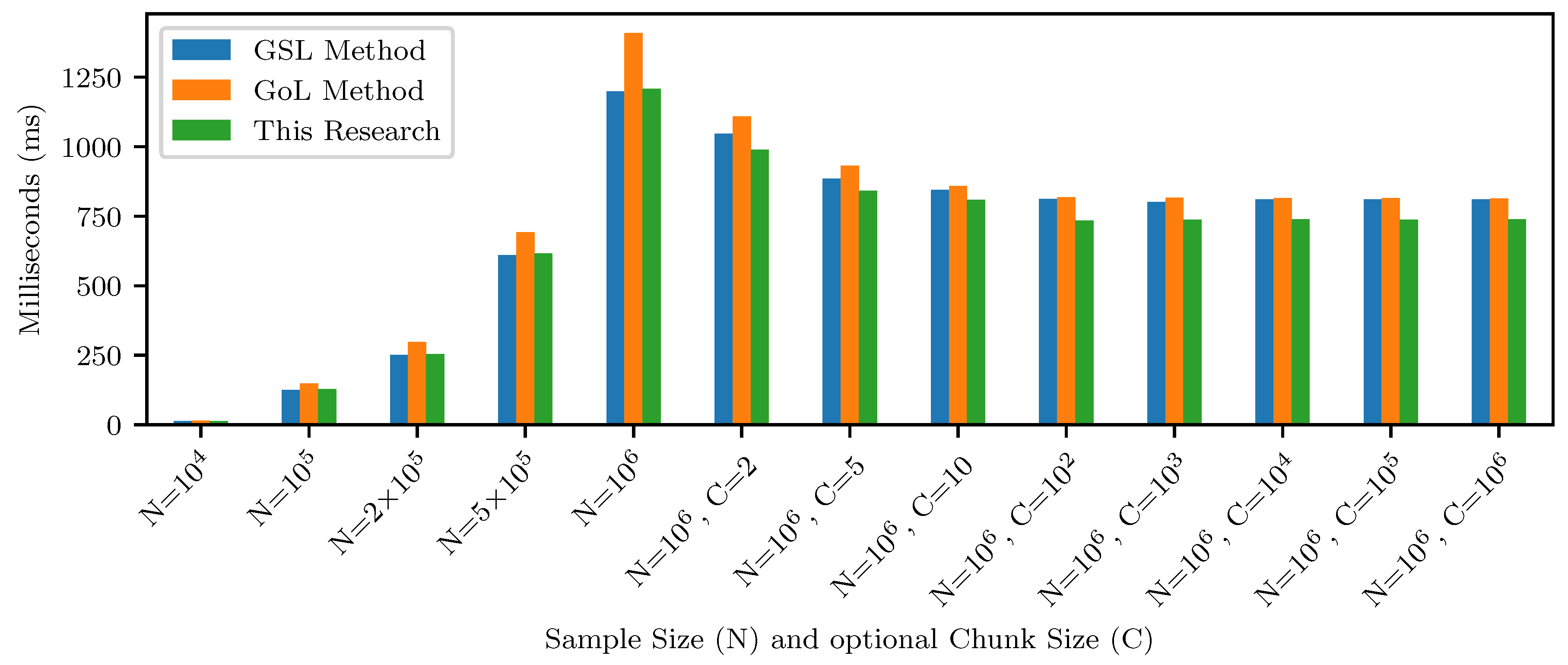
  • The first workload type is to process data one by one. In this research, the programs screen the sample dataset and return the updated CCS value right after every single new price record is included in the processing.
  • The second workload type is to process data chunk by chunk. In this research, the programs return the updated CSS value after every a new price records are included in the processing, while skipping the skewness calculation within the update intervals (i.e., supplementing n % a = = 0 to the if statement in all the algorithms). Note that the intermediate variables outside the if-else block are still updated continuously when screening the sample dataset.

4.3.2. Experimental Results

Inspired by the principle of repeated measures design [47] and by the suggestion of the minimum observation amount [48], we ran the programs ten or more times at each experimental setting. At last, we obtained the three programs’ average running times with respect to different workloads, as exemplified and illustrated in Figure 1.
In general, the running time increases along with the size of the first-type workloads (from N = 10 4 to N = 10 6 ). As for the second-type workloads (from N = 10 6 , C  = 2 to N = 10 6 , C = 10 6 ), it is not surprising that the running time keeps decreasing when skipping more and more skewness calculations. Nevertheless, skipping skewness calculations will have little impact on the running time if the update interval is larger than 100 price records. The reason is the diminishing marginal returns from the reduced workloads. Given the predefined sample size N = 10 6 , when the sample skewness is updated after every 100+ price records, the code within the if-else block will be executed less than 10 4 times. Our extensive experiments have shown that on our testbed, the program execution at such a workload level is so fast that the corresponding running time would be negligible.
Specifically, when dealing with the first-type workloads, the method from this research is slightly slower than the GSL method (about 10 ms on average in our tests), while it is clearly faster than the GoL method (almost 200 ms at the workload size N = 10 6 ). When dealing with the second type of workloads, this research shows a clear advantage over both the GSL method and the GoL method. By using the metric speedup to measure the performance difference, our method can be more than 10% times faster than the other two methods in this case, as demonstrated in Figure 1.
It should be noted that in addition to fitting in the chunk-by-chunk scenario [15], the second workload type is also practical and meaningful when practitioners only need to monitor some samples of CSS values. In practice, the three algorithms can conveniently be modified to update CSS only when receiving request signals. As such, in the case of data-intensive skewness monitoring, we can obtain significant performance enhancement even by halving the update frequency (i.e., updating CSS after every two data records). For example, by switching the workload from N = 10 6 to N = 10 6 , C = 2 (cf. Figure 1), the GSL method and the GoL method receive about 15% and 27% performance improvements, respectively, while our method sees more than 22% performance improvement.

4.3.3. Correctness Verification

Driven by the discussions in [8,9], we decided to use modern software systems of statistics to empirically validate the correctness of our method. For our convenience, we employ Microsoft Excel’s native function SKEW() to return different data samples’ skewness as reference, to verify and compare the calculation results from the GSL method, the GoL method, and our method. In particular, we choose the top N prices records (ranging from the first three records to the first one million records) as data samples from the aforementioned benchmark dataset. The selected validation results are listed in Table 2.
By referring to the output from Microsoft Excel, we claim that both our method and the GoL method can accurately calculate CSS. In contrast, the GSL method delivers different sample skewness values, although the difference becomes smaller and smaller as the sample size grows. This further confirms that due to the employment of Fisher–Pearson skewness coefficient, the GSL method may not be suitable for modern applications. More importantly, considering that online learning only uses a small set of data for its initial training, the big error of skewness from the GSL method may lead to a huge threat to the implementations of skewness-aware online edge learning. Thus, from the perspective of correctness, we suggest avoiding the GSL method when implementing skewness monitoring in production. Note that we have double-confirmed the GSL method’s calculation results by running a C program that directly utilizes the relevant libraries.

4.3.4. Performance Analysis

In addition to the correctness, we analyse the root causes of the performance difference in the three methods by investigating their algorithms together with the experimental results. First, we discuss the reason why the GSL method has the fastest speed when dealing with one-by-one data. Considering that GSL employs the Fisher–Pearson coefficient of skewness whereas GoL and this research employ the adjusted Fisher–Pearson coefficient (cf. Appendix A.3), both the GoL method and our method have involved adjustment overhead in the CSS calculations. However, as mentioned in Section 4.3.3, the de facto software packages/products generally include an adjustment for sample size [8], and thus the GSL method may not be suitable for modern applications.
Then, we discuss the reason why our method has the fastest speed when coping with chunk-by-chunk data. Due to the benefit of the unified pseudo code, it is convenient to count that Algorithm 3 has fewer math operations outside the if-else block than the other two algorithms. Although the operation difference is as small as one multiplication only, the performance difference will be magnified due to large sample sizes, especially in the long-term data streaming scenario. Since there is no need to obtain skewness values within a data chunk (i.e., the code inside the if-else block is not executed in this case), the aforementioned adjustment overhead will be tangibly reduced even if the chunk size is two, which eventually makes our method faster than the GSL method.
As for the GoL method, in addition to the overhead of adjustment and extra multiplication, Algorithm 2 also suffers an avoidable performance loss inside its if-else block. It should be noted that the math operations here can further be simplified into the same form as our method. The current form of Algorithm 2 will be reasonable if the variance value and the skewness value are both needed. However, as shown in Algorithms 1 and 3, the explicit variance calculation is not required when monitoring skewness values only.
Overall, the performance advantage of this research is particularly meaningful and valuable in the context of online edge learning, because practitioners “strive for millisecond-level learning; everything else comes second” [49]. Moreover, considering that IoT devices generally have limited computing and memory capabilities, minimizing operations will be more IoT-friendly and be able to bring significant marginal utility. Even in the broader context of edge cloud computing, any (even small) performance improvement will matter, as “every drop of 20 ms …latency will result in a 7–15% decrease in page load times” [50].

5. Validation and Discussion about Skewness-Aware Online Edge Learning

According to the existing studies on skewness-aware machine learning, the typical strategies of dealing with skewed data include: (1) collecting a suitable number of observations to build a balanced training dataset [5,19], (2) using log transformation to normalise the distribution [19], (3) removing the skewed features when training models [33], (4) employing a penalty function to reduce the impact of skewness [7], etc. Benefiting from the running skewness methods developed in this research, we argue that practitioners will be able to adapt (at least some of) these strategies to different scenarios of online edge learning. As described in the following subsections, we conducted an experimental investigation and proposed a theoretical mechanism to justify the feasibility and usefulness of being aware of skewness in online edge learning.

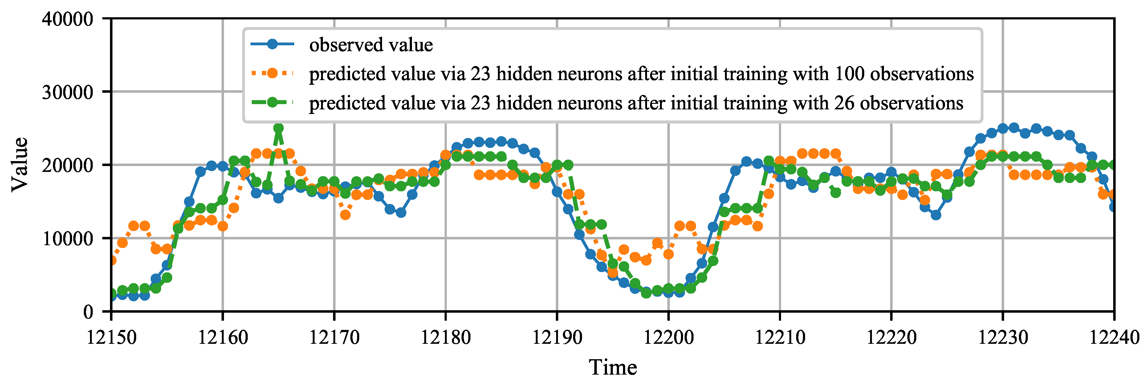
5.1. Automatic Decision Making in Sample Size for Initial Training

Before making predictions at runtime, online learning needs to accumulate a certain number of training data to obtain the first version of model. The de facto strategy seems to use a random or an experience-based size of samples for initial training. For example, the study [14] initializes online learning models using the first 100 observations by default, or using a manually input number of observations. (The variable numLags at https://github.com/chickenbestlover/Online-Recurrent-Extreme-Learning-Machine/blob/master/run.py, accessed on 10 August 2021).
Inspired by the aforementioned first strategy of dealing with skewed data, we propose employing CSS to monitor the skewness of accumulated samples against a predefined threshold, so as to decide the initial training dataset automatically. For ease of comparison, we directly reused the online learning implementations in [14] and slightly modified the source code into a skewness-aware version. Firstly, we commented out the code of standardising the whole dataset, because the online learning “model does not know how many data will be presented” [26]. Secondly, we supplemented Algorithm 3 to the original source code for real-time monitoring of skewness. In particular, since the reported datasets are generally balanced (cf. Section 5.2), we define the skewness threshold to be 0.05 after taking the absolute value.
When the online-sequential extreme learning machine (OS_ELM) over the New York City taxi passenger dataset (i.e., nyc_taxi.csv) is used as an example, the time-series prediction results from executing the original program and our skewness-aware version are both plotted in Figure 2. It should be noted that we kept the default neural network setting (i.e., 100 input neurons, 23 hidden neurons, and 1 output neuron) in this test. In general, every single neuron in a neural network will receive a group of weighted inputs and then return an output after applying an activation function. Given this typical three-layer architecture of the default setting, the input-layer neurons represent individual attributes of the dataset to be learned, the hidden-layer neurons are equipped with non-linear activation functions to be able to solve non-linear problems, and the output-layer neurons can eventually deliver an output that represents the neural network’s prediction.
Compared with the original implementation that uses 100 observations (with skewness value −0.5589) in the initial training, our skewness-aware program automatically selects the first 26 observations (with skewness value −0.0157) to train the initial model. According to the plot shown in Figure 2, intuitively, using fewer training data does not seem to make negative impact on the predication results. On the contrary, the predicted values from the skewness-aware version even better fit the observed values in many cases, e.g., the time series points from 12,150 to 12,160 and from 12,200 to 12,210.
To compare our skewness-aware model with the original model in an objective way, we decided to assess their prediction accuracy quantitatively. Specifically, we follow the study [14] to employ the normalised root-mean-square error (NRMSE) to measure the difference between the observed values and the predicted values. Without standardising the whole dataset, the NRMSE of the original OS_ELM is about 70.06%, while the skewness-aware OS_ELM has a clearly better forecast accuracy at a lower NRMSE value 53.88%.
We further tested different neural network sizes by gradually increasing the number of hidden neurons. The skewness-aware OS_ELM seems always to have an advantage over the original OS_ELM implementation, as listed in Table 3, although the advantage may become trivial with large neural networks. This finding reveals that given a better-trained initial model, the following online learning work can have a higher prediction accuracy, which also makes common sense that “the slightest difference leads to a huge error”.

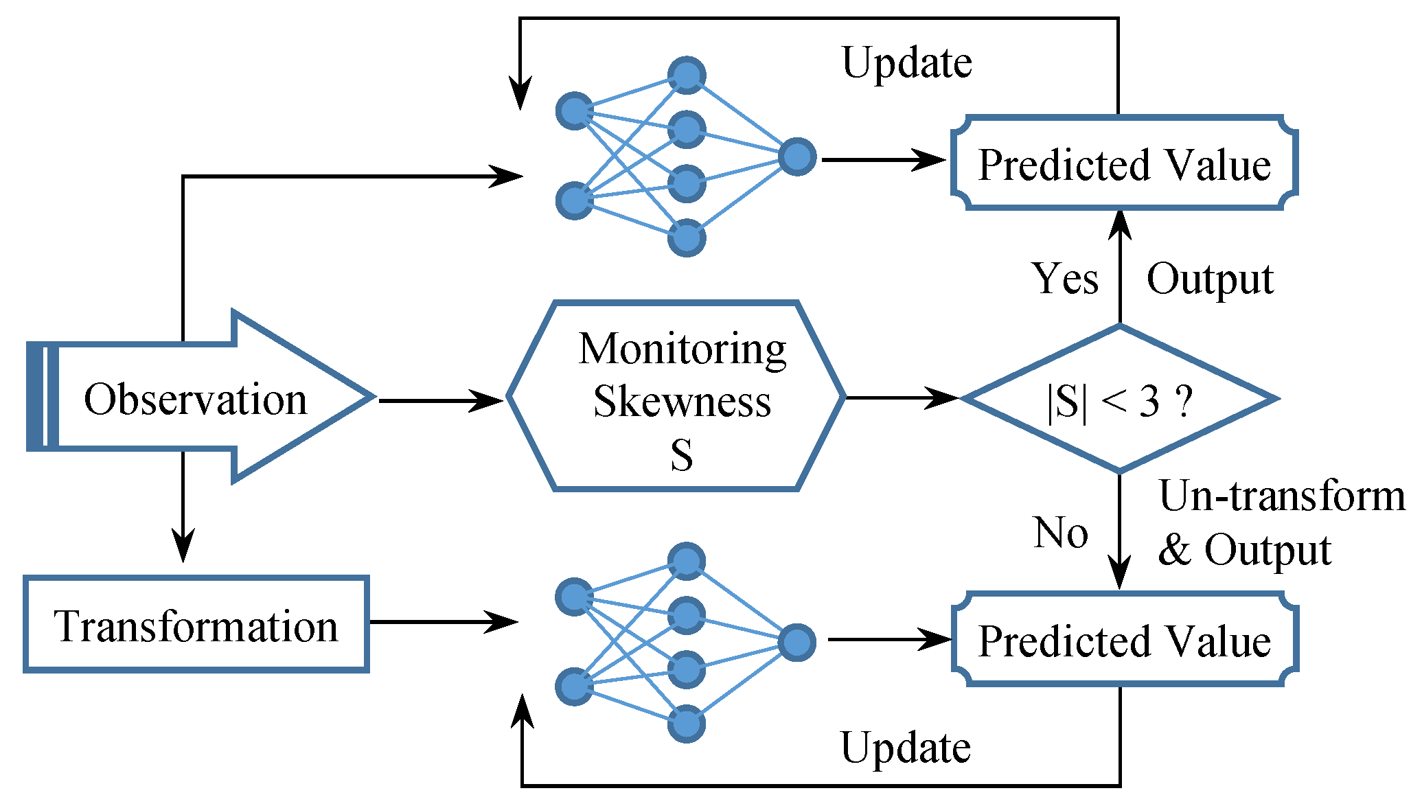
5.2. A Redundancy Mechanism for Skewness-Aware Online Edge Learning

When it comes to the skewness awareness after the initial training stage, inspired by using log transformation to deal with high skewness, we propose maintaining two online learning models respectively over the observed data and over the transformed data at runtime. As such, given a predefined threshold, the online learning system can keep monitoring skewness and accordingly switch between the two models to output predicted values, as illustrated in Figure 3. As for the threshold, according to the suggestions from the literature [51], we distinguish between balanced data and skewed data by checking whether or not the absolute skewness value is less than three.
Such a redundancy mechanism may be particularly suitable for the partially skewed scenario where the online learning logic involves a time/observation window or a forgetting mechanism. Correspondingly, RSS or EWSS can be employed to monitor skewness in this case. It should be noted that this redundancy inevitably requires double computing resources for a single online learning task. Therefore, the cost–benefit analysis should play a prerequisite role in applying the redundancy mechanism to real-world edge environments. In addition, the log transformation can be replaced with other suitable techniques of curing skewed data when implementing this redundancy mechanism.
At the time of writing this paper, we are still exploring suitable (partially skewed) time series data to validate the proposed redundancy mechanism. As discussed in Section 2, it seems that few skewed time series are employed and shared in the community. The lack of reusable skewed data confirms the widely known fact of publication bias, i.e., the existing research may (have to) have intentionally selected balanced datasets to study and publish, because researchers can barely obtain positive results from the online learning techniques over skewed data [6].
Considering the ever-evolving nature of the discipline, we hope to use this proposed redundancy mechanism to inspire more collaboration in skewness-aware online edge learning.

6. Conclusions and Future Work

It is known that machine learning can never do a good job with skewed data. Thus, pre-processing the whole datasets for curing high skewness (e.g., log transformation) has been a common practice before applying machine learning technologies. In edge computing, however, there is no way to conduct such data pre-processing, because it is impractical and impossible to store all the past observations and foresee all the future observations. For the same reason, machine learning at the Internet edge is generally implemented in an online fashion. Correspondingly, it will be valuable to monitor the running skewness of continuous observations before being able to take suitable actions to cure high skewness at runtime.
Nevertheless, when trying to integrate skewness monitoring to online edge learning, we identified a surprising gap between practitioners’ needs and the scientific research in running skewness algorithms. This research bridges the gap by developing a set of IoT-friendly statistical methods to facilitate monitoring skewness at runtime. These methods are essentially based on Welford’s algorithm, which is the most efficient way to calculate running variance. We believe that as an innovation in computer science, Welford’s algorithm might have been overlooked in the statistics community.
More importantly, this research has initially validated the usefulness and significance of being aware of skewness in the implementations of online edge learning. To help boost this promising research field, our future work will unfold along two directions. Firstly, we plan to keep exploring and employing more datasets to strengthen the current validation results. Secondly, we will try to collaborate with more online learning researchers on developing real-time skewness remedies.

Author Contributions

Conceptualization, Z.L. and J.G.-R.; methodology, Z.L.; software, Z.L.; validation, Z.L. and J.G.-R.; formal analysis, Z.L.; investigation, Z.L. and J.G.-R.; resources, Z.L.; data curation, J.G.-R.; writing—original draft preparation, Z.L.; writing—review and editing, Z.L. and J.G.-R.; visualization, Z.L.; funding acquisition, Z.L. Both authors have read and agreed to the published version of the manuscript.

Funding

This research was funded by Chilean National Research and Development Agency (ANID, Chile) under grant FONDECYT Iniciación 11180905.

Institutional Review Board Statement

Not applicable.

Informed Consent Statement

Not applicable.

Data Availability Statement

We reused the New York City taxi passenger dataset (i.e., nyc_taxi.csv) and the implementation of online-sequential extreme learning machine (OS_ELM) algorithm from the open source project at https://github.com/chickenbestlover/Online-Recurrent-Extreme-Learning-Machine, accessed on 10 August 2021.

Acknowledgments

The authors would like to thank Alex Yu who is the owner of GoL (https://github.com/alexander-yu/stream, accessed on 10 August 2021) for his professional help and friendly communication.

Conflicts of Interest

The authors declare no conflict of interest.

Abbreviations

The following abbreviations are used in this manuscript:
CSMCumulative Sample Mean
CSSCumulative Sample Skewness
CSVCumulative Sample Variance
EWSMExponentially Weighted Sample Mean
EWSSExponentially Weighted Sample Skewness
EWSVExponentially Weighted Sample Variance
GNUGNU’s Not Unix
GoLGo-language Library
GPSGlobal Positioning System
GSLGNU Scientific Library
IoTInternet of Things
NRMSENormalised root-mean-square error
OS_ELMOnline-sequential extreme learning machine
RAMRandom-Access Memory
RSMRolling Sample Mean
RSSRolling Sample Skewness
RSVRolling Sample Variance

Appendix A. Opening the Developed Methods

Following the spirit of open methods that act “as a higher-level strategy over open-source tools and open-access data” to facilitate scientific work [20], we also share the proofs of the developed methods in this paper. In fact, the formula derivation details are particularly crucial in the context of running statistics, as discussed in Section 3.1.2.

Appendix A.1. Proof of Equation (2) for Calculating Cumulative Sample Mean (CSM)

Proof. 
Given a series of n observation values x 1 , x 2 , , x n , their arithmetic average x ¯ n can be calculated by Equation (A1):
x ¯ n = i = 1 n x i n
When a new observation value x n + 1 arrives, the sum of the first n values can be substituted by n · x ¯ n for calculating the arithmetic average of the n + 1 values, i.e.,
x ¯ n + 1 = i = 1 n + 1 x i n + 1 = i = 1 n x i + x n + 1 n + 1 = n · x ¯ n + x n + 1 n + 1 = x ¯ n + x n + 1 x ¯ n n + 1
It is clear that x ¯ 0 is zero by default when no value is involved in the average calculation. This completes the proof of Equation (2). □

Appendix A.2. Proof of Equation System (3) for Calculating Cumulative Sample Variance (CSV)

Proof. 
Given a series of n discrete random values x 1 , x 2 , , x n as the sample dataset, the unbiased estimator for the population variance is:
s n 2 = i = 1 n ( x i x ¯ n ) 2 n 1
By introducing the auxiliary notation V , this can be rewritten as:
V n = ( n 1 ) · s n 2 = i = 1 n ( x i x ¯ n ) 2
When a new value x n + 1 arrives, a straightforward modification of the unbiased estimator can be:
V n + 1 = n · s n + 1 2 = i = 1 n + 1 ( x i x ¯ n + 1 ) 2
Then, we calculate the differences between V n + 1 and V n via Equation (A6).
V n + 1 V n = i = 1 n + 1 ( x i x ¯ n + 1 ) 2 i = 1 n ( x i x ¯ n ) 2 = ( x n + 1 x ¯ n + 1 ) 2 + i = 1 n [ ( x i x ¯ n + 1 ) 2 ( x i x ¯ n ) 2 ] = ( x n + 1 x ¯ n + 1 ) 2 + i = 1 n ( 2 x i x ¯ n + 1 x ¯ n ) ( x ¯ n x ¯ n + 1 ) = ( x n + 1 x ¯ n + 1 ) 2 + ( x ¯ n x ¯ n + 1 ) i = 1 n ( 2 x i x ¯ n + 1 x ¯ n )
Recall that i = 1 n x i = n · x ¯ n ; we have:
i = 1 n ( 2 x i x ¯ n + 1 x ¯ n ) = 2 i = 1 n x i n · x ¯ n + 1 n · x ¯ n = i = 1 n x i n · x ¯ n + 1 = ( n + 1 ) · x ¯ n + 1 x n + 1 n · x ¯ n + 1 = x ¯ n + 1 x n + 1
Eventually,
V n + 1 V n = ( x n + 1 x ¯ n + 1 ) 2 + ( x ¯ n x ¯ n + 1 ) ( x ¯ n + 1 x n + 1 ) = ( x n + 1 x ¯ n + 1 ) ( x n + 1 x ¯ n + 1 x ¯ n + x ¯ n + 1 ) = ( x n + 1 x ¯ n + 1 ) ( x n + 1 x ¯ n )
i.e.,
V n + 1 = V n + ( x n + 1 x ¯ n + 1 ) ( x n + 1 x ¯ n )
The sample standard deviation can conveniently be obtained by taking the square root of the unbiased estimator s n + 1 2 . In addition, x ¯ 0 and s 0 2 are initialised as zero by default when no value is involved in the calculation. This completes the proof of Equation System (3). □

Appendix A.3. Proof of Equation System (4) for Calculating Cumulative Sample Skewness (CSS)

Proof. 
Given a series of n observation values x 1 , x 2 , , x n , the symmetry of their distribution is measured by the sample skewness S n :
S n = n ( n 1 ) ( n 2 ) · i = 1 n ( x i x ¯ n ) 3 s n 3
By introducing the auxiliary notation S , this can be rewritten into:
S n = ( n 1 ) ( n 2 ) n · s n 3 · S n = i = 1 n ( x i x ¯ n ) 3
When the dataset includes a new value x n + 1 , we have:
S n + 1 = n ( n 1 ) n + 1 · s n + 1 3 · S n + 1 = i = 1 n + 1 ( x i x ¯ n + 1 ) 3 = i = 1 n ( x i x ¯ n + 1 ) 3 + ( x n + 1 x ¯ n + 1 ) 3
By focusing on i = 1 n ( x i x ¯ n + 1 ) 3 only,
i = 1 n ( x i x ¯ n + 1 ) 3 = i = 1 n [ ( x i x ¯ n ) ( x ¯ n + 1 x ¯ n ) ] 3 = i = 1 n [ ( x i x ¯ n ) 3 3 · ( x i x ¯ n ) 2 ( x ¯ n + 1 x ¯ n ) + 3 · ( x i x ¯ n ) ( x ¯ n + 1 x ¯ n ) 2 ( x ¯ n + 1 x ¯ n ) 3 ] = i = 1 n ( x i x ¯ n ) 3 3 · ( x ¯ n + 1 x ¯ n ) i = 1 n ( x i x ¯ n ) 2 + 3 · ( x ¯ n + 1 x ¯ n ) 2 ( i = 1 n x i n · x ¯ n ) n · ( x ¯ n + 1 x ¯ n ) 3 = i = 1 n ( x i x ¯ n ) 3 3 · ( x ¯ n + 1 x ¯ n ) i = 1 n ( x i x ¯ n ) 2 ( n · x ¯ n + 1 n · x ¯ n ) ( x ¯ n + 1 x ¯ n ) 2 = i = 1 n ( x i x ¯ n ) 3 3 · ( x ¯ n + 1 x ¯ n ) i = 1 n ( x i x ¯ n ) 2 [ n · x ¯ n + 1 ( n + 1 ) · x ¯ n + 1 + x n + 1 ] ( x ¯ n + 1 x ¯ n ) 2 = S n 3 · ( x ¯ n + 1 x ¯ n ) · V n ( x n + 1 x ¯ n + 1 ) ( x ¯ n + 1 x ¯ n ) 2
Thus,
S n + 1 = S n 3 · ( x ¯ n + 1 x ¯ n ) · V n ( x n + 1 x ¯ n + 1 ) ( x ¯ n + 1 x ¯ n ) 2 + ( x n + 1 x ¯ n + 1 ) 3 = S n 3 · ( x ¯ n + 1 x ¯ n ) · V n + ( x n + 1 x ¯ n + 1 ) [ ( x n + 1 x ¯ n + 1 ) 2 ( x ¯ n + 1 x ¯ n ) 2 ] = S n 3 · ( x ¯ n + 1 x ¯ n ) · V n + ( x n + 1 x ¯ n + 1 ) ( x n + 1 x ¯ n ) ( x n + 1 2 x ¯ n + 1 + x ¯ n ) = S n 3 · ( x ¯ n + 1 x ¯ n ) · V n + ( V n + 1 V n ) [ x n + 1 x ¯ n + 1 ( x ¯ n + 1 x ¯ n ) ]
In particular, x ¯ 0 , s 0 , and S 0 are all initialized as zero by default when no observation is involved in the calculation. This completes the proof of Equation System (4). □

Appendix A.4. Proof of Equation (5) for Calculating Rolling Sample Mean (RSM)

Proof. 
Given n observations, the arithmetic average x ¯ n k of the most recent k values is:
x ¯ n k = i = n k + 1 n x i k
After observing a new value x n + 1 , the sample mean within the same size of rolling window can be updated as x ¯ n + 1 k in a recursive manner.
x ¯ n + 1 k = i = n k + 2 n + 1 x i k = i = n k + 1 n x i + x n + 1 x o k = k · x ¯ n k + x n + 1 x o k = x ¯ n k + x n + 1 x o k
In practice, the sample mean x ¯ k k of the first k values should be initialized before rolling the observation window, and thus the total amount of observations n must be at least equal to k and the rolling window size k should not be zero. This completes the proof of Equation (5). □

Appendix A.5. Proof of Equation System (6) for Calculating Rolling Sample Variance (RSV)

Proof. 
Given n observations, the sample variance s n k 2 of the most recent k values is:
s n k 2 = i = n k + 1 n ( x i x ¯ n k ) 2 k 1
By using the notation V to simplify the representation, we rewrite this equation into:
V n k = ( k 1 ) · s n k 2 = i = n k + 1 n ( x i x ¯ n k ) 2
After observing a new value x n + 1 , the k-item sample variance should be updated as:
V n + 1 k = ( k 1 ) · s n + 1 k 2 = i = n k + 2 n + 1 ( x i x ¯ n + 1 k ) 2
Following the same strategy as in Appendix A.2, we calculate the differences between V n + 1 k and V n k via Equation (A20).
V n + 1 k V n k = i = n k + 2 n + 1 ( x i x ¯ n + 1 k ) 2 i = n k + 1 n ( x i x ¯ n k ) 2 = ( x n + 1 x ¯ n + 1 k ) 2 ( x o x ¯ n + 1 k ) 2 + i = n k + 1 n [ ( x i x ¯ n + 1 k ) 2 ( x i x ¯ n k ) 2 ] = ( x n + 1 + x o 2 x ¯ n + 1 k ) ( x n + 1 x o ) + ( x ¯ n k x ¯ n + 1 k ) i = n k + 1 n ( 2 x i x ¯ n k x ¯ n + 1 k )
In particular,
i = n k + 1 n ( 2 x i x ¯ n k x ¯ n + 1 k ) = 2 i = n k + 1 n x i k · x ¯ n k k · x ¯ n + 1 k = 2 k · x ¯ n k k · x ¯ n k k · x ¯ n + 1 k = k · ( x ¯ n k x ¯ n + 1 k ) = x o x n + 1
Thus,
V n + 1 k V n k = ( x n + 1 + x o 2 x ¯ n + 1 k ) ( x n + 1 x o ) + ( x ¯ n k x ¯ n + 1 k ) ( x o x n + 1 ) = ( x n + 1 x o ) ( x n + 1 + x o x ¯ n + 1 k x ¯ n k )
Similarly, the sample variance s k k 2 of the first k values should be initialised before rolling the observation window, and thus the total number of observations n must be at least equal to k, while the rolling window k must be bigger than 1 to avoid the error of division by zero. This completes the proof of Equation System (6). □

Appendix A.6. Proof of Equation System (7) for Calculating Rolling Sample Skewness (RSS)

Proof. 
Given n observations, the sample skewness S n k of the most recent k values is:
S n k = k ( k 1 ) ( k 2 ) · i = n k + 1 n ( x i x ¯ n k ) 3 s n k 3
By using the notation S to simplify the representation, we rewrite Equation (A23) into:
S n k = ( k 1 ) ( k 2 ) · s n k 3 · S n k k = i = n k + 1 n ( x i x ¯ n k ) 3
After observing a new value x n + 1 , Equation (A24) can be updated as:
S n + 1 k = i = n k + 2 n + 1 ( x i x ¯ n + 1 k ) 3 = i = n k + 1 n ( x i x ¯ n + 1 k ) 3 + ( x n + 1 x ¯ n + 1 k ) 3 ( x o x ¯ n + 1 k ) 3
Following the same strategy as in Appendix A.3, we can firstly focus on i = n k + 1 n ( x i x ¯ n + 1 k ) 3 .
i = n k + 1 n ( x i x ¯ n + 1 k ) 3 = i = n k + 1 n [ ( x i x ¯ n k ) ( x ¯ n + 1 k x ¯ n k ) ] 3 = i = n k + 1 n [ ( x i x ¯ n k ) 3 3 ( x i x ¯ n k ) 2 ( x ¯ n + 1 k x ¯ n k ) 3 ( x i x ¯ n k ) ( x ¯ n + 1 k x ¯ n k ) 2 ( x ¯ n + 1 k x ¯ n k ) 3 ] = i = n k + 1 n ( x i x ¯ n k ) 3 k · ( x ¯ n + 1 k x ¯ n k ) 3 3 ( x ¯ n + 1 k x ¯ n k ) i = n k + 1 n ( x i x ¯ n k ) 2 = S n k 3 ( x ¯ n + 1 k x ¯ n k ) · V n k ( k · x ¯ n + 1 k k · x ¯ n k ) ( x ¯ n + 1 k x ¯ n k ) 2 = S n k 3 ( x ¯ n + 1 k x ¯ n k ) · V n k ( x n + 1 x o ) ( x ¯ n + 1 k x ¯ n k ) 2
On the other hand,
( x n + 1 x ¯ n + 1 k ) 3 ( x o x ¯ n + 1 k ) 3 = ( x n + 1 x o ) [ ( x n + 1 x ¯ n + 1 k ) 2 + ( x n + 1 x ¯ n + 1 k ) ( x o x ¯ n + 1 k ) + ( x o x ¯ n + 1 k ) 2 ] = ( x n + 1 x o ) [ ( x n + 1 x ¯ n + 1 k ) ( x n + 1 + x o 2 x ¯ n + 1 k ) + ( x o x ¯ n + 1 k ) 2 ]
Then,
S n + 1 k = S n k 3 ( x ¯ n + 1 k x ¯ n k ) · V n k + ( x n + 1 x o ) [ ( x n + 1 x ¯ n + 1 k ) ( x n + 1 + x o 2 x ¯ n + 1 k ) + ( x o x ¯ n + 1 k ) 2 ( x ¯ n + 1 k x ¯ n k ) 2 ] = S n k 3 ( x ¯ n + 1 k x ¯ n k ) · V n k + ( x n + 1 x o ) [ ( x n + 1 x ¯ n + 1 k ) ( x n + 1 + x o 2 x ¯ n + 1 k ) + ( x o x ¯ n k ) ( x o 2 x ¯ n + 1 k + x ¯ n k ) ]
To initialise the sample skewness S k k 2 of the first k values before rolling the observation window, the total number of observations n must be at least equal to k, while the rolling window k must be bigger than two to avoid the error of division by zero. This completes the proof of Equation System (7). □

Appendix A.7. Proof of Equation (8) for Calculating Exponentially Weighted Sample Mean (EWSM)

Proof. 
We refer to [36] to briefly rephrase the derivation of the EWSM formula. Similarly, the derivation starts from the discussion about CSM by rewriting (2) as:
x ¯ n + 1 = x ¯ n + x n + 1 x ¯ n n + 1 = n n + 1 · x ¯ n + 1 n + 1 · x n + 1
It is clear that when the observation amount n approaches infinity, the new observation value x n + 1 will barely play a part in the calculation of the sample mean, which violates the EWSM scenario where the more recent data are more valuable/significant. In contrast, by replacing the item 1 n + 1 with a constant coefficient α between 0 and 1, and correspondingly replacing n n + 1 with ( 1 α ) , the contribution of older observations will become progressively smaller. Eventually, we obtain the equation for calculating EWSM as follows.
x ¯ w ( n + 1 ) = ( 1 α ) · x ¯ w ( n ) + α · x n + 1
In particular, to avoid confusion with the notation x ¯ n , we use x ¯ w ( n ) to denote the sample mean that involves all the existing weighting effects. Moreover, in this form, a bigger α discounts older data faster. This completes the proof of Equation (8). □

Appendix A.8. Proof of Equation (9) for Calculating Exponentially Weighted Sample Variance (EWSV)

Proof. 
Following the same strategy of drawing the EWSM formula, we start the derivation from rewriting the CSV formula (3) into:
n · s n + 1 2 = ( n 1 ) · s n 2 + ( x n + 1 x ¯ n + 1 ) ( x n + 1 x ¯ n )
and then:
s n + 1 2 = ( 1 1 n ) · s n 2 + 1 n · ( x n + 1 x ¯ n + 1 ) ( x n + 1 x ¯ n )
There is no doubt that increasing observation amount n will decrease the contribution of new value x n + 1 to the variance calculation. By fixing a constant coefficient β between 0 and 1 to replace 1 n , we obtain Equation (A33) for calculating EWSV:
s w ( n + 1 ) 2 = ( 1 β ) · s w ( n ) 2 + β · ( x n + 1 x ¯ w ( n + 1 ) ) ( x n + 1 x ¯ w ( n ) )
We use the notation s w ( n ) 2 to indicate the sample variance that involves the past weighting effects. Similar to α , a bigger β also discounts older data faster in this case. This completes the proof of Equation (9). □

Appendix A.9. Proof of Equation System (10) for Calculating Exponentially Weighted Sample Skewness (EWSS)

Proof. 
Given the previous proofs for EWSM and EWSV, a natural deduction is that the EWSS formula can be obtained from the CSS formula by replacing its n-related parameters with suitable constant coefficients. Therefore, we can rewrite Equation System (4) as:
n · ( n 1 ) n + 1 · s n + 1 3 · S n + 1 = ( n 1 ) ( n 2 ) n · s n 3 · S n 3 · ( x ¯ n + 1 x ¯ n ) ( n 1 ) · s n 2 + ( x n + 1 x ¯ n + 1 ) ( x n + 1 x ¯ n ) [ x n + 1 x ¯ n + 1 ( x ¯ n + 1 x ¯ n ) ]
and then:
n 1 n + 1 · s n + 1 3 · S n + 1 = ( 1 2 n + 1 ) · s n + 1 3 · S n + 1 = ( 1 1 n ) ( 1 2 n ) · s n 3 · S n 3 · ( x ¯ n + 1 x ¯ n ) ( 1 1 n ) · s n 2 + 1 n · ( x n + 1 x ¯ n + 1 ) ( x n + 1 x ¯ n ) [ x n + 1 x ¯ n + 1 ( x ¯ n + 1 x ¯ n ) ]
By reusing the predefined constant coefficients, i.e., replacing 1 n + 1 and 1 n with α and β respectively, we have:
( 1 2 α ) · s w ( n + 1 ) 3 · S w ( n + 1 ) = ( 1 β ) ( 1 2 β ) · s w ( n ) 3 · S w ( n ) 3 · ( x ¯ w ( n + 1 ) x ¯ w ( n ) ) ( 1 β ) · s w ( n ) 2 + β · ( x n + 1 x ¯ w ( n + 1 ) ) ( x n + 1 x ¯ w ( n ) ) · [ x n + 1 x ¯ w ( n + 1 ) ( x ¯ w ( n + 1 ) x ¯ w ( n ) ) ]
where S w ( n ) differs from S n and denotes the sample skewness that involves the past weighting effects. As regulated previously, the constant coefficients α and β are two decimal numbers between 0 and 1. Since both of them are used in the EWSS formula, for the purpose of consistence, we further regulate their relationship as follows through the replaced items.
1 α 1 β = 1
This completes the proof of Equation System (10). □

References

  1. Chen, D.; Liu, Y.C.; Kim, B.; Xie, J.; Hong, C.S.; Han, Z. Edge Computing Resources Reservation in Vehicular Networks: A Meta-Learning Approach. IEEE Trans. Veh. Technol. 2020, 69, 5634–5646. [Google Scholar] [CrossRef]
  2. Gómez-Carmona, O.; Casado-Mansilla, D.; Kraemer, F.A.; de Ipiña, D.L.; García-Zubia, J. Exploring the computational cost of machine learning at the edge for human-centric Internet of Things. Future Gener. Comput. Syst. 2020, 112, 670–683. [Google Scholar] [CrossRef]
  3. Li, X.; Han, Q.; Qiu, B. A clustering algorithm using skewness-based boundary detection. Neurocomputing 2018, 275, 618–626. [Google Scholar] [CrossRef]
  4. Radečić, D. Top 3 Methods for Handling Skewed Data. 2020. Available online: https://towardsdatascience.com/top-3-methods-for-handling-skewed-data-1334e0debf45 (accessed on 17 January 2021).
  5. Zhang, L.; Tang, K.; Yao, X. Log-normality and skewness of estimated state/action values in reinforcement learning. In Proceedings of the 31st International Conference on Neural Information Processing Systems (NIPS 2017); ACM Press: Long Beach, CA, USA, 2017; pp. 1802–1812. [Google Scholar]
  6. Vasudev, R. How to Deal with Skewed Dataset in Machine Learning? 2017. Available online: https://becominghuman.ai/how-to-deal-with-skewed-dataset-in-machine-learning-afd2928011cc (accessed on 17 January 2021).
  7. Sun, Y.; Todorovic, S.; Li, J. Reducing the Overfitting of AdaBoost by Controlling its Data Distribution Skewness. Int. J. Pattern Recognit. Artif. Intell. 2006, 20, 1093–1116. [Google Scholar] [CrossRef] [Green Version]
  8. Doane, D.P.; Seward, L.E. Measuring Skewness: A Forgotten Statistic? J. Stat. Educ. 2011, 19, 1–18. [Google Scholar] [CrossRef]
  9. Macroption. Skewness Formula. 2021. Available online: https://www.macroption.com/skewness-formula/ (accessed on 17 January 2021).
  10. Lombardi, M.; Pascale, F.; Santaniello, D. Internet of Things: A General Overview between Architectures, Protocols and Applications. Information 2021, 12, 87. [Google Scholar] [CrossRef]
  11. Merenda, M.; Porcaro, C.; Iero, D. Edge Machine Learning for AI-Enabled IoT Devices: A Review. Sensors 2020, 20, 2533. [Google Scholar] [CrossRef]
  12. Tuor, T.; Wang, S.; Salonidis, T.; Ko, B.J.; Leung, K.K. Demo Abstract: Distributed Machine Learning at Resource-Limited Edge Nodes. In Proceedings of the 2018 IEEE Conference on Computer Communications Poster and Demo (INFOCOM’18 Poster/Demo), Honolulu, HI, USA, 15–19 April 2018; pp. 1–2. [Google Scholar]
  13. GNU. Running Statistics. 2019. Available online: https://www.gnu.org/software/gsl/doc/html/rstat.html (accessed on 12 January 2021).
  14. Park, J.M.; Kim, J.H. Online recurrent extreme learning machine and its application to time-series prediction. In Proceedings of the 2017 International Joint Conference on Neural Networks (IJCNN 2017), Anchorage, AK, USA, 14–19 May 2017; pp. 1983–1990. [Google Scholar]
  15. Liang, N.Y.; Huang, G.B.; Saratchandran, P.; Sundararajan, N. A Fast and Accurate Online Sequential Learning Algorithm for Feedforward Networks. IEEE Trans. Neural Netw. 2006, 17, 1411–1423. [Google Scholar] [CrossRef]
  16. MathWorks. Moving Skewness and Moving Kurtosis. 2018. Available online: https://www.mathworks.com/matlabcentral/answers/426189-moving-skewness-and-moving-kurtosis (accessed on 12 January 2021).
  17. StackExchange. Exponential Weighted Moving Skewness/Kurtosis. 2011. Available online: https://stats.stackexchange.com/questions/6874/exponential-weighted-moving-skewness-kurtosis (accessed on 12 January 2021).
  18. StackOverflow. Is There Any Built in Function in Numpy to Take Moving Skewness? 2019. Available online: https://stackoverflow.com/questions/57097809/is-there-any-built-in-function-in-numpy-to-take-moving-skewness (accessed on 19 January 2021).
  19. Choi, J.H.; Kim, J.; Won, J.; Min, O. Modelling Chlorophyll-a Concentration using Deep Neural Networks considering Extreme Data Imbalance and Skewness. In Proceedings of the 21st International Conference on Advanced Communication Technology (ICACT 2019), PyeongChang, Korea, 17–20 February 2019; pp. 631–634. [Google Scholar]
  20. Li, Z.; Li, X.; Li, B. In Method We Trust: Towards an Open Method Kit for Characterizing Spot Cloud Service Pricing. In Proceedings of the 12th IEEE International Conference on Cloud Computing (CLOUD 2019), Milan, Italy, 8–13 July 2019; pp. 470–474. [Google Scholar]
  21. Jin, H.; Jia, L.; Zhou, Z. Boosting Edge Intelligence With Collaborative Cross-Edge Analytics. IEEE Internet Things J. 2021, 8, 2444–2458. [Google Scholar] [CrossRef]
  22. Abelson, H.; Ledeen, K.; Lewis, H.; Seltzer, W. Blown to Bits: Your Life, Liberty, and Happiness after the Digital Explosion, 2nd ed.; Addison-Wesley Professional: Boston, MA, USA, 2020. [Google Scholar]
  23. Zhu, G.; Liu, D.; Du, Y.; You, C.; Zhang, J.; Huang, K. Toward an Intelligent Edge: Wireless Communication Meets Machine Learning. IEEE Commun. Mag. 2020, 58, 19–25. [Google Scholar] [CrossRef] [Green Version]
  24. Wang, S.; Tuor, T.; Salonidis, T.; Leung, K.K.; Makaya, C.; He, T.; Chan, K. When Edge Meets Learning: Adaptive Control for Resource-Constrained Distributed Machine Learning. In Proceedings of the 37th IEEE Conference on Computer Communications (INFOCOM 2018), Honolulu, HI, USA, 16–19 April 2018; pp. 63–71. [Google Scholar]
  25. Yazici, M.T.; Basurra, S.; Gaber, M.M. Edge Machine Learning: Enabling Smart Internet of Things Applications. Big Data Cogn. Comput. 2018, 2, 26. [Google Scholar] [CrossRef] [Green Version]
  26. Li, G.; Liu, M.; Dong, M. A new online learning algorithm for structure-adjustable extreme learning machine. Comput. Math. Appl. 2010, 60, 377–389. [Google Scholar] [CrossRef] [Green Version]
  27. Aral, A.; Erol-Kantarci, M.; Brandić, I. Staleness Control for Edge Data Analytics. Proc. ACM Meas. Anal. Comput. Syst. 2020, 4, 38. [Google Scholar] [CrossRef]
  28. Huang, Z.; Lin, K.J.; Tsai, B.L.; Yan, S.; Shih, C.S. Building edge intelligence for online activity recognition in service-oriented IoT systems. Future Gener. Comput. Syst. 2018, 87, 557–567. [Google Scholar] [CrossRef]
  29. Kadirkamanathan, V.; Niranjan, M. A Function Estimation Approach to Sequential Learning with Neural Networks. Neural Comput. 1993, 5, 954–975. [Google Scholar] [CrossRef]
  30. Li, Y.; Wang, X.; Gan, X.; Jin, H.; Fu, L.; Wang, X. Learning-Aided Computation Offloading for Trusted Collaborative Mobile Edge Computing. IEEE Trans. Mob. Comput. 2020, 19, 2833–2849. [Google Scholar] [CrossRef]
  31. Qi, K.; Yang, C. Popularity Prediction with Federated Learning for Proactive Caching at Wireless Edge. In Proceedings of the 2020 IEEE Wireless Communications and Networking Conference (WCNC 2020), Seoul, Korea, 25–28 May 2020; pp. 1–6. [Google Scholar]
  32. Scardapane, S.; Comminiello, D.; Scarpiniti, M.; Uncini, A. Online Sequential Extreme Learning Machine With Kernels. IEEE Trans. Neural Netw. Learn. Syst. 2015, 26, 2214–2220. [Google Scholar] [CrossRef]
  33. Shahadat, N.; Pal, B. An empirical analysis of attribute skewness over class imbalance on Probabilistic Neural Network and Naïve Bayes classifier. In Proceedings of the 1st International Conference on Computer and Information Engineering (ICCIE 2015), Rajshahi, Bangladesh, 26–27 November 2015; pp. 150–153. [Google Scholar]
  34. Pham, M.T.; Cham, T.J. Online Learning Asymmetric Boosted Classifiers for Object Detection. In Proceedings of the 2007 IEEE Conference on Computer Vision and Pattern Recognition (CVPR 2007), Minneapolis, MN, USA, 17–22 June 2007; pp. 1–8. [Google Scholar]
  35. Zhao, J.; Wang, Z.; Park, D.S. Online sequential extreme learning machine with forgetting mechanism. Neurocomputing 2012, 87, 79–89. [Google Scholar] [CrossRef]
  36. Tham, M.T. Exponentially Weighted Moving Average Filter. 2009. Available online: https://web.archive.org/web/20091212013537/http://lorien.ncl.ac.uk/ming/filter/filewma.htm (accessed on 17 January 2021).
  37. Serel, D.A.; Moskowitz, H. Joint economic design of EWMA control charts for mean and variance. Eur. J. Oper. Res. 2008, 184, 157–168. [Google Scholar] [CrossRef] [Green Version]
  38. Knuth, D.E. Art of Computer Programming, Volume 2: Seminumerical Algorithms, 3rd ed.; Addison-Wesley Professional: Boston, MA, USA, 1997. [Google Scholar]
  39. Cook, J.D. Accurately Computing Running Variance. Available online: https://www.johndcook.com/blog/standard_deviation/ (accessed on 17 January 2021).
  40. StackExchange. Recursive Formula for Variance. 2013. Available online: https://math.stackexchange.com/questions/374881/recursive-formula-for-variance (accessed on 12 January 2021).
  41. Teknomo, K. Proof Recursive Variance Formula. 2006. Available online: https://people.revoledu.com/kardi/tutorial/RecursiveStatistic/ProofTime-Variance.htm (accessed on 12 January 2021).
  42. Weisstein, E.W. Sample Variance Computation. From MathWorld—A Wolfram Web Resource. Available online: https://mathworld.wolfram.com/SampleVarianceComputation.html (accessed on 12 January 2021).
  43. StackOverflow. Rolling Variance Algorithm. 2018. Available online: https://stackoverflow.com/questions/5147378/rolling-variance-algorithm (accessed on 19 January 2021).
  44. Taylor, M. Running Variance. 2010. Available online: http://www.taylortree.com/2010/11/running-variance.html (accessed on 19 January 2021).
  45. Pébay, P.; Terriberry, T.B.; Kolla, H.; Bennett, J. Numerically stable, scalable formulas for parallel and online computation of higher-order multivariate central moments with arbitrary weights. Comput. Stat. 2016, 31, 1305–1325. [Google Scholar] [CrossRef] [Green Version]
  46. Li, Z.; O’Brien, L.; Kihl, M. DoKnowMe: Towards a Domain Knowledge-driven Methodology for Performance Evaluation. ACM SIGMETRICS Perform. Eval. Rev. 2016, 43, 23–32. [Google Scholar] [CrossRef] [Green Version]
  47. Montgomery, D.C. Design and Analysis of Experiments, 9th ed.; John Wiley & Sons, Inc.: Hoboken, NJ, USA, 2019. [Google Scholar]
  48. Jenkins, D.G.; Quintana-Ascencio, P.F. A solution to minimum sample size for regressions. PLoS ONE 2020, 15, e0229345. [Google Scholar] [CrossRef] [PubMed] [Green Version]
  49. Pagels, M. What Is Online Machine Learning? 2018. Available online: https://medium.com/value-stream-design/online-machine-learning-515556ff72c5 (accessed on 27 February 2021).
  50. Strom, D.; van der Zwet, J.F. Truth and Lies about Latency in the Cloud. White Paper, Interxion. 2021. Available online: https://www.interxion.com/whitepapers/truth-and-lies-of-latency-in-the-cloud/download (accessed on 19 July 2021).
  51. Chen, K.C.; Jang, S.J. Motivation in online learning: Testing a model of self-determination theory. Comput. Hum. Behav. 2010, 26, 741–752. [Google Scholar] [CrossRef]
Figure 1. CSS algorithm performance comparison among the GSL method, the GoL method, and this research’s method with respect to different workloads.
Applsci 11 07461 g001
Figure 2. Time-series prediction of the online-sequential extreme learning machine (OS_ELM) over the nyc_taxi dataset.
Applsci 11 07461 g002
Figure 3. The redundancy mechanism for skewness-aware online edge learning.
Applsci 11 07461 g003
Table 1. Notations used in the rest of this paper.
NotationExplanation
nAmount of observations (samples) within a time series.
n k The most recent k items from a time series of n samples, and n k > 0 .
s n Sample standard deviation of n observation values x 1 , x 2 , , x n .
s n 2 Sample variance of n observation values x 1 , x 2 , , x n .
s n k 2 Sample variance of the most recent k out of n observation values x n k + 1 , x n k + 2 , , x n .
s w ( n ) 2 Exponentially weighted sample variance of a time series of n observation values.
S n Sample skewness of n observation values x 1 , x 2 , , x n .
S n k Sample skewness of the most recent k out of n observation values x n k + 1 , x n k + 2 , , x n .
S w ( n ) Exponentially weighted sample skewness of a time series of n observation values.
x i The ith observation value within a time series, and i > 0 .
x o Value of the oldest observation within the most recent k out of n observation values.
x ¯ n Sample mean of a time series of n observation values x 1 , x 2 , , x n .
x ¯ n k Sample mean of the most recent k out of n observation values x n k + 1 , x n k + 2 , , x n .
x ¯ w ( n ) Sample mean of a time series of n observation values x 1 , x 2 , , x n with exponentially decreasing weights.
α , β constant coefficients between 0 and 1 for discounting the contribution of older data.
S n Auxiliary variable that carries the crucial information of the third Central Moment.
S n k Auxiliary variable that is associated with, and is to update, S n k .
V n Auxiliary variable that carries the crucial information of the second Central Moment.
V n k Auxiliary variable that is associated with, and is to update, s n k 2 .
C 2 , C 3 Auxiliary variables (similar to V n and S n ) that are used in the Go Library.
M 2 , M 3 Auxiliary variables (similar to V n and S n ) that are used in GNU Scientific Library.
Table 2. Three Methods’ CSS Calculation Results against EXCEL Output.
Sample SizeGSL MethodGoL MethodThis ResearchExcel Skew( )
3−0.378753−1.704387−1.704387−1.704387
4−0.749576−1.998869−1.998869−1.998869
5−0.292042−0.608421−0.608421−0.608421
10−0.944882−1.312336−1.312336−1.312336
1004.5936224.7347174.7347174.734717
10006.0751316.0933996.0933996.093399
10,0005.8821055.8838705.8838705.883870
100,00044.20090544.20223244.20223244.202232
1,000,00043.52873843.52886943.52886943.528869
Table 3. Prediction Accuracy Comparison between Original OS_ELM and Skewness-aware OS_ELM.
Number of Hidden NeuronsOriginal OS_ELMSkewness-Aware OS_ELM
23NRMSE:  70.06%NRMSE:  53.88%
50NRMSE:  50.85%NRMSE:  48.14%
100NRMSE:  41.41%NRMSE:  38.77%
200NRMSE:  36.33%NRMSE:  33.11%
Publisher’s Note: MDPI stays neutral with regard to jurisdictional claims in published maps and institutional affiliations.

