Article

CAD/CAM System for Additive Manufacturing with a Robust and Efficient Topology Optimization Algorithm Based on the Function Representation

Center for Design, Manufacturing and Materials, Skolkovo Institute of Science and Technology, 30/1 Bolshoi Boulevard, 121205 Moscow, Russia
*
Author to whom correspondence should be addressed.
Appl. Sci. 2021, 11(16), 7409; https://doi.org/10.3390/app11167409
Submission received: 20 July 2021 / Revised: 6 August 2021 / Accepted: 9 August 2021 / Published: 12 August 2021
(This article belongs to the Section Mechanical Engineering)

Abstract

:
Additive manufacturing erases the distance between design ideas and finished parts. However, designers must use several software tools to use these advantages. Moreover, these tools operate with different representations of geometry. This paper describes the architecture of a new CAD/CAM system that uses only the function representation of the geometry (FRep). It provides all widely used design operations and allows an engineer to employ robust and efficient topology optimization algorithms. The developed CAD/CAM system consists of 3D modeling, simulation, topology optimization, and direct manufacturing modules. We successfully printed designed parts and performed mechanical tests of printed parts. The results of tests show good agreement with simulation data. The system makes it possible to create structures with the desired properties in a fast and flexible way. The proposed approach significantly helps in designing additive manufacturing process and saves time for its users.

1. Introduction

The design stage in the manufacturing process has become more complex in recent decades [1]. Designers try to create details that fully correspond to their intended functionality. This translates into certain mass limits and stiffness requirements to designed parts. Simulation and topology optimization algorithms help obtain the geometry satisfying these constraints. However, topology optimization algorithms can produce geometries that are impossible with traditional production methods but suitable for additive manufacturing (AM) [2]. These technologies impose new requirements to computer-aided design (CAD) and computer-aided manufacturing (CAM) software. Moreover, they significantly increase the complexity of CAD models that can be manufactured, and clearly show the limitations of boundary representation (BRep) used in traditional CAD/CAM systems. Application of multiple settheoretic and other operations, varying the parameters of BRep models, leads to corruption of meshes and significantly increases the size of files with resulting geometry for models in high precision applications [3]. The use of BRep leads to occurrence of incorrect faces in exported STL files or errors in the slicing process. Moreover, when a design includes the analysis or topology optimization steps, the traditional approach uses the following geometry transformations. First, the BRep CAD geometry is transformed to the voxel representation, and then analysis and topology optimization is performed. Second, the BRep is reconstructed with possible smoothing. Finally, the resulting geometry is sliced to create a computer numerical control (CNC) program in a specific language such as G-code [4]. Several software packages usually serve these purposes.
The use of the FRep-based CAD/CAM system instead resolves all previously mentioned problems of the BRep format. In contrast to BRep, function representation (FRep) guarantees the correctness of resulting geometry regardless of the number of set theoretic and other operations and the number of parameters in the model [5]. The paper [6] presents the fundamentals of the FRep. It supports many modeling operations. The basis of settheoretic operations are R-functions [7]. Operations on FRep objects have become the subject of several studies, including blending, bending, offsetting, sweeping [8], bounded blending, trimming [9], metamorphosis, etc. [10]. The mentioned theory of R-functions was initially developed as a tool for domains modeling in partial differential equations (PDE) [7]. Later publications elaborated this approach [11] and proposed an algorithm for topology optimization of FRep models [12]. Many algorithms employ the FRep for domain description in various simulation and structural optimization tasks [13,14]. These algorithms form a group called level-set methods for topology optimization. The advantage of such optimization algorithms is their ability to directly provide the optimal geometry in contrast to 0–1 density methods such as the solid isotropic material with penalization (SIMP) method [14]. FRep-based optimization algorithms provide ready-to-print shapes in contrast to BRep-based methods requiring post-processing steps, e.g., smoothing the geometry, leading to remodeling of the body. Level-set methods for multi-material topology optimization exist [15]. For example, they can be applied for designing of continuous fiber-reinforced structures instead of existing topology optimization methods [16,17]. Thus, FRep can be applied to solve various tasks; however, no complete FRep-based CAD/CAM system has yet been proposed.
The presented work has two contributions. The first is the aggregation of FRep and level-set methods in one CAD/CAM system. Both FRep and level-set methods operate with continuous functions for describing domains. It allowed us to develop the first framework that provides tools for topology optimization and uses its results as modeling primitives for further design. The second contribution is the modification of the level-set-based topology optimization algorithm. These modifications increased the speed of the algorithm up to 90 times and improved its stability. This paper describes a CAD/CAM system that uses FRep for all modeling, analysis, topology optimization, and direct manufacturing operations. The system was tested by 3D printing of a designed part. The part was obtained by structural optimization of a rectangular domain with the simulation of its mechanical properties. The simulated properties were experimentally validated.

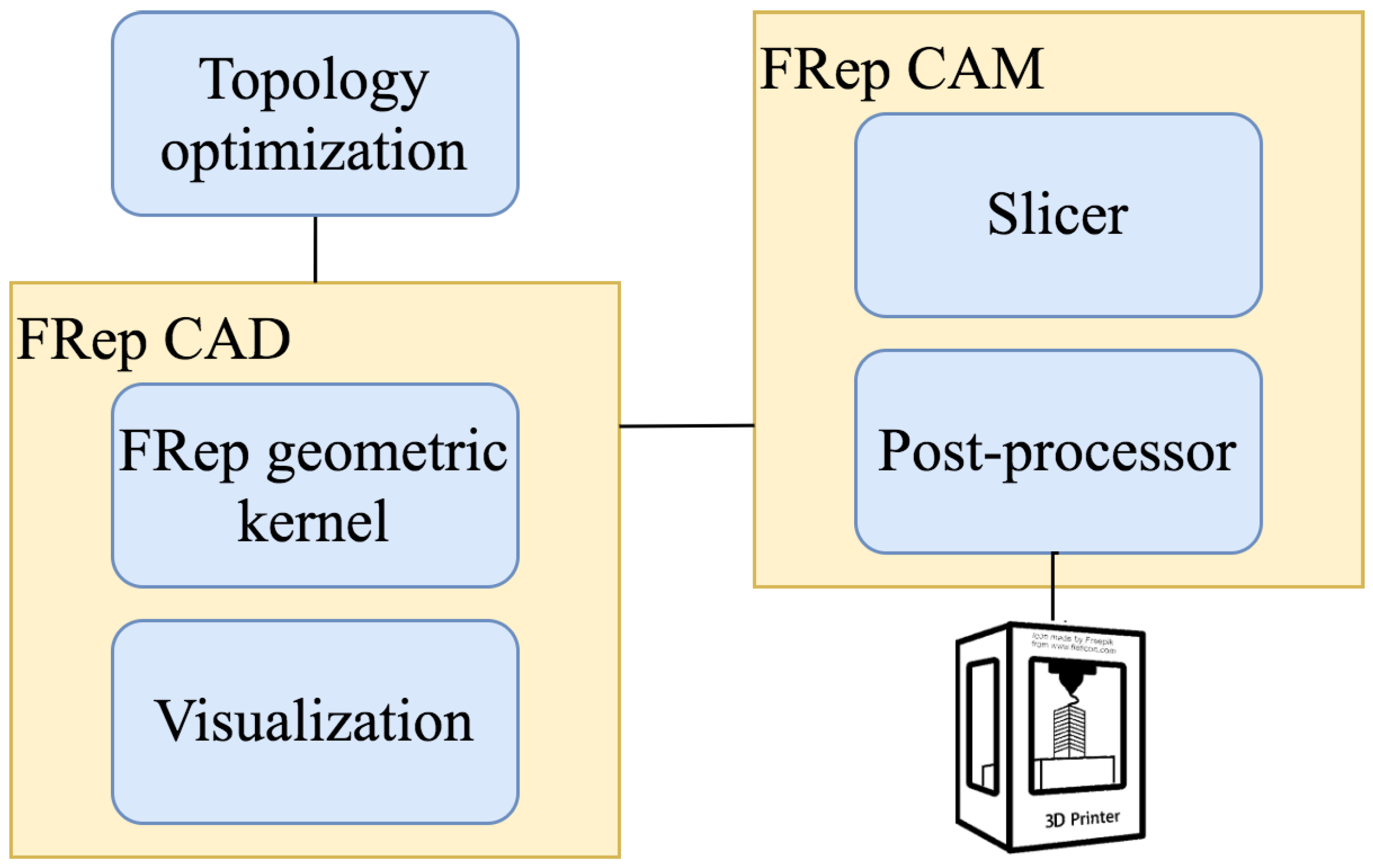
2. Software Structure and Methods

We propose the FRep-based CAD/CAM system that makes it possible to rapidly design and print optimized parts. Figure 1 shows the principal components of the FRep system. The key part of the developed system is an FRep kernel connecting all modules of the system. An FRep defining function sets up the classification rule to obtain boundary segments of the body with the given precision. The FRep kernel supports the import and export of models from other CAD systems. Data from this component are used both in direct manufacturing routines and in visualization. Moreover, the defining function is processed as a level-set function in optimization and analysis algorithms.
The next essential component of the system is the FRep CAM module. This component is responsible for interactions with additive manufacturing equipment. Its main routine is slicing of FRep models. However, this procedure can take hours in high precision applications where the slice thickness is 10,000 times smaller than the size of a model. Techniques described in [18] can speed up the contouring step but they do not work well in the case of models with high porosity and defining functions with loops. The post-processing follows the contouring step. The post-processor generates G-code to control AM equipment [19]. Let us consider all mentioned components of the system in more details.

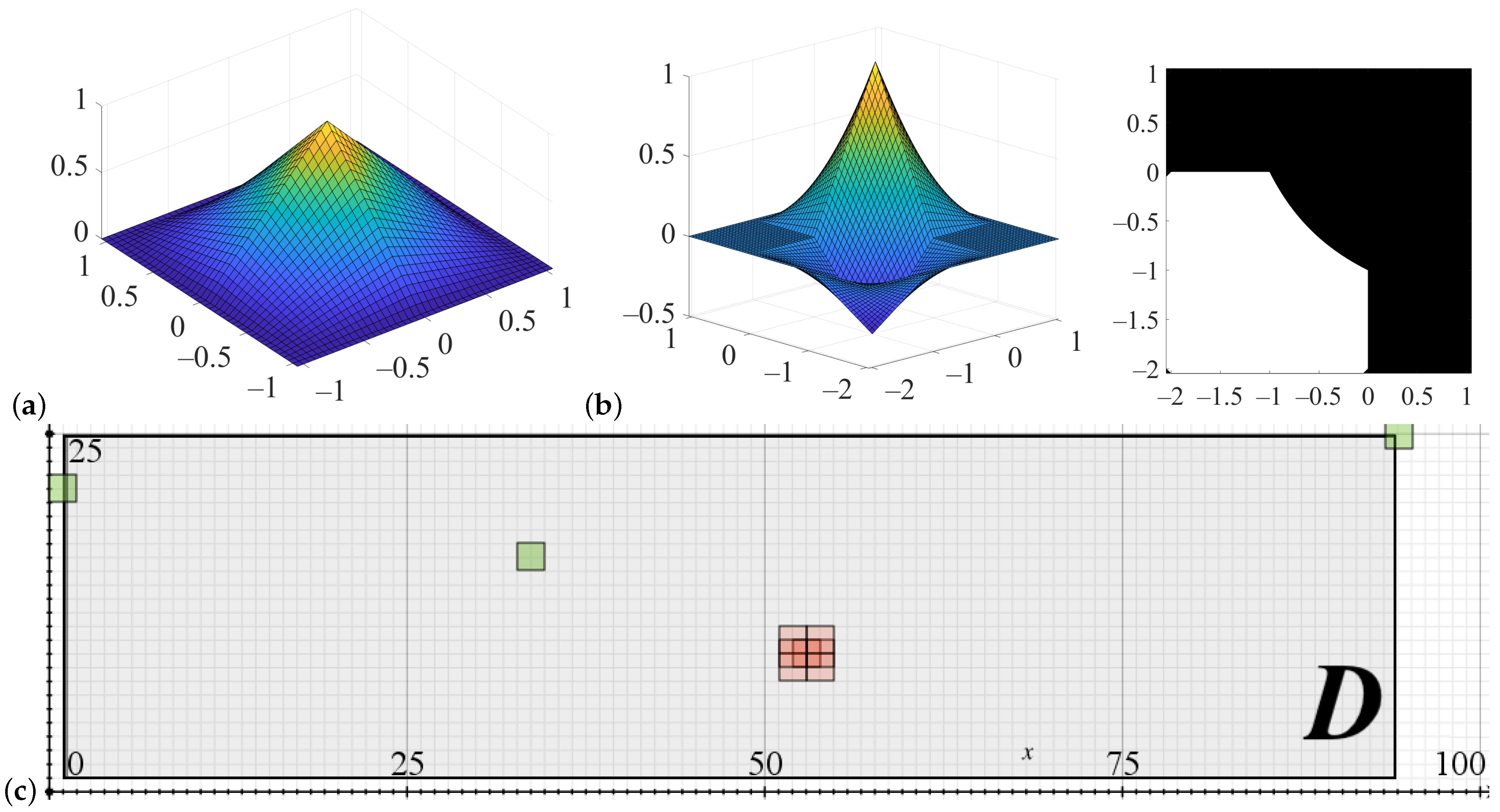
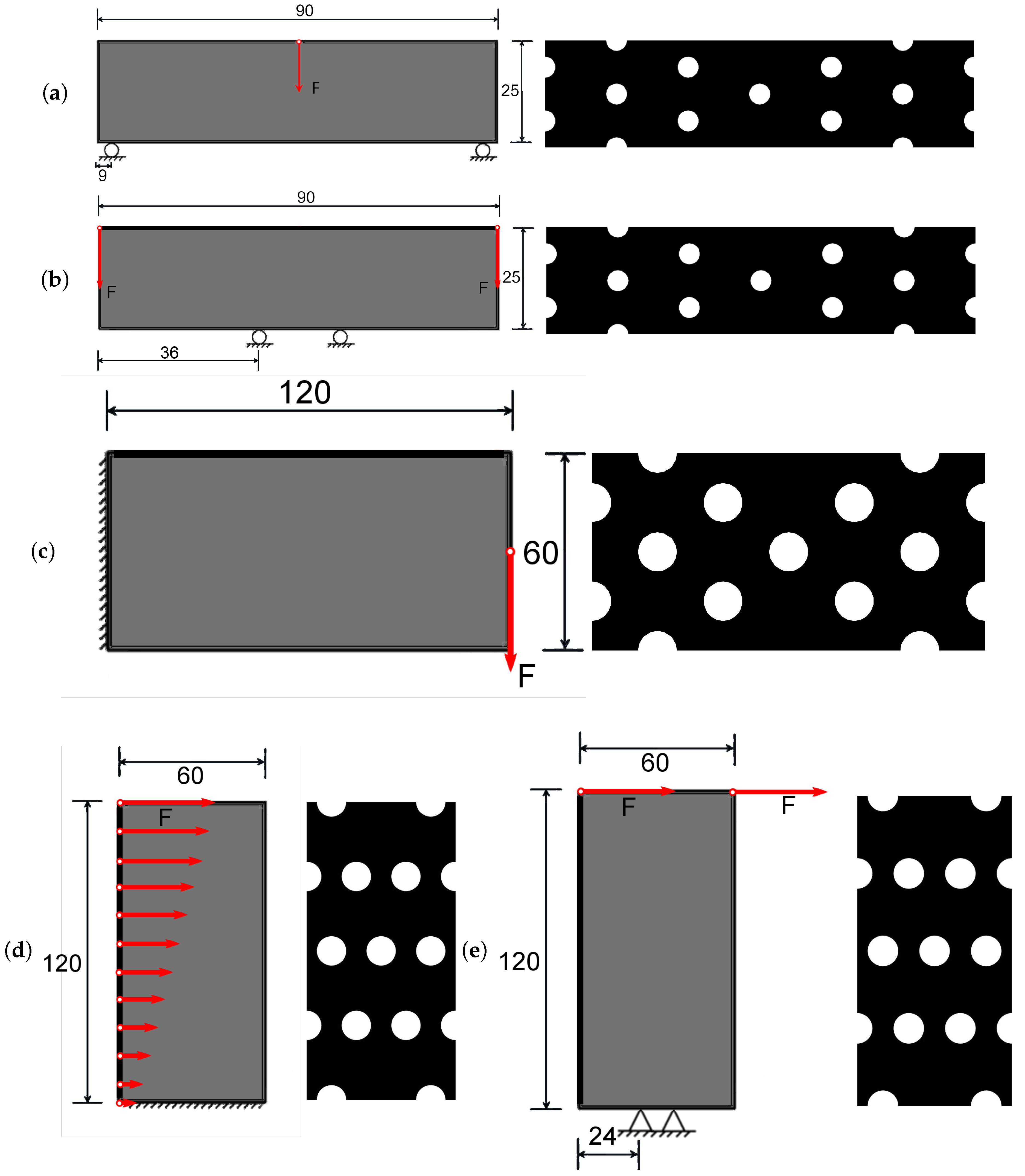
2.1. Topology Optimization

The developed system uses the modified topology optimization algorithm presented in [20]. For the 2D topology optimization case the compliance minimization problem used in the system can be expressed as follows:
minimize(over f) J 0 ( u ) = D E i j k l ε i j ( u ) ε k l ( u ) H ( f ) d Ω ,
subject to: a ( u , v , f ) = l ( v , f ) , v U ,
u | Γ 1 = u 0 ,
E i j k l ε i j ( u ) | Γ 2 = p ,
D H ( f ) d Ω V 0 ,
where
a ( u , v , f ) = D E i j k l ε i j ( u ) ε k l ( v ) H ( f ) d Ω , l ( v , f ) = D g v + ( p v n ) H ( f ) d Ω , H ( f ) = 1 if f 0 , 0 f < 0 ,
J 0 ( u ) is an elastic energy, the objective function; u—the displacement field; ε i j ( u ) and ε k l ( u ) —the linearized strain tensors; E i j k l —the Hook elasticity tensor; u 0 , p and g—the constant values that represent the given displacement, traction and body force respectively; a ( u , v , f ) is the linear elastic equilibrium equation written in its weak, variational form and l ( v , f ) is the load linear form, with v denoting a virtual displacement field in the space U of kinematically admissible displacement fields; V 0 is the maximum allowable volume in the design domain D; H ( f ) is the Heaviside function that represents the presence of material at a point of the level-set function value f:
H ( f ) = 1 if f 0 0 if f < 0
This problem statement uses the level-set function f which, at the same time, is an FRep defining function f ( x 1 , x 2 , . . . , x n ) (see Section 2.2):
f ( x 1 , x 2 , . . . , x n ) > 0 , if ( x 1 , x 2 , . . . , x n ) Ω = 0 , if ( x 1 , x 2 , . . . , x n ) Ω < 0 , if ( x 1 , x 2 , . . . , x n ) Ω ¯
where f is a real continuous function defined on E n , n equals 2 for 2D, and 3 for 3D topology optimization, respectively.
Let us consider the 2D optimization. The proposed topology optimization algorithm incorporates a free-form defining function with bilinear basis functions:
ϕ ( x , y ) = ( 1 | x | ) ( 1 | y | ) if | x | 1 and | y | 1 0 otherwise .
This function defines a surface drawn in Figure 2a. Moreover, in general case, we need to use this equation with constants h 1 and h 2 to define a rectangular non-zero region of the spline basis function, as follows:
ϕ ( x , y ) = ( 1 1 h 1 | x | ) ( 1 1 h 2 | y | ) if | x | h 1 and | y | h 2 0 otherwise
However, the form (4) can be used here without the loss of generality. This form of the spline basis function is well suited for the further discussion. Space mapping is used to locate spline basis function at some portion of the domain. The bilinear spline basis function with the center of the non-zero region at ( x i , y i ) is:
ϕ i ( x , y ) = ( 1 | x x i | ) ( 1 | y y i | ) if | x x i | 1 and | y y i | 1 0 otherwise .
Therefore, the free-form defining function (3) used here can be expressed as follows:
f ( x , y ) = i = 1 N α i ϕ i ( x , y )
with constants α i .
The main steps of the proposed modified algorithm are shown in Algorithm 1.
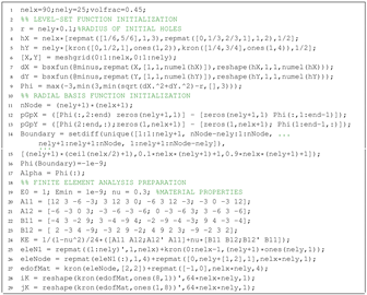
Algorithm 1: The proposed topology optimization algorithm.
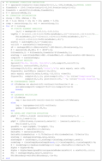
 Step 1. Define the number of grid elements in the rectangular domain n e l x × n e l y ;
 Step 2. Initialize coefficients of the bilinear spline;
 Step 3. Define boundary conditions for FEM analysis;
 Step 4. Initialize parameters of the optimization loop;
 Step 5. Perform FEM analysis of the domain;
 Step 6. If the algorithm converges, then quit, else update α i and go to Step 5.
The following equation is used to update the free-form function (3):
V n = V · ( f | f | ) , f t V n | f | = 0 ,
where t is the pseudo time representing the evolution of the free-form function, and V n is the outward normal velocity chosen based on the shape derivative of the optimization problem. The equation for updating α i is as follows:
α i ( t j + 1 ) = α ¯ i ( t j ) + Δ t Φ 1 B ( α ¯ i ( t j ) , t j ) ,
where
α ¯ i ( t j ) = α i ( t j ) m e a n ( | f ( x 1 1 , x 2 1 , . . . , x n 1 , t j ) | , | f ( x 1 2 , x 2 2 , . . . , x n 2 , t j ) | , . . . , | f ( x 1 r , x 2 r , . . . , x n r , t j ) | , Φ = ϕ 1 ( x 1 1 , x 2 1 , . . . , x n 1 ) ϕ N ( x 1 1 , x 2 1 , . . . , x n 1 ) ϕ 1 ( x 1 N , x 2 N , . . . , x n N ) ϕ N ( x 1 N , x 2 N , . . . , x n N ) ,
( x 1 1 , x 2 1 , . . . , x n 1 ) , . . . , ( x 1 r , x 2 r , . . . , x n r ) are the points near the solid boundary, ( x 1 1 , x 2 1 , . . . , x n 1 ) , . . . , ( x 1 N , x 2 N , . . . , x n N ) are the knot points of the bilinear spline (3), B ( α ¯ i ( t j ) , t j ) is the velocity vector at the time step t j :
B ( α ¯ i ( t j ) , t j ) = V n ( x 1 1 , x 2 1 , . . . , x n 1 , t j ) δ ( f ( x 1 1 , x 2 1 , . . . , x n 1 , α ¯ i ( t j ) ) ) V n ( x 1 N , x 2 N , . . . , x n N , t j ) δ ( f ( x 1 N , x 2 N , . . . , x n N , α ¯ i ( t j ) ) ) .
For the compliance minimization problem (1), the normal velocity V n can be derived as follows:
V n = E i j k l ε i j ( u ) ε k l ( u ) λ
where λ is the Lagrange multiplier to deal with the constraint of the volume fraction, which is calculated using the following augmented Lagrangian updating scheme:
λ k + 1 = μ G k k n R λ k + γ k G k > n R ,
where μ and γ k are parameters in the k-th iteration of the optimization, and γ k is updated using the following scheme:
γ k + 1 = m i n ( γ k + Δ γ , γ m a x ) k > n R .
where Δ γ is the increment and γ m a x is the upper limit of the parameter γ . Since the volume fraction of initial design usually does not meet the prescribed volume fraction, the volume constraint is relaxed in the first n R iterations as below:
G k = D H ( f ) d Ω V 0 ( V 0 V m a x ) k n R k n R .
To avoid the unbounded growth of the free-form function, an approximate δ ( f ) function is inserted into the velocity vector of (11), defined as follows:
δ ( f ) = 0 f < Δ 3 4 ( 1 f 2 Δ 2 ) Δ f Δ 0 f > Δ ,
where the parameter Δ is used to control the magnitude of the upper and lower bounds of the free-form function. The ersatz material model is used in the finite element analysis to obtain the naturally extended velocity field from the strain energy density in the whole design domain. The MATLAB implementation of the proposed optimization algorithm is given in the Appendix A.

2.2. FRep Geometric Kernel
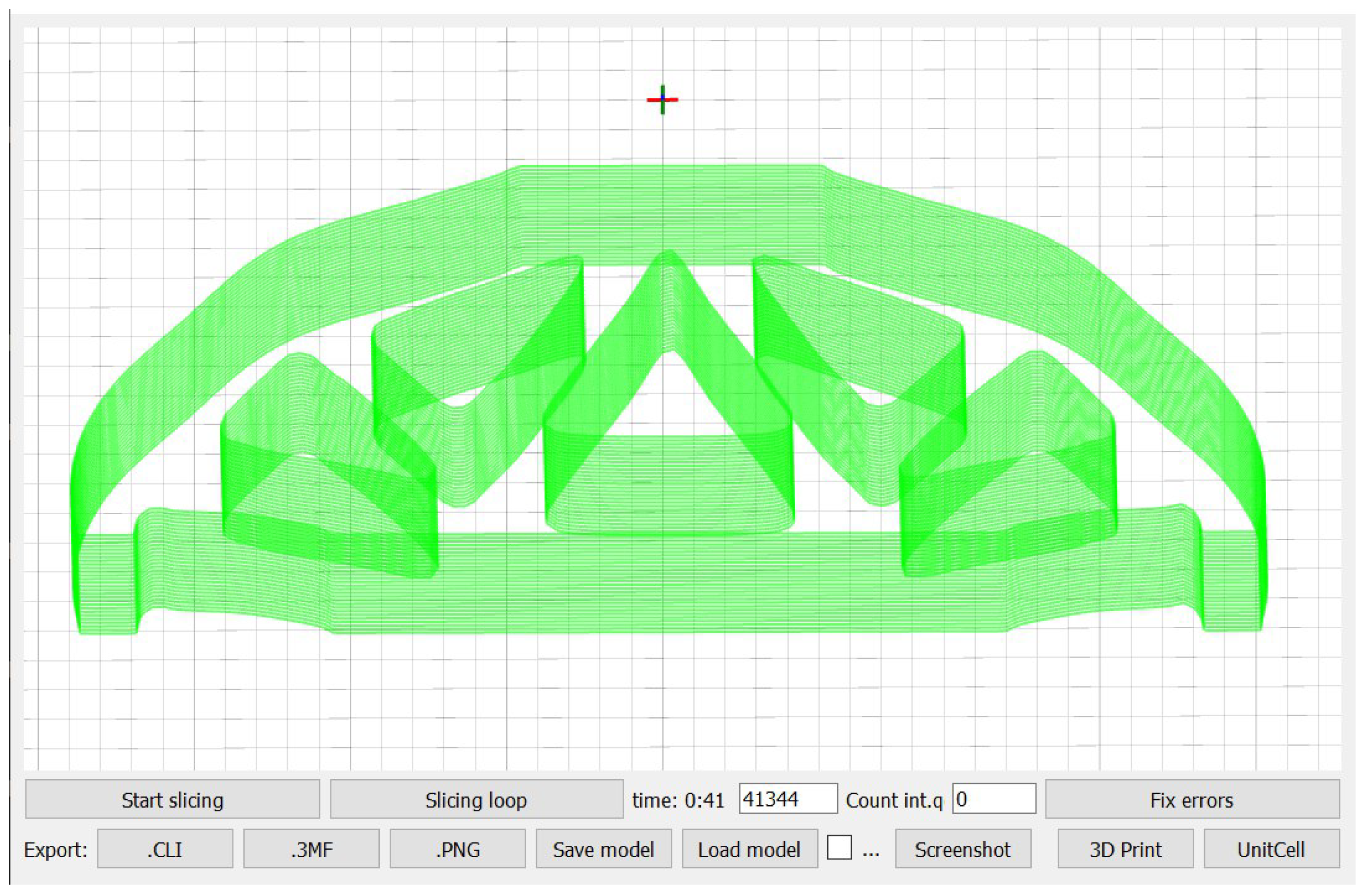
The core concept of an FRep-based geometric kernel is a solid body. Its formal definition is a closed subset of an n-dimensional Euclidean space E n . The defining function (3) describes a solid body in the FRep format. A simple example of defining function is:
f ( x , y ) = 1 R ( R 2 ( x x 0 ) 2 ( y y 0 ) 2 )
which describes a disk in E 2 , with its center in ( x 0 , y 0 ) and radius R.
The FRep geometric kernel allows designers to create complex bodies from primitives as shown in (17), using modeling operations. A constructed complex body complies the classification rule (3) and includes all parameters of used primitives, such as center coordinates ( x 0 , y 0 ) and radius R of a disk primitive (17). The FRep geometric kernel supports R-functions [7] determining set-theoretic operations. Two examples are presented in Figure 3. Moreover, the FRep supports blending, bending, offsetting, sweeping [8], bounded blending, trimming [9], metamorphosis, etc. [10].

2.3. Visualization

The developed system visualizes objects via level contours (see Figure 4) obtained during the slicing procedure. Therefore, contours serve two goals—visualization and direct slicing for G-code generation (see Section 2.4). Although this is not the fastest way to draw a body, this technique allows us to represent printed objects layer by layer. This approach is useful for interactions with 3D printers, as it helps detect possible manufacturing issues, e.g., overhangs.
The system uses the contouring algorithm described in [18]. A user defines an interval of z coordinates and a step size to set up the slice where the system calculates contours. For each value of z, the algorithm computes contours as a sequence of line segments. The length of these segments depends on the required accuracy. We can speed up the contouring process using the interval arithmetic in the marching squares (MS) algorithm [19,21]. To render generated contours, the freeglut [22] library is used.

2.4. Direct Slicing

The concept of direct manufacturing assumes the preparation of a 3D model for fabrication without an intermediate step of surface generation in a special format such as STL. This means that 2D contours for toolpath generation are extracted directly during the slicing process of an FRep object. One of the first mentions of direct manufacturing for AM can be found in [23], and its application for FRep models is described in [19]. Direct manufacturing of the 3D model for 3D printing consists of the following stages:
  • Slicing of the model.
  • Contour extraction (contouring).
  • Generation of the supports and infilling.
  • Generation of the management protocol for the additive manufacturing equipment.
The system supports direct manufacturing for fused filament fabrication (FFF), direct metal deposition (DMD) and digital light processing (DLP) 3D printers. The MS algorithm with the adaptive optimization technique is applied for contour extraction. The open source CuraEngine [24] is used to generate supports and infilling. It allows creation of different infill patterns (see Figure 5) and generation of management protocol (G-code) for FFF and DMD printers. The DLP equipment requires the CWS format. The FRep CAM generates the G-code for print bed control and a set of raster layers to control layer illumination, included in CWS files.

2.5. 3D Printing

Figure 6 (bottom) shows the metal 3D part manufactured according to the geometry shown in Figure 7a, left. It is still attached to the cylindrical substrate with marks of previously printed parts here. The part was printed at a 3D printer TruPrint 1000 (Trumpf) of stainless steel powder (Höganäs AB 316L, Germany). The analysis of the powder is presented in the study [25]. The printing process parameters were chosen according to the manufacturer recommendations. Material parameters, such as Young’s modulus and Poisson’s ratio, were obtained from results of tensile tests performed according to the ASTM E8/E8M procedure [26], using an Instron 5969 testing machine (Instron). The plate samples with gage section of 2.0 × 6.0 mm2 and gage length of 25.0 mm were tested at the loading speed of 10 3 s 1 .

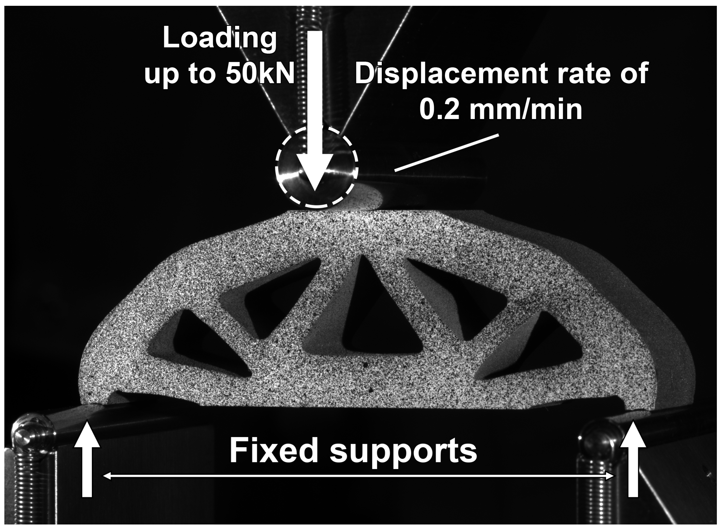
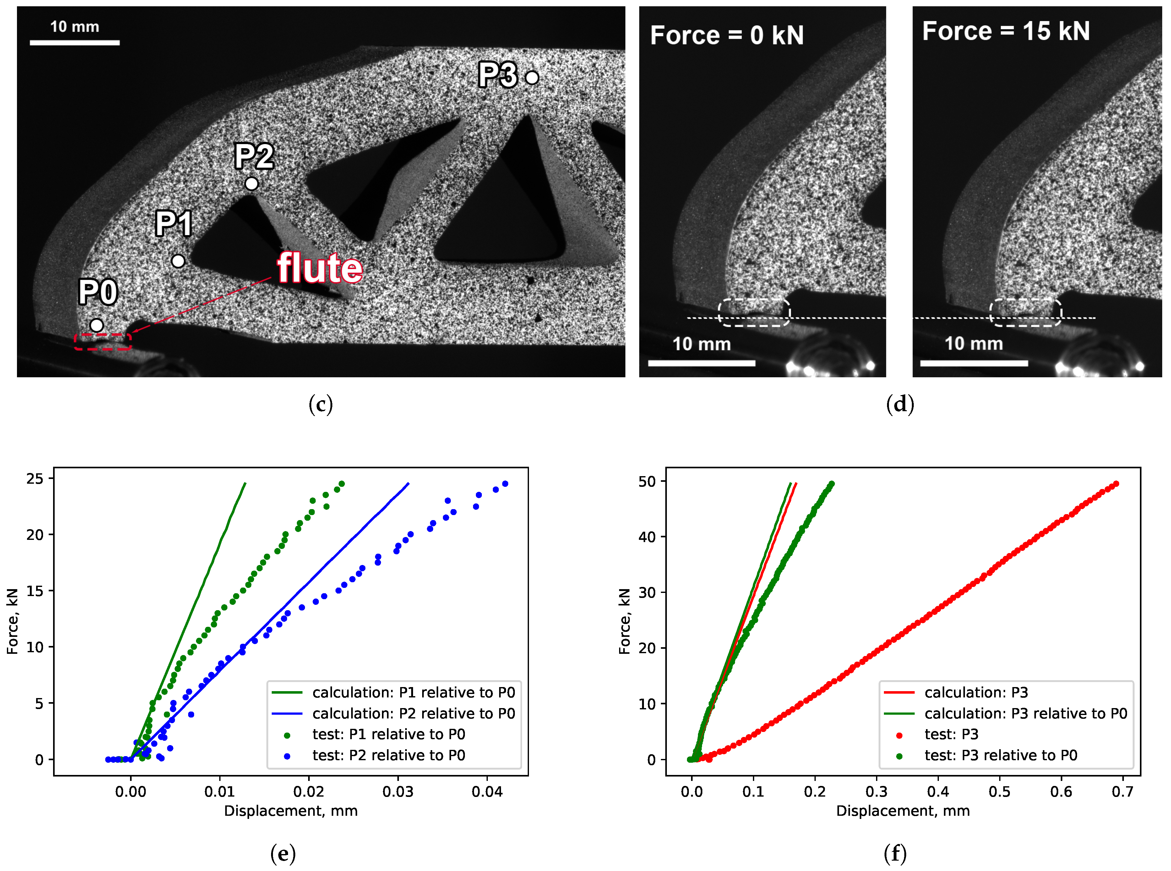
2.6. Experimental Validation

The 3D printed part was tested in the three-point bending mode following the procedure specified in ASTM D790 [27]. An Instron 5969 testing machine equipped with 6.0 mm diameter round supports and a 12.0 mm diameter loading bar for the three-point bending test was used. The tests were conducted with a loading bar displacement rate of 0.2 mm/min, which moved up to a load of 50 kN, according to Figure 8. To measure the strain, we used the Digital Image Correlation System (Correlated Solutions, Irmo, SC, USA) recording the displacement of points during the test. The images were taken at every 100 N load increment. To increase the stability of the part during the test, several flutes were manufactured as shown in Figure 9 (red dotted area).

3. Results and Discussion

3.1. Modifications of the Topology Optimization Algorithm

The free-form function (7) uses bilinear basis functions instead of MultiQuadric (MQ) basis proposed in the original algorithm [20]. The use of bilinear basis functions has several advantages. First, the α i from (7) has a simple interpretation. The only spline basis function placed at some point ( x i , y i ) with positive coefficient α i means that its non-zero region [ x i 1 , x i + 1 ] , [ y i 1 , y i + 1 ] is filled with material. Otherwise, if α i is negative, no material is present in [ x i 1 , x i + 1 ] , [ y i 1 , y i + 1 ] . Two spline basis functions ϕ i ( x , y ) and ϕ j ( x , y ) with shared non-zero regions and corresponding α i and α j of opposite signs define a portion of the body in the shared region with the boundary defined by the equation:
α i ( 1 | x x i | ) ( 1 | y y i | ) = α j ( 1 | x x j | ) ( 1 | y y j | ) .
The Equation (18) defines a conic section in 2D. Figure 2b shows the case of two bilinear spline basis functions with the shared region and corresponding α i and α j of opposite signs. The black region on the right is the domain where the considered function is positive.
Second, the algorithm proposed in [20] works with a rectangular domain D and the bilinear spline (7) can accurately describe it. Consider the domain as shown in Figure 2c covered by 91 × 26 spline basis functions. Three non-zero regions of the bilinear spline basis functions are shown in green, seven shared non-zero regions of the bilinear spline basis functions are shown in red. Grid knots are the centers of their non-zero regions. Every non-zero region of a spline basis function covers four white regions. However, it is not the case for the basis functions placed at the boundary of D. One can define the whole rectangular domain D by a finite number of spline functions in the form proposed in Equation (7).
Two conditions hold for all these functions. The α i values corresponding to all spline basis functions placed at the boundary, equal zero, and others are positive. The optimization algorithm requires the free-form function (7) to have properties of a signed distance function near the boundary. Therefore, for example, for the basis functions placed at the boundary, α i can be initialized with zeros, and in other cases—with unities.
One more reason to use bilinear splines in Equation (3) is the FEM step. At this step, we approximate the Young’s modulus of the rectangular element proportionally to the element’s density. For the elements with no material, the Young’s modulus is assumed to be zero. Young’s modulus of elements filled with material is assumed to be equal to that of proposed material. The algorithm estimates the density of elements partially located at the boundary. It uses exact values of the bilinear spline (7).
Another modification [20] relates to Steps 2 and 6 of the initial optimization algorithm. In the examples from [20], the defining function initially has positive values at the boundary of the domain D. From the FRep perspective, it means that the body has a surface somewhere outside D. However, it is not correct. Mathematically, α i at the boundary of the domain D has to be zero or negative.
Suppose at some iteration i of the algorithm we obtained the defining function f i ( x , y ) . The idea above can be written as:
f i ( x j , y j ) = m i n ( f i 1 ( x j , y j ) , 0 )
where ( x j , y j ) is a boundary point of D.
The rule introduced above has an exception. Consider the boundary conditions for the case shown in Figure 10a, left. The shown body has three special points. There are two points where the body touches rollers and the point where force F is applied. Let us suppose that another body produces this force. Therefore, near these three points, we have a region where we cannot easily separate optimized body and external bodies. These points always contain a portion of material. Thus, Equation (19) does not hold for them.
One implementation issue should be noted (see the MATLAB code in the Appendix A). Consider the initialization of the bilinear spline defining the body shown in Figure 10a, right. It is a meaningful option of the body design, but it has holes at the boundary of D. Small negative values are used in Equation (19) instead of zero to allow the algorithm to go over similar shapes.
This modification of Equation (19) is also useful in one more situation. During the optimization process, at some iteration i, we can obtain the defining function (7) with all positive α j . It is true for all points except ones mentioned in (19). Replacement of zero with some small negative value prevents the algorithm error at the normalization step (10). The above-mentioned modifications make the algorithm more robust.
We compared the proposed modified topology optimization algorithm with the original one [20]. The laptop with the following characteristics was used for tests: Windows 10 Enterprise 64-bit operating system, x64-based processor Intel(R) Core(TM) i5-8250U CPU @ 1.60 GHz 1.80 GHz, and 8.00 GB (7.86 GB usable) of installed memory (RAM). Both algorithms, the original one and the modified one, were run 10 times with following initial datasets. The domain grid is as shown in Figure 2c. The initial geometry is as shown in Figure 10a, right. Boundary conditions are taken from Figure 10a, left (see details in Appendix A). The desired volume, V 0 , was chosen as 45% of the volume of the entire D. The Young’s modulus of stainless steel, E 0 , is assumed to be 205 G P a , and the Poisson’s ratio, ν , is assumed to be 0.27 . Stainless steel is a material obtained of the powder used for 3D printing. The properties of material were studied in [25]. In the original algorithm all parameters of the updating scheme for f i ( x , y ) were preserved, except the time step. The time step was changed to 0.2. These parameters were also used for the modified algorithm.
Both algorithms exploit an isotropic material model at the FEM step. However, the research [25] showed that 3D printed parts have anisotropy. Nevertheless, the validation results (see Section 3.3) showed that the isotropic model of material is suitable for the considered cases.
Results of the computational test are shown in Table 1. We can see that the modified algorithm is approximately twice as fast as the original one. It can be easily explained using different spline basis functions. When the bilinear spine is used instead of the MQ-spline, the time-consuming operation of matrix inversion is not needed. Two obtained optimized bodies are shown in Figure 7a.
Four more optimization cases shown in Figure 10 were considered to check the observed tendency. Figure 7 shows the results of optimization algorithms testing. Efficiency of the algorithms for these cases is compared in Table 2. The results show that the modified algorithm is faster.
The difference in efficiency is much higher for finer grids of basis functions in the domain. The original algorithm became 20 times slower than the modified algorithm at the case shown in Figure 7c, which can be explained by the matrix inversion used in the Wei’s optimization.
At the same time, both algorithms produce similar values of the objective function, differing in the third significant digit, depending on the optimization case.
Small modifications of the algorithm listed in Appendix A were used to produce models shown in Figure 7. These modifications are listed in Appendix A.
As in the case of direct slicing, more accurate optimization takes more time and requires more RAM installed. Both tasks, slicing and optimization, lead to the solution of the trade-off between precision and time. Although calculations on the mentioned laptop provide valid data.

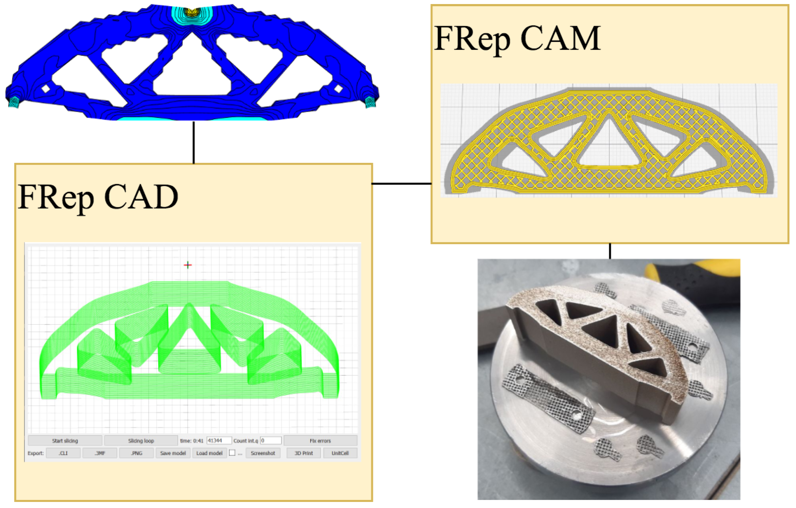
3.2. The Developed FRep CAD/CAM System

The proposed FRep CAD/CAM system [28] is written in C++ using the Qt Creator environment. 3D solids in the system are defined by implementations of C++ template function with two groups of parameters. The first group consists of current coordinates X, Y, Z. The second is an array used for parametrization of the FRep model. The template engine uses not only built-in data types (float, double), but also allows the use of interval [29] and affine arithmetic [30] to optimize computations [18]. Moreover, the developed system is equipped with the HyperFun interpreter [31] to provide modeling capabilities. Some primitives are implemented as built-in functions, for example, a free-form object used for topology optimization. The performance of the system when working with built-in functions is much higher.
The developed system uses the contouring algorithm from [18] both for visualization and direct slicing. This algorithm uses MS approach on regular and adaptive grids. Users can choose interval or affine arithmetic for grid adaptation, and use finer grids at the boundary. The effect of adaptive grids is significant when a task requires high accuracy. According to [18] the system performs contouring up to six times faster on adaptive grids than on regular ones. This can be observed on grids with cells 500 times smaller than model sizes.
The system translates generated contours into G-codes, or exports them into STL files. The support of STL format is necessary as some 3D printing equipment has proprietary G-code protocols. Therefore, two manufacturing scenarios can be implemented—direct slicing and STL-based slicing. The second option is slower. According to [19] on some models the direct slicing runs up to 300 times faster than STL-based one.
The developed system has other advantages of FRep. Models created in the system are fully parameterized and have no cracks, overhangs and inverted faces. Moreover, the size of files with models is significantly smaller. For example, the model shown in Figure 4 occupies near 30 KB as an FRep defining function. The same model in STL format occupies approximately 100 MB, which is 3000 times more. This difference increases dramatically with increasing complexity of topology or in the case of porous models.
This system has a broad set of applications. FRep is more attractive in applications where models have microstructures. These models require high precision when they have a small feature size. Complex models with such qualities appear in natural gas separation. Therefore, our system can be applied in this field [32]. Moreover, similar models exist in the implantation [33]. The use of our software for the design of topologically optimal implants seems attractive.

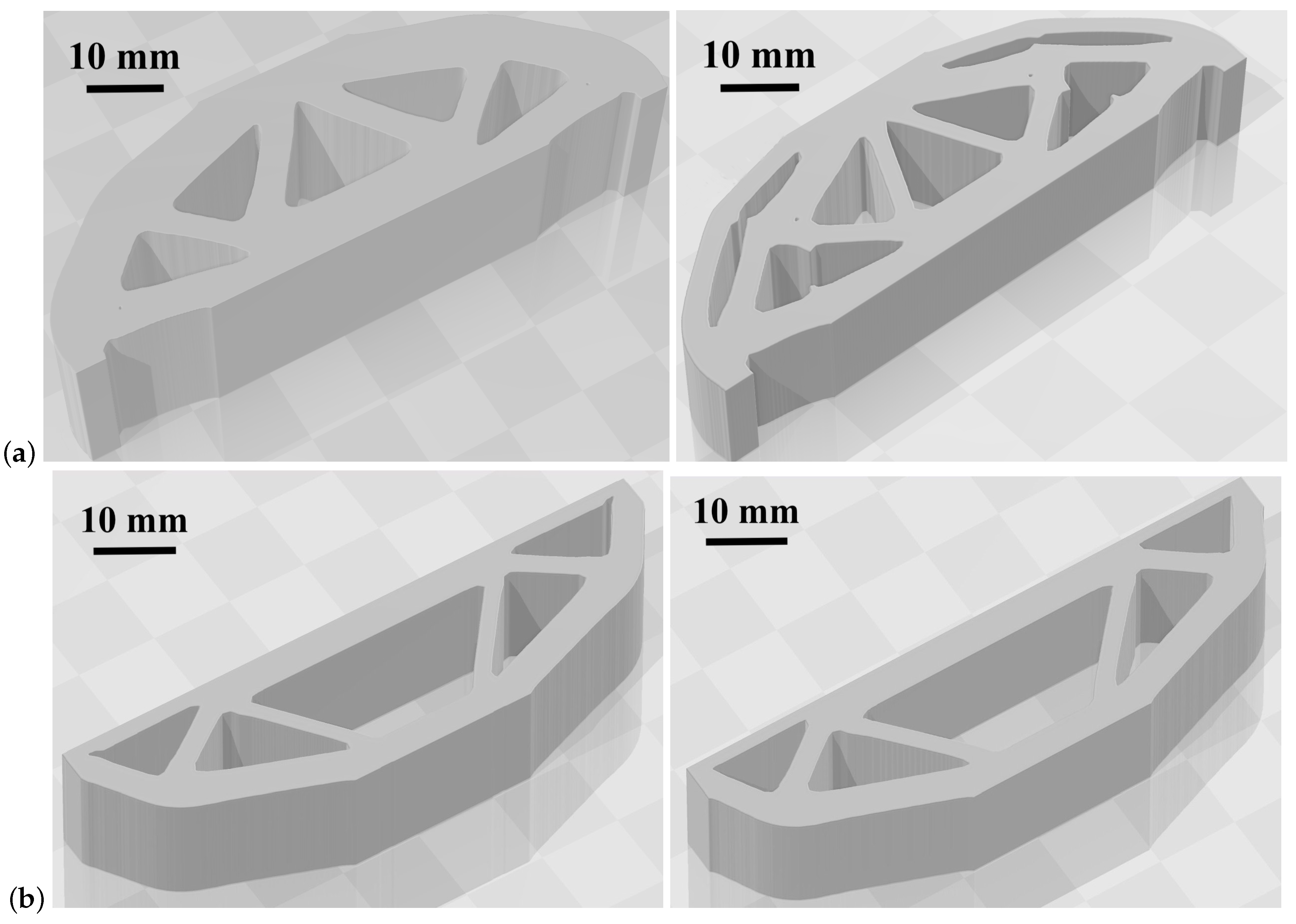
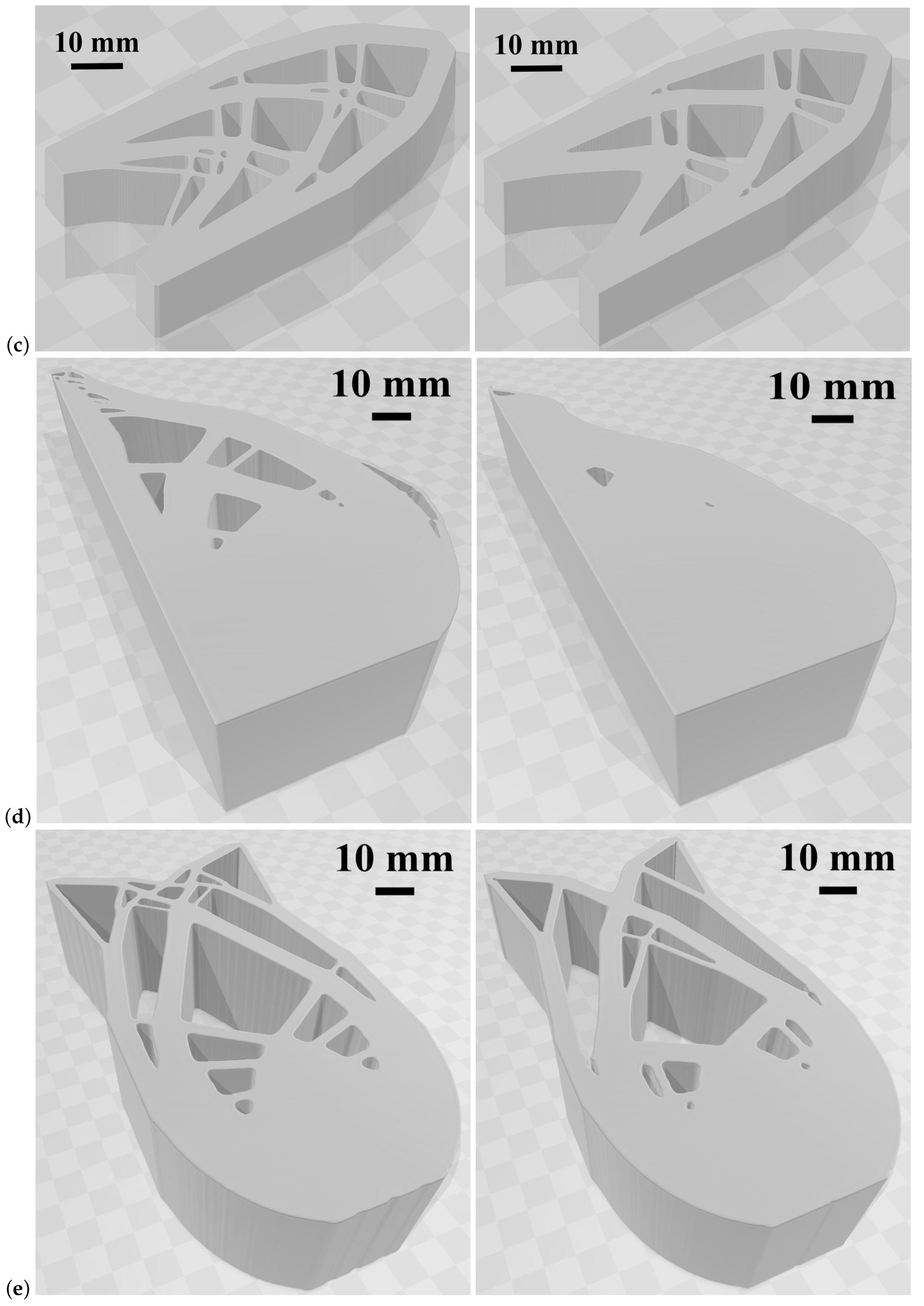
3.3. Results of the Experimental Validation

To validate the developed FRep CAD/CAM system, we printed the part shown in Figure 7a left, and conducted its mechanical testing. Dimensions of the printed part (Figure 9a) are 86 × 25 × 20 mm. The part was cut from the substrate and tested in the three-point bending mode (Figure 9b) at the Instron 5969 testing machine.
Results of the experimental validation are presented as load-displacement curves for several control points. The vertical component of displacement is used in these curves. The obtained load-displacement curve for point P3 (Figure 9c) is presented as red dots in Figure 9f. Computed results for the same load are presented as the solid red line. One can clearly see the disagreement between computational and experimental data.
This discrepancy between the analytical and experimental results of the red lines can be attributed to flutes (Figure 9c) manufactured to increase the stability of the part during the test. A sagging was observed in their areas (Figure 9d) during the testing process. It influenced the load-displacement curve with the displacement value of the whole printed part. The vertical displacement of point P3 was calculated relative to point P0 (Figure 9c) for subtracting the influence of sagging from the load-displacement test curve. Figure 9f shows the load-displacement curves relative to point P0 as green patterns. The correlation between the experimental and predicted results holds up to a load of 15 kN.
During the compression test, it was possible to achieve local plastic deformations. Depending on the distance from P0, the contribution of plastic deformation to the vertical displacement differs. Therefore, additional points, P1 and P2 (Figure 9c), were considered. The computational results for those points are presented in Figure 9e. The correlation between the experimental and computational results for the point P2 is preserved up to the load of 10 kN. For the point P1 the correlation with computational results can be observed up to the load of 5 kN.
We can conclude that the contribution of plastic deformation is the highest in the vicinity of the point P0. The deflection from the elasticity is observed for point P1. It influences the vertical displacements of points P2 and P3. We can conclude that mechanical testing results repeat the theoretical results within the elastic field region, where the computational model was applied. At the loads exceeding 15 kN, the contribution of plasticity starts to grow, and it becomes impossible to compare the computational and experimental results obtained during optimization. At the same time, this experimental validation showed that the proposed approach can be freely used for 3D printed parts that are made up of ceramics [34] and other materials without plastic deformation.
Moreover, we can compare the experimental value of the work done by the applied force and the theoretical values of elastic deformation energy. The upper limit of elastic deformations was observed at the point P3 at the load of 15 kN. This point lies in the vicinity of the loaded point of the body. Therefore, we can calculate an approximate value of the work done by the applied force as follows:
A = F d 2
where F is the load and d is the deformation at a given point. The load equals 15 kN, d equals 0.053 mm. Thus, the work A equals 0.4 J. The FEM routine of Algorithm 1 provides the same value of elastic energy at these load and dimensions of the printed part.

4. Conclusions

This paper proposes the FRep-based CAD/CAM system for additive manufacturing. The FRep geometric kernel provides several opportunities for design, analysis and topology optimization. The efficient and robust topology optimization algorithm was developed for the system. The algorithm is based on the level-set method in combination with the defining function of FRep geometry. The proposed algorithm runs up to 100 times faster than the original algorithm, depending on the boundary conditions and the grid size. The interface to 3D printers, implemented in the system, allows manufacturing of functional parts with desired mechanical properties directly from the CAD/CAM system. The validation performed shows the fitness of the simulation model and its ability to accurately predict the elastic deformations of the manufactured part at control points. Moreover, the validation has also shown the directions for further development of the system.
In future research, authors intend to add the automatic generation of supports to the direct slicing algorithm. The optimization algorithm will be updated to operate with several materials and anisotropic materials. In the next version of the system, the analysis procedure will include the model of plasticity. These revisions will allow us to study how printing conditions influence objective functions of optimized parts. Different regimes of 3D printing affect the anisotropic properties of the material. We plan to study their impact on topology optimization.

Author Contributions

Methodology, D.P., S.E. and A.P.; software, D.P. and E.M.; validation, Y.K.; formal analysis, D.P. and Y.K.; writing—original draft preparation, D.P. and Y.K.; writing—review and editing, E.M., A.P., A.S. and S.E.; visualization, D.P., Y.K. and A.S.; supervision, A.P.; project administration, I.A. All authors have read and agreed to the published version of the manuscript.

Funding

This research received no external funding.

Institutional Review Board Statement

Not applicable.

Informed Consent Statement

Not applicable.

Data Availability Statement

The data presented in this study are openly available in FigShare at https://doi.org/10.6084/m9.figshare.15142209.v1.

Acknowledgments

The authors kindly thank employees of the Center for Design, Materials and Manufacturing of Skoltech Stepan Konev for conducting the mechanical test and consulting with the experimental part of the research and Boris Fedulov for consulting with the simulation and result analysis. This research is funded by the Skoltech Institute of Science and Technology (Skoltech). The authors also would like to thank the anonymous reviewers for their thoughtful and detailed comments on our paper.

Conflicts of Interest

The authors declare no conflict of interest.

Abbreviations

The following abbreviations are used in this manuscript:
AMAdditive manufacturing
BRepBoundary representation
CADComputer-aided design
CAMComputer-aided manufacturing
CNCcomputer numerical control
DLPDigital light processing
DMDDirect metal deposition
FFFFused filament fabrication
FRepFunction representation
MSMarching squares
PDEPartial differential equations
SIMPSolid isotropic material with penalization

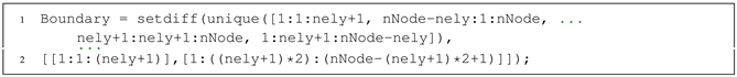
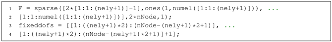
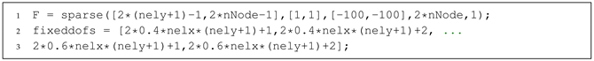
Appendix A. MATLAB Implementation of the Optimization Algorithm

Applsci 11 07409 i001
Applsci 11 07409 i002

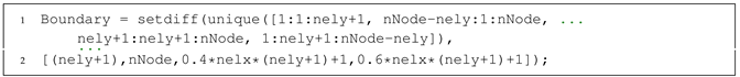
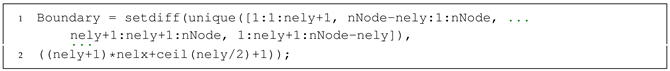
Appendix B. Modifications of the Optimization Algorithm

There are changes to achieve model Figure 7b.
Lines 14–15:
Applsci 11 07409 i003
Lines 31–32:
Applsci 11 07409 i004
There are changes to achieve model Figure 7c.
Line 1:
Applsci 11 07409 i005
Lines 14–15:
Applsci 11 07409 i006
Lines 31–32:
Applsci 11 07409 i007
There are changes to achieve model Figure 7d.
Line 1:
Applsci 11 07409 i008
Lines 14–15:
Applsci 11 07409 i009
Lines 31–32:
Applsci 11 07409 i010
There are changes to achieve model Figure 7e.
Line 1:
Applsci 11 07409 i011
Lines 14–15:
Applsci 11 07409 i012
Lines 31–32:
Applsci 11 07409 i013

References

  1. Zhang, B.; Goel, A.; Ghalsasi, O.; Anand, S. CAD-based design and pre-processing tools for additive manufacturing. J. Manuf. Syst. 2019, 52, 227–241. [Google Scholar] [CrossRef]
  2. Gisario, A.; Kazarian, M.; Martina, F.; Mehrpouya, M. Metal additive manufacturing in the commercial aviation industry: A review. J. Manuf. Syst. 2019, 53, 124–149. [Google Scholar] [CrossRef]
  3. Kumar, V.; Dutta, D. An assessment of data formats for layered manufacturing. Adv. Eng. Softw. 1997, 28, 151–164. [Google Scholar] [CrossRef]
  4. Schumacher, C.; Bickel, B.; Rys, J.; Marschner, S.; Daraio, C.; Gross, M. Microstructures to Control Elasticity in 3D Printing. ACM Trans. Graph. 2015, 34. [Google Scholar] [CrossRef] [Green Version]
  5. Vilbrandt, C.; Pasko, G.; Pasko, A.; Fayolle, P.A.; Vilbrandt, T.; Goodwin, J.R.; Goodwin, J.M.; Kunii, T.L. Cultural Heritage Preservation Using Constructive Shape Modeling. Comput. Graph. Forum 2004, 23, 25–41. [Google Scholar] [CrossRef]
  6. Pasko, A.; Adzhiev, V.; Sourin, A.; Savchenko, V. Function representation in geometric modeling: Concepts, implementation and applications. Vis. Comput. 1995, 11, 429–446. [Google Scholar] [CrossRef]
  7. Rvachev, V. Method of R-functions in boundary-value problems. Sov. Appl. Mech. 1975, 11, 345–354. [Google Scholar] [CrossRef]
  8. Sourin, A.I.; Pasko, A.A. Function representation for sweeping by a moving solid. IEEE Trans. Vis. Comput. Graph. 1996, 2, 11–18. [Google Scholar] [CrossRef]
  9. Pasko, G.; Pasko, A. Trimming implicit surfaces. Vis. Comput. 2004, 20, 437–447. [Google Scholar] [CrossRef]
  10. Pasko, G.; Pasko, A.; Kunii, T. Space–time blending. Comput. Animat. Virtual Worlds 2004, 15, 109–121. [Google Scholar] [CrossRef]
  11. Rvachev, V.L.; Sheiko, T.I.; Shapiro, V. Application of the method of R-functions to integration of differential equations with partial derivatives. Cybern. Syst. Anal. 1999, 35, 1–18. [Google Scholar] [CrossRef]
  12. Chen, J.; Shapiro, V.; Suresh, K.; Tsukanov, I. Shape optimization with topological changes and parametric control. Int. J. Numer. Methods Eng. 2007, 71, 313–346. [Google Scholar] [CrossRef]
  13. Gibou, F.; Fedkiw, R.; Osher, S. A review of level-set methods and some recent applications. J. Comput. Phys. 2018, 353, 82–109. [Google Scholar] [CrossRef]
  14. Van Dijk, N.P.; Maute, K.; Langelaar, M.; Van Keulen, F. Level-set methods for structural topology optimization: A review. Struct. Multidiscip. Optim. 2013, 48, 437–472. [Google Scholar] [CrossRef]
  15. Wang, Y.; Luo, Z.; Kang, Z.; Zhang, N. A multi-material level set-based topology and shape optimization method. Comput. Methods Appl. Mech. Eng. 2015, 283, 1570–1586. [Google Scholar] [CrossRef]
  16. Safonov, A.A. 3D topology optimization of continuous fiber-reinforced structures via natural evolution method. Compos. Struct. 2019, 215, 289–297. [Google Scholar] [CrossRef]
  17. Goh, G.; Toh, W.; Yap, Y.; Ng, T.; Yeong, W. Additively manufactured continuous carbon fiber-reinforced thermoplastic for topology optimized unmanned aerial vehicle structures. Compos. Part B Eng. 2021, 216, 108840. [Google Scholar] [CrossRef]
  18. Popov, D.; Maltsev, E.; Fryazinov, O.; Pasko, A.; Akhatov, I. Efficient contouring of functionally represented objects for additive manufacturing. Comput. Aided Des. 2020, 129, 102917. [Google Scholar] [CrossRef]
  19. Song, Y.; Yang, Z.; Liu, Y.; Deng, J. Function representation based slicer for 3D printing. Comput. Aided Geom. Des. 2018, 62, 276–293. [Google Scholar] [CrossRef]
  20. Wei, P.; Li, Z.; Li, X.; Wang, M.Y. An 88-line MATLAB code for the parameterized level set method based topology optimization using radial basis functions. Struct. Multidiscip. Optim. 2018, 58, 831–849. [Google Scholar] [CrossRef]
  21. Lopes, H.; Oliveira, J.B.; de Figueiredo, L.H. Robust adaptive polygonal approximation of implicit curves. Comput. Graph. 2002, 26, 841–852. [Google Scholar] [CrossRef]
  22. Olszta, P.W.; Umbach, A.; Baker, S.; Fay, J.F.; Tsiombikas, J.; Niehorster, D.C. The Free OpenGL Utility Toolkit. 2019. Available online: http://freeglut.sourceforge.net (accessed on 10 August 2021).
  23. Jamieson, R.; Hacker, H. Direct slicing of CAD models for rapid prototyping. Rapid Prototyp. J. 1995, 1, 4–12. [Google Scholar] [CrossRef]
  24. Ultimaker. CuraEngine. 2013. Available online: https://github.com/Ultimaker/CuraEngine (accessed on 10 August 2021).
  25. Kuzminova, Y.; Firsov, D.; Konev, S.; Dudin, A.; Dagesyan, S.; Akhatov, I.; Evlashin, S. Structure control of 316L stainless steel through an additive manufacturing. Lett. Mater. 2019, 9, 551–555. [Google Scholar] [CrossRef] [Green Version]
  26. Standard Test Methods for Tension Testing of Metallic Materials; ASTM International Standard: West Conshohocken, PA, USA, 2021.
  27. Standard Test Methods for Flexural Properties of Unreinforced and Reinforced Plastics and Electrical Insulating Materials; ASTM International Standard: West Conshohocken, PA, USA, 2017.
  28. Skoltech. FRepCADCAM. 2020. Available online: https://github.com/Torrero/FRepCAM (accessed on 10 August 2021).
  29. Moore, R. Interval Analysis; Prentice-Hall: Englewood Cliff, NJ, USA, 1966. [Google Scholar]
  30. Stolfi, J.; Figueiredo, L. An Introduction to Affine Arithmetic. Trends Appl. Comput. Math. 2003, 4, 297–312. [Google Scholar] [CrossRef]
  31. Digital Materialization Group. HyperFun Project Description. 2014. Available online: http://hyperfun.org/ (accessed on 10 August 2021).
  32. Maltsev, E.; Popov, D.; Chugunov, S.; Pasko, A.; Akhatov, I. An Accelerated Slicing Algorithm for Frep Models. Appl. Sci. 2021, 11, 6767. [Google Scholar] [CrossRef]
  33. Safonov, A.; Maltsev, E.; Chugunov, S.; Tikhonov, A.; Konev, S.; Evlashin, S.; Popov, D.; Pasko, A.; Akhatov, I. Design and Fabrication of Complex-Shaped Ceramic Bone Implants via 3D Printing Based on Laser Stereolithography. Appl. Sci. 2020, 10, 7138. [Google Scholar] [CrossRef]
  34. Safonov, A.; Chugunov, S.; Tikhonov, A.; Gusev, M.; Akhatov, I. Numerical simulation of sintering for 3D-printed ceramics via SOVS model. Ceram. Int. 2019, 45, 19027–19035. [Google Scholar] [CrossRef]
Figure 1. The principal components of the FRep system.
Applsci 11 07409 g001
Figure 2. Bilinear spline construction: (a) the surface defined by the bilinear spline basis function (4); (b) the surface produced by two spline basis functions and its zero-level set (boundary); (c) rectangular domain D with 90 × 25 elements and 91 × 26 knots.
Applsci 11 07409 g002
Figure 3. Union and set difference operations on functionally defined disks.
Applsci 11 07409 g003
Figure 4. Visualization of an FRep model layer by layer.
Applsci 11 07409 g004
Figure 5. The infill patterns: (a) grid, (b) lines.
Applsci 11 07409 g005
Figure 6. Realized components of the FRep system.
Applsci 11 07409 g006
Figure 7. Optimal geometries obtained with modified algorithm (left) and original algorithm (right) (see Section 3.1): (a) the three-point bending beam optimization case; (b) the optimization case where the beam is supported horizontally in two bottom points, and equal loads applied vertically in upper corners; (c) the cantilever beam optimization case; (d) the optimization case where the beam is fixed along the bottom side, and the horizontal load linearly distributed along the left side of the beam; (e) the optimization case where the beam is fixed horizontally in two bottom points, and equal loads applied horizontally in upper corners.
Applsci 11 07409 g007aApplsci 11 07409 g007b
Figure 8. The experimental test design.
Applsci 11 07409 g008
Figure 9. (a) The manufactured part attached to the cylindrical substrate. (b) The image from Digital Image Correlation System. (c) The location of tracked points on the part. (d) The test photos of the part under loads 0 and 15 kN. (f) The test and calculation results of vertical displacement for points P1 and P2. (e) The test and calculation results of vertical displacement for point P3.
Applsci 11 07409 g009aApplsci 11 07409 g009b
Figure 10. Optimization cases and initial assumptions: (a) the three-point bending beam case; (b) the beam is supported horizontally in two bottom points, and equal loads applied vertically in upper corners; (c) the cantilever beam case; (d) the beam is fixed along the bottom side, and the horizontal load linearly distributed along the left side of the beam; (e) the beam is fixed horizontally in two bottom points, and equal loads applied horizontally in upper corners.
Applsci 11 07409 g010
Table 1. Results of algorithms comparison.
Test NumberModified Algorithm, sWei’s Algorithm, s
136.880.8
235.277.3
336.181.7
435.975.8
535.276.6
635.977.3
735.476.2
835.576.4
935.976.1
1036.376.8
Average time, s35.877.5
Number of iterations213179
Objective function1.71 × 10 5 1.71 × 10 5
Volume0.450.45
Table 2. Efficiency of algorithms for four cases.
CaseTimeObjective Function
Modified Algorithm, sWei’s Algorithm, sModified AlgorithmWei’s Algorithm
Figure 10b21.951.91.06 × 10 6 1.06 × 10 6
Figure 10c22.2448.66.00 × 10 5 6.02 × 10 5
Figure 10d165.214902.21.47 × 10 10 1.59 × 10 10
Figure 10e24.4437.12.48 × 10 7 2.48 × 10 7
Publisher’s Note: MDPI stays neutral with regard to jurisdictional claims in published maps and institutional affiliations.

