Numerical Characterization of the Solid Particle Accumulation in a Turbulent Flow through Curved Pipes by Means of Stokes Numbers

Featured Application

This work indicates that the level of particle concentration in curved pipes can be predetermined by Stokes Numbers and; therefore, in the future it should be considered in the study of industrial problems such as thickness losses in high pressure pipes that it transports fluids with solids in suspension, food transport through air and in interchangers with multiphase flows.

Abstract

The accumulation of particles in a turbulent flow of incompressible air with mono-dispersed solid particles inside a 90° pipe bend was simulated using ANSYS^® Fluent (CFD), taking into account the effect of gravity, drag force and a bidirectional fluid-particle coupling. An analysis of the geometrical parameters and the structures of the secondary flow generated in a curved pipe (Dean vortices) was developed, thus determining the characteristic time scales of the flow. Four Stokes numbers (Stk) were formulated, whose values are calculated and studied from the numerical simulations performed. Two different particle sizes (d1 = 50 μm y d2 = 150 μm), at two different flow conditions (Re1 = 61,500 y Re2 = 173,972), and for three curvature ratios Rc/R = 1, 4 and 8 were studied. The flow was solved using a Eulerian–Lagrangian approach with a RNG k-ε turbulence model. Once the multiphase flow was solved and validated, the distribution and maximum particle concentration inside the 90° bend were presented. Additionally, the Stk numbers were calculated to estimate the possible particle concentration level for the different system configurations (dp, Re and Rc/R). It is concluded that, if all Stk numbers are less than one, relative concentration levels reach a minimum, while for Stk numbers larger than one, an increase in the maximum concentration inside the pipe bend was noticed.

1. Introduction

Particle-laden turbulent flows in curved pipes are essential components of almost all industrial process equipment, including power production, chemical and food industries, heat exchangers, nuclear reactors, and engine exhaust ducts, hence understanding their behavior is of great interest. The numerical study of turbulent flow through curved pipes is complex, so there are relatively few reports dealing with the use of numerical methods focusing on the influence of flow conditions and geometry on the accumulation of particles. In 1997, McFarland et al. numerically studied a turbulent flow loaded with solid particles through a 90° bend pipe using RANS (Reynolds Averaged, Navier Stokes Equations) along with the Reynolds stress model to solve the transport phase flow field while accounting for turbulent fluctuations in the equation of motion of the particles. Additionally, they developed an empirical model that considered the influence of Stokes number, Reynolds number and radius on particle accumulation [1]. Breuer et al. (2006) simulated the experimental case treated by Pui et al. (1983) for two Reynolds numbers (Re = 1000 and 10,000) and several particle sizes using Large Eddy Simulation (LES) to solve the transport phase and a Lagrangian tracking model to solve the particle motion, obtaining acceptable results [2,3].

Zhang et al. (2012) carried out a systematic numerical study to generate the computational guidelines to model and validate the turbulent flow through curved pipes by means of RANS equations and Lagrangian tracking, using the commercial code ANSYS FLUENT [4]. Recently, Noorani et al. (2016) investigated the effect of curvature on particle distribution in a multiphase turbulent flow through a curved pipe, for this purpose they used DNS and Lagrangian tracking, for Re = 11,700 and three different radii of curvature [5]. Finally, Guda et al. (2017) conducted a study on the formation of strings (deposition lines) of solid particles in gas flows through sharp turns (bends). Experiments were conducted in which high-speed videos were recorded and analyzed for solid concentration profiles that were compared with CFD simulations using LES and RANS turbulence models; in both simulations and experiments, flows with solid loadings of 35%, 42% and 51% were considered. The results of the study demonstrate that both RANS and LES can accurately predict particle string formation. Additionally, a strong relationship between local solids concentration and gas vorticity was observed [6].

Overall, different numerical studies have been carried out to explore the effect of geometry and flow characteristics on the accumulation of particles in curved pipes. However, there was no evaluation based on the Stokes number, as no formulation of it adapted to the geometry and the physical characteristics of turbulent flow in bends is available. For this reason, in this study a methodology for predicting the degree of accumulation in concentration of solid particles in a 90° bend pipe by means of Stokes numbers specifically formulated for that configuration.

The document is organized as follows. First, in Section 2, we describe the physical model, the validation of the numerical method, and the ad hoc formulated Stokes numbers. In Section 3, we show the distribution and concentration of particles generated in the bend pipe (for the reference case C12d1) and discuss the effect of the indicated parameters (dp, Re, Rc/R) at the point of maximum concentration and possible accumulation mechanism. This is followed by the numerical characterization by means of the Stokes numbers, and the general accumulation conditions are identified. The last section summarizes the main results and conclusions.

2. Physical Modelling and Numerical Methodology

2.1. Numerical Simulation

The computational domain consisted of an inlet pipe of constant diameter and length L₁ followed by a 90° bend (elbow), and an outlet pipe of constant radius and length L₂ (see Figure 1). L₁ is obtained from Equation (1), which defines the development length according to the flow regime. L₂ is defined as 50 pipe diameters to ensure that the effects of the secondary flow disappear before the outlet [7]. The bending ratio is defined as Rc/D in the numerical validation and Rc/R in the study cases, where Rc is the radius of curvature and R is the radius of the pipe.

$$\mathrm{L}=4.4{ \mathrm{Re}}^{\frac{1}{6}}\mathrm{D}$$

(1)

Z′ − Z, θ and R: Represent the axial, azimuthal and radial coordinates, respectively, φ: Angle of deflection of the bend (see Figure 1). The particle-laden flow at the inlet is vertical and aligned with the acceleration of gravity, g = −g_z’$\widehat{k}$.

The turbulent flow loaded with solid particles through the pipe bent at 90° was solved by CFD modeling and with the obtained values the ad hoc formulated Stokes numbers were calculated.

It was studied: Two different particle sizes (d1 = 50 μm and d2 = 150 μm), for two dis-tinct flow conditions (Re1 = 61,508 y Re2 = 173,972), and three curvature ratios (Rc/R = 1, 4 and 8). The chosen particle sizes were determined for a dilute flow and according to the response time of the particle in a tracer flow for a Stk < 1 (not to be confused with the Stk formulated specifically for the flow in an elbow, but rather as classic definition of the number of stokes defined by average flow velocity and pipe diameter). In this work, nine different geometric configurations were simulated: Three cases correspond to this validation section (

Table 1. Dimensions pipeline validation cases.

Case	$\mathbf{D}$	${\mathit{L}}_1 \left[\mathbf{mm}\right]$	${\mathit{L}}_2 \left[\mathbf{mm}\right]$	${\mathbf{R}}_{\mathbf{c}} \left[\mathbf{mm}\right]$	θ [°]
Zhang	104	30D	50D	2D	90
Guda *	76.2	5D	30D	1.8D	90

* Guda case maintains original geometry and is solved for a mass load of 0.35 and 0.42.

), and the other six were used to evaluate the relationship between Stokes numbers and particle accumulation (see Section 2.4).

Flow Properties. The properties of the gas (air) and particles (seeds) are presented in

Table 2. Fluid phase and dispersed phase properties.

Material	$\mathit{\mu }$ [Pa·s]	$\mathit{\rho }$ [kg/m3]	$\mathit{T}$ [K]	Shape	Shape Factor [-]	Sizes [µm]
Air	1.802 × 10−5	1.225	288.73	-	-	-
Particles	-	2710	-	Non-spherical	0.755	d1 = 50	d2 = 150

.

Boundary Conditions. Boundary conditions of velocity at the inlet, pressure (atmospheric) at the outlet and no-slip condition at the wall were imposed. The initial velocity is determined from a plane profile with hybrid initialization, solving the Laplace equation. A fully elastic shock condition and a coefficient of restitution for the particles was set at 1. We considered non-reactive, isothermal, and incompressible flow (low Mach number).

2.1.1. Equations for Fluid Phase and Flow Solver

The fluid phase is described using a Eulerian approach in which the RANS equations are solved. When considering a transient flow in the present study, strictly speaking, URANS equations are solved. Equation (2) is the continuity equation and Equation (3) is the Reynolds averaged quantity of motion equation. Here, F_i is the external body force that arises due to interaction with the dispersed phase, and $g_i$ is the gravitational acceleration vector.

$$\frac{\partial U_i}{\partial x_i}=0$$

(2)

$$\frac{\partial U_i}{\partial t}+U_{j }\frac{\partial U_i}{\partial x_j}=-\frac{1}{\rho }\frac{\partial P}{\partial x_i}+\frac{\partial }{\partial x_j}\left(\nu \frac{\partial U_i}{\partial x_j}\right)-\frac{\partial }{\partial x_j}\langle u_i^{\prime }{u}_j^{\prime }\rangle +{\mathit{g}}_{\mathit{i}}+{\mathit{F}}_{\mathit{i}}$$

(3)

The model describing the transport of mean properties of turbulent flows for the scales being modeled will be the RNG k-ε model. The model offer balance and good “hit rates” when compared to others, as shown by Kim et al. [8]. The RNG k-ε model has governing equations like the standard k-ε model, expressed in a turbulence energy transport equation “k” (Equation (4)) and a dissipation rate “ε” (Equation (5)).

$$\frac{\partial \left(\rho k\right)}{\partial t}+\frac{\partial \left(\rho U_{i}k\right)}{\partial x_i}=\frac{\partial }{\partial x_j}\left[{\alpha }_k{\mu }_{eff}\frac{\partial k}{\partial x_j} \right]-\rho \epsilon +G_k+G_b-Y_M+S_k$$

(4)

$$\frac{\partial \left(\rho \epsilon \right)}{\partial t}+\frac{\partial \left(\rho U_i\epsilon \right)}{\partial x_i}=\frac{\partial }{\partial x_j}\left[{\alpha }_{\mathsf{\epsilon }} {\mu }_{eff}\frac{\partial \epsilon }{\partial x_j} \right]+C_{1\epsilon }\frac{\epsilon }{k}\left( G_k+C_{1\epsilon }{G}_b\right)-C_{2\epsilon }\rho \frac{{\epsilon }^2}{k}-R_{\mathsf{\epsilon }}+S_{\mathsf{\epsilon }}$$

(5)

The RNG k-ε model is obtained using a statistical technique called renormalization group theory that is derived from the instantaneous Navier-Stokes equations, from which analytical derivative results are derived in a model with constants $C_{\mu }$ = 0.0845, $C_{1\epsilon }$ = 1.42, $C_{2\epsilon }$ = 1.68.

2.1.2. Equations for the Dispersed Phase and Lagrangian Particle Tracking

The discrete phase is solved by Lagrange tracking, where the motion of the particles is described by a set of ordinary differential equations for particle position ${\mathit{x}}_{\mathit{p}}$ and velocity ${\mathit{u}}_{\mathit{p}}$. Considering the drag force and particle inertia [9], these equations in vector form read as:

$$\frac{d{\mathit{x}}_{\mathit{p}}}{dt}={\mathit{u}}_{\mathit{p}}$$

(6)

$$\frac{d{\mathit{u}}_{\mathit{p}}}{dt}=\mathit{g}-\frac{\left(1+0.15R{e}_p^{0.687}\right)}{{\tau }_p}\left({\mathit{u}}_{\mathit{p}}-\mathit{u}\right)$$

(7)

where $\mathit{u}$ is the fluid velocity at the particle position, $\mathit{g}$ is the gravitational acceleration vector and ${\tau }_p={\rho }_p{d}_p^2/18\mu$ is the particle relaxation time ($d_p$ and $\mu$ being the diameter of the particle and the dynamic viscosity of the fluid, respectively). The Stokes drag coefficient is computed by using a standard non-linear correction required when the particle Reynolds number, $\mathrm{R}{\mathrm{e}}_p=\left|\mathit{u}-{\mathit{u}}_{\mathit{p}}\right|d_p/\nu$ does not remain small.

2.1.3. Numerical Methods and Setup

The numerical simulations in this study were performed using the commercial package ANSYS^® Fluent (CFD), considering an Eulerian–Lagrangian approach with two-way coupling as the solution method. The Finite Volume Method (FVM) was used for the domain, where the fluid phase is solved for transient and isothermal flow, using the segregated pressure-based algorithm and semi-implicit method for pressure-linked equations (SIMPLE). The transport equations for k and ε are discretized using a Second Order Upwind scheme. This is combined with a correction equation for the pressure derived from the continuity equation and the momentum equation, that is discretized using the PRESTO! scheme (Pressure Staggering Option), which is suitable for flows with strong streamline curvatures. A hybrid initialization was implemented, solving the Laplace equation from the boundary conditions to determine the initial velocity and pressure field. In the simulations, an adaptive time step was used for the fluid phase with a Courant number of 0.5. For the discrete phase, the Courant number is set to 1, and the equation is solved using a Runge–Kutta scheme with the linearized source terms.

For a proper convergent solution, the admissible local error in the residual (cell level) was set to ${10}^{-11}$, and the convergence criterion of the global residual was ${10}^{-5}$ for the continuity equation, and ${10}^{-6}$ for the other equations. The time interval of the simulation is subject to the following criteria: (i) the difference of the mass flow rate between the pipe inlet and outlet should be below ${10}^{-5}$, (ii) stabilisation of the pressure drop along the pipe, (iii) convergence of the average velocity at the pipe outlet, (iv) convergence of $y^{+}$, and (v) the mass flow rate of uniformly injected particles at the inlet of the pipe is like that at the outlet.

Explanation and details of the simulation: Once the transport phase flow has been initialized, the ANSYS Fluent temporal integration scheme proceeds with an adaptive time step for a Courant number of 0.5 as mentioned: With the residuals falling, the time step is set at 0.001 until the residuals stabilize in the order of ${10}^{-5}$ for the continuity equation and, ${10}^{-6}$ for the impulse equation as for the dissipation and kinetic energy equations (the $y^{+}$ is monitored preventively within the range of the logarithmic layer). Then, a solution period “t_e” required to achieve a stable statistical flow is defined, for this the pressure drop in the elbow and the velocity profile in the cross section at the outlet of the pipe are monitored. Once the flow field of the transport phase is resolved, the Lagrangian module or “DPM” of FLUENT is attached and continuous injection of particles is started. Said injection continues for a travel time “t_r” until the mass flow of particles that enters the domain in each time interval is like that of the output, then, when a “stationary” condition is reached in the flow of particles, the statistics—Data Sampling for Time Statistics—are collected, for a sampling time “t_m” equivalent to two runs of the pipe. It is worth mentioning that the total number of particles inside the pipe when a constant flow is achieved is approximately 550,000 particles (depending on the case). The times used are referential, it should be checked if the five criteria mentioned were achieved.

Table 3. Simulation times. $t_e$ = time for a statistically steady flow,$t_r$ = travel time for a steady flow of particles y $t_m$ = sampling time.

Properties	C11	C12	C13	C21	C22	C23
te [s]	1	1	1	0.75	0.75	0.75
tr [s]	1.5	1.5	1.5	1	1	1
tm [s]	2	2	2	2	2	2

contains the times corresponding to the periods described, specific to the case.

The stability of the numerical calculations, if problematic, was improved by reducing the under-relaxation factor to 0.2 for pressure and 0.5 for momentum [4]. The simulations were parallelized on an Intel^® Core™ i7-7700 CPU @ 3.60Ghz (8 CPUs), with 8 Gb RAM and NVIDIA GeForce GTX video card 970.

2.2. Numerical Validation Study

Since the calculation of the ad hoc Stokes numbers (see Section 2.3) is based on parameters obtained by simulation, the numerical models were thoroughly validated with previously published experimental data [4,6,8,10]. It must be taken into account that the Stokes numbers were formulated under characteristic macroscales, so the important thing is to solve well the large turbulent structures, that is, the Dean vortices and the smaller but considerable scale vortices that form near the nucleus of the pipe because of the local imbalance between the centrifugal force and the pressure gradient [11]. The fluid phase was first validated by replicating the pressure drop in the work of Zhang et al. for gas flow through a curved pipe with Rc = 2D—Re = 61,500 [4] and then with the velocity profiles exposed by Kim [8] and Sudo [10]. However, as mentioned, the RNG k-ε model was used as turbulence closure, due to the better performance shown in the studies by Kim et al. compared to other linear and nonlinear parasitic viscosity turbulence models for curved pipe flows [8], and although there is an inherent problem with models of this type because they do not capture the anisotropic nature of turbulence in this type of flow, this can be circumvented by the benefits of the RNG k-ε model that allows precise closure of large structures for the specific problem, where the RNG k-ε model adds an additional term in its equation ε that improves the accuracy of rapidly deformed flows, as well as including improvements in the precision of parasitic flows and provides an analytical formula for turbulent Prandtl numbers. Finally, as turbulence is generally affected by rotation or eddy in the medium flow, the RNG model in ANSYS Fluent provides an option (Eddy Modification) to account for the effects of eddy or rotation by modifying the turbulent viscosity of properly.

The discrete phase was validated by comparing the experimental concentration results obtained by Guda et al. in gas-solid flows with Rc = 1.8D and Re = 75,327 for mass loads of 0.35 and 0.42. The particle size distribution was carried out as detailed in reference [6]. In the same way that was commented for the fluid phase, there is the problem that by not considering the turbulent fluctuations of the scales not captured by the model, the process of turbulent Lagrangian particle diffusion is significantly affected. However, as explained in the work of [12], that although for a long-term diffusion, we cannot avoid the possibility that the particle escapes from its originally “surrounding” fluid, resulting in a slightly eddy diffusion coefficient reduced particle relative to fluid. This effect is reduced for an increase in ${\mathsf{\rho }}_p/{\mathsf{\rho }}_f$, becoming insignificant for a density ratio of 1000. Furthermore, it should be noted that from the delivery results by Guda et al., it is seen that, although there are variations between the SLE and the RANS results, both can predict the general trends of the string formation observed during the experiments. Thus confirming that the simulations account for the physics of the flow as observed in the experiments.

2.2.1. Validation of the Fluid Phase

We compared the pressure distribution (through the pressure coefficient), axial velocity profiles (upstream of the bend) and velocity iso-contours in cross sections through the bend, with the results reported [4,8,10].

• Pressure Coefficient (Cp)

The pressure coefficient values are shown in Figure 2. The maximum error found by the RNG k-ε model is 9.7% (on the inner side of the curve), much lower than the 26% of the RSM and standard k-ε models, and there is a relative <1% in the maxima of the Cp located at 30° on the inner side and 60° on the outer side of the bend. The results obtained for the pressure field were also satisfactory, with the RNG k-ε model performing better than the models RSM and k-ε reported by Zhang et al. [4].

• Velocity Profile

Figure 3 shows the axial velocity profiles. Uz, r, and z are the axial flow velocity, the pipe radius, and the distance along the axial direction, respectively. For comparison, the coordinates were normalized with respect to the pipe diameter (D) and the average velocity (Ub). The numerical values are consistent with experimental results [8,10]. A small underestimation of the profile is present on the adjacent side of the inner face of the upstream curve between z/D = 0 and z/D = 2 (see lower part of the graph).

• Secondary Flow

A comparison of the flow patterns obtained from the numerical simulations and experiments reported by Sudo et al. (Re = 60,000—Rc = 2D) are presented in Figure 4. Velocity contours normalized by the average flow velocity ($\overline{\mathrm{W}}/\mathrm{Wa}$) are shown as isolines that allow visualizing the pattern and behavior of the secondary flow (Dean vortices), at different angles of the curve, as well as at z/D distance upstream and downstream of the elbow. Because the flow is symmetrical to the midplane, only the lower contour of the velocity contour cross section is shown.

In the simulation gravity acts against the flow in the inlet section, unlike the test performed by Sudo et al. where gravity always acts perpendicular to the flow [10]. Nevertheless, this change of orientation does not have a significant effect on the flow structure (Figure 4b). Regardless the orientation, a strong recirculation of the primary flow in the inner curve is noticeable, as the fluid passes through the closed curve. Secondary flow patterns can be seen in several cross sections of the curve (at φ = 60°, 90°). Sudo et al. report a pair of counter-rotating vortices already defined at 45° deflection (not shown in the image), but in our simulation using the RNG k-ε model it is clearly visible beginning at φ = 50° deflection (also not shown in the image). However, in both cases the vortices are clearly formed at φ = 90° (z/D = 0) [10]. Typically, recirculation leads to a significant pressure drop in the bend, so it is especially important to adequately capture the secondary flow inside a bent pipe. Dean vortices are observed to be fully developed downstream at z/D = 2 and persist until z/D = 10, then propagating to the entire cross section.

According to the results shown, as far as validation is concerned, it is concluded that the proposed computational model complies with the physics of the problem when solving the transport phase; It correctly solves the pressure drop of an elbow, captures very well and greatly the characteristic velocity profiles, both within and downstream of the elbow. Finally, and of great importance, it does manage to reproduce the turbulent pattern of the secondary flow (counter-rotating vortices), which, as stated in the results of this work, are fundamental in the mechanism of accumulation of particles in a curved.

2.2.2. Discrete Phase Validation

Figure 5 shows the concentration profiles at different locations in the horizontal pipe downstream of the 90° bend. The particle concentration was normalized by the maximum concentration at the cross section at z/D = 0, following the methodology proposed in Guda et al. (Re = 75,327—Rc = 1.8D) with a Rosin-Rammler (RR) particle distribution. The distribution of solid particles with a mass loading of 0.35 and 0.42 are considered (Figure 5a,b, respectively) [6].

In Figure 5, the deviations between the experimental profiles [6] and the numerical model can be observed, but the concentration levels and the tendency to the formation of the upstream chord can be captured in a good way by the RNG k-e model. The biggest discrepancy that can be observed is mainly that the maximum of the distribution moves faster towards the center of the pipe than those achieved experimentally by Guda et al. [6], this is directly related to the coefficient of restitution of the particles. However, the general trend and particle accumulation lines observed in the experiments can also be identified in the simulation and by using restitution coefficients ≠ 1, it is perceived that this parameter largely dictates the evolution of the rope of particles upstream of the elbow and not their concentration within the elbow, so it is not relevant in the characterization predicted by the Stokes numbers.

2.2.3. Mesh Sensitivity

The sensitivity of the results was examined using three different meshes: A coarse (345,000 items), a medium (612,500) and a fine (1,510,000). All meshes consisted of hexahedral elements and mesh refinement on the inner wall using standard wall functions (SWF) for Mesh 1 (coarse) and Mesh 2 (medium) and using enhanced wall treatment (EWT) for Mesh 3 (fine). Figure 6 shows the medium and fine mesh, for the axial velocity profile within the curve. The results for the coarse mesh were omitted, as they were poor. The velocity field is well resolved near the inside wall. This is of special interest, as it determines the migratory movement of the particles transported by the flow and their accumulation inside the bend. In short, no critical difference is perceived between the fine and medium mesh, so it can be concluded that the underestimation of the flow in the inside wall mentioned above is due to the model used and that it occurs rather at the exit of the curve (90°), due to the detachment of the flow at the point of curvature of the bend on the internal face, extending its effects upstream.

2.3. Relationship between Stokes Numbers and Particle Accumulation at a 90° Elbow

The Stokes number describes the response of a particle to a specific flow condition by determining how inertial the particle behaves (i.e., whether it behaves as a flow tracer (Stk < 1) or not (Stk > 1)). In its classical form, the Stokes number is defined as the relaxation time of the particle “$t_p$” over the characteristic time of the flow “$t_f$” (Equation (8)).

$$Stk=\frac{t_p}{t_f}$$

(8)

However, for the analysis of particle accumulation, the Stokes number can be inverted, as the Stokes number is used to indicate an accumulation of particles (Stk > 1). The accumulation) occurs according to the inertial capacity of each particle to migrate between streamlines (as non-tracer particles) and finally be deposited in a certain area. The latter depends on the accumulation mechanism, which will be defined by the physics of the problem.

The relevant physical and geometrical effects in a bend pipe were previously investigated [11], and possible characteristic lengths, velocities and/or times of the flow were identified according to the physical problem, leading to four different formulations of the Stokes number based on different time scales of fluid:

• Curved Stokes Number ($St{k}_{curved}$), this number quantifies the effect given by the geometry, where the ratio of radii (Rc/R) and velocities (V_mean/V_max) are inversely proportional [7]. Given this relationship, the effect of geometry can be quantified by the radius of curvature and the maximum velocity generated within the bend $t_1={\mathrm{R}}_{\mathrm{c}}/V_{max}$.

  $$St{k}_{curved}=\frac{t_p}{t_1}=\frac{{\rho }_p{d}_p^2 V_{max}}{18{\mu }_g {\mathrm{R}}_{\mathrm{c}} }$$

  (9)
• Stokes Number of particle transit through the vorticial zone ($St{k}_{ t_r}$), as the accumulation is directly related to the residence time of a particle in the bend, we will have a characteristic time $t_2=L_s/V_{mean}$ representing the average time it would take for a fluid particle to travel a distance equal to the arc length of the bend “L_s”. The shorter the average flow time the longer the particle residence time, favoring particle accumulation.

  $$St{k}_{ t_r}=\frac{t_2}{t_p}=\frac{18{\mu }_g L_s }{{\rho }_p{d}_p^2 V_{mean} }$$

  (10)
• Primary Centrifugal Stokes Number ($St{k}_{ {\omega }_c}$), quantifies the effect of the change of direction, where the particles are affected in their equilibrium position by the centrifugal force caused by the curvature. Then, it will be represented by the response of the particles to the angular velocity (${\omega }_c=V_{mean}/Rc$) measured with respect to the center of curvature that the particle is affected $\left(t_3=1/ {\omega }_c\right)$.

  $$St{k}_{ {\omega }_c}=\frac{t_3}{t_p}=\frac{18{\mu }_g }{{\rho }_p{d}_p^2 {\mathrm{\omega }}_{\mathrm{c}}}=\frac{18{\mu }_g {\mathrm{R}}_{\mathrm{C}}}{{\rho }_p{d}_p^2 V_{mean} }$$

  (11)
  The greater the centrifugal force, the greater the ${\omega }_c$, causing the increase of centrifuged particles to the external face of the elbow, generating greater accumulation in this zone.
• Secondary Centrifugal Stokes Number ($St{k}_{ {\omega }_v}$), aims to quantify the susceptibility of the particle to be centrifuged out of the Dean vortices (secondary flow) towards the central plane and zones of lower vorticity. Therefore, it will be determined by the relative angular velocity that the particles are subjected to with respect to the rotating center of the vortex (${\omega }_v).$ ${\omega }_v$, for simplicity, is calculated from the maximum tangential velocity present in the zone of greatest accumulation within the bend and the radius of the vortex, which is approximately equal to the radius of the pipe $\left({\omega }_v=V_{tang.max}/R\right)$. Because two counter-rotating vortices are present, the expression is multiplied by a factor of 2.

  $$St{k}_{ {\omega }_v}=\frac{2t_4}{t_p}=\frac{36{\mu }_g }{{\rho }_p{d}_p^2 {\omega }_v}=\frac{36{\mu }_g \mathrm{R}}{{\rho }_p{d}_p^2 V_{tang.max}}$$

  (12)

2.4. Study Cases

In this paper, the four ad hoc formulated Stokes numbers were calculated using numerical methods, and their relationship with the maximum concentration formed in a 90° bend, for different configurations was analyzed. A turbulent air flow with a dilute solid phase of mono-dispersed particles (mass load 42%, ${\alpha }_p$ < 10⁻³) was modeled. Two flow conditions Re1 = 61,508 (V₁ = 8.7 [m/s]) and Re2 = 173,972 (V₂ = 24.6 [m/s]), two particle sizes $d_{p1}=50 \left[\mathsf{\mu }\mathrm{m}\right]$ and $d_{p2}=150 \left[\mathsf{\mu }\mathrm{m}\right]$ and three different radii of curvature Rc/R = 1, Rc/R = 4 and Rc/R = 8 were considered, totaling twelve study cases identified according to the code shown in Figure 7. Until now, the Dean number, a dimensionless number that determines flow structures at elbows, had not been introduced. It is defined: De $=\mathrm{Re}\sqrt{\mathrm{D}/2\mathrm{Rc}}$. The Dean number mainly marks the transition from laminar to turbulent flow, determining the internal structure that the secondary flow will manifest, although there is no universal solution since the parameter depends largely on the curvature ratio. According to the literature, a completely turbulent flow can be considered for De > 400 in circular pipes, that is, without vortices that present undulations, twists and eventually fusion and division of pairs. The cases developed, as can be seen in Figure 7, are high, so it can be considered a completely turbulent flow. Although it is important to take into account the Dean number in order to know with which flow one is working, in the present work it was not used as a direct parameter to measure the dependence of the Stokes numbers with the concentration because, as it depends so much on the Reynolds number as in the curvature relationship. For equal Dean numbers (De) it does not show a clear correlation because the weighting of the Reynolds effect and the radius of curvature is not the same for the concentration of particles.

The presented Eulerian–Lagrangian approach was used, where the RNG k-ε model was selected as the method for solving the fluid phase and the ANSYS Fluent discrete phase module for Lagrangian tracking of the particles. Only the effect of the drag force of the flow (air) and the action of gravity were considered on the particles. The interaction between phases was modeled using a bidirectional coupling and fully elastic collisions were considered. According to the diagram of Sommerfield et al. [13], the volume fraction is delimited between ${10}^{-6}<{\alpha }_p<{10}^{-3}$.

The geometrical models are shown in Figure 8.

Table 4. Geometric dimensions in the study cases.

Geometry	$\mathbf{D}$	${\mathit{L}}_1 \left[\mathbf{mm}\right]$	${\mathit{L}}_2 \left[\mathbf{mm}\right]$	${\mathbf{R}}_{\mathbf{c}}/\mathbf{R} [-]$	θ [°]
C11	104	28D	50D	1	90
C12	104	28D	50D	4	90
C13	104	28D	50D	8	90
C21	104	33D	50D	1	90
C22	104	33D	50D	4	90
C23	104	33D	50D	8	90

summarizes the construction parameters.

The domain was discretized using a structured mesh of hexahedral elements whose nodes were equally spaced in azimuthal and axial directions. In the radial direction and in general, the resolution and quality values of the Mesh 2 used in the validation of the transport phase and discrete phase were used (Section 2.2.1 and Section 2.2.2).

Table 5. $\Delta x$ = azimuthal, $\Delta y$ = radial and $\Delta z$ = axial mesh grid size used and the number of elements in each direction N_x, N_y, N_z, respectively. In the radial direction, a mesh refinement was made close to the wall, starting with $\Delta y_{min}$ increasing towards the center until reaching $\Delta y_{max}$ with a growth factor of 1.2.

z	C11	C12	C13	C21	C22	C23
$N_x$ × $N_y$ × $N_z$	56 × 700 × 1000	56 × 700 × 854	56 × 700 × 856	56 × 700 × 1000	56 × 812 × 906	56 × 812 × 938
N° of elements	700,533	597,800	620,200	700,533	735,672	761,656
$\Delta x$ [mm]	5.8	5.8	5.8	5.8	5.8	5.8
$\Delta z$ [mm]	10	10	10	10	10	10
$\Delta y_{min}$ [mm]	1.35	1.35	1.35	1.35	0.54	0.54
$\Delta y_{max}$ [mm]	4.13	4.13	4.13	4.13	3.37	3.37
y+	40	40	40	100	40	40
Aspect Ratio	<12	<7.5	<7.5	<12	<19	<19
Orthogonality	<0.84	<0.63	<0.63	>0.84	>0.66	>0.66
Skewness	<0.45	<0.62	<0.62	<0.45	<0.61	<0.61

shows the number of elements used in each case and their characteristic dimensions, and Figure 9 shows an example of the type of mesh constructed.

3. Results and Discussion

The concentration (Equation (13)) determines the average mass of particles residing per cell, from which it can be concluded that, given an abrupt increase in concentration in a cell, which also remains constant over time, it will represent a zone of particle accumulation.

$$m_{DPM}=\frac{\overline{m_{p,cell}}{ t}_p s_p}{v_{cell}}\left[\mathrm{kg}/{\mathrm{m}}^3\right]$$

(13)

where $\overline{m_{p,cell}}$ is the average particle mass in a cell, $t_p$ is the particle residence time per cell, $v_{cell}$ is the volume of each cell and $s_p$ is the total particle flow rate per cell.

Accumulation statistics studied by concentration and distribution of particles continuously injected from the pipe inlet, were collected between z′ = −1D and z = 3D after a physical travel time t_r = 1.5 [s] and 1 [s] (for a flow velocity V₁ = 8.7 [m/s] and V₂ = 24.6 [m/s], respectively), where a constant flow of particles was achieved. Since the results were extensive due to the number of cases simulated and the variety of parameters studied (dp, Re and R/Rc), they are presented and discussed based on the concentration results of case C12d1. However, the analysis and conclusions made here are formulated always considering all the cases. Complementary information about the other cases is presented in Appendix A.

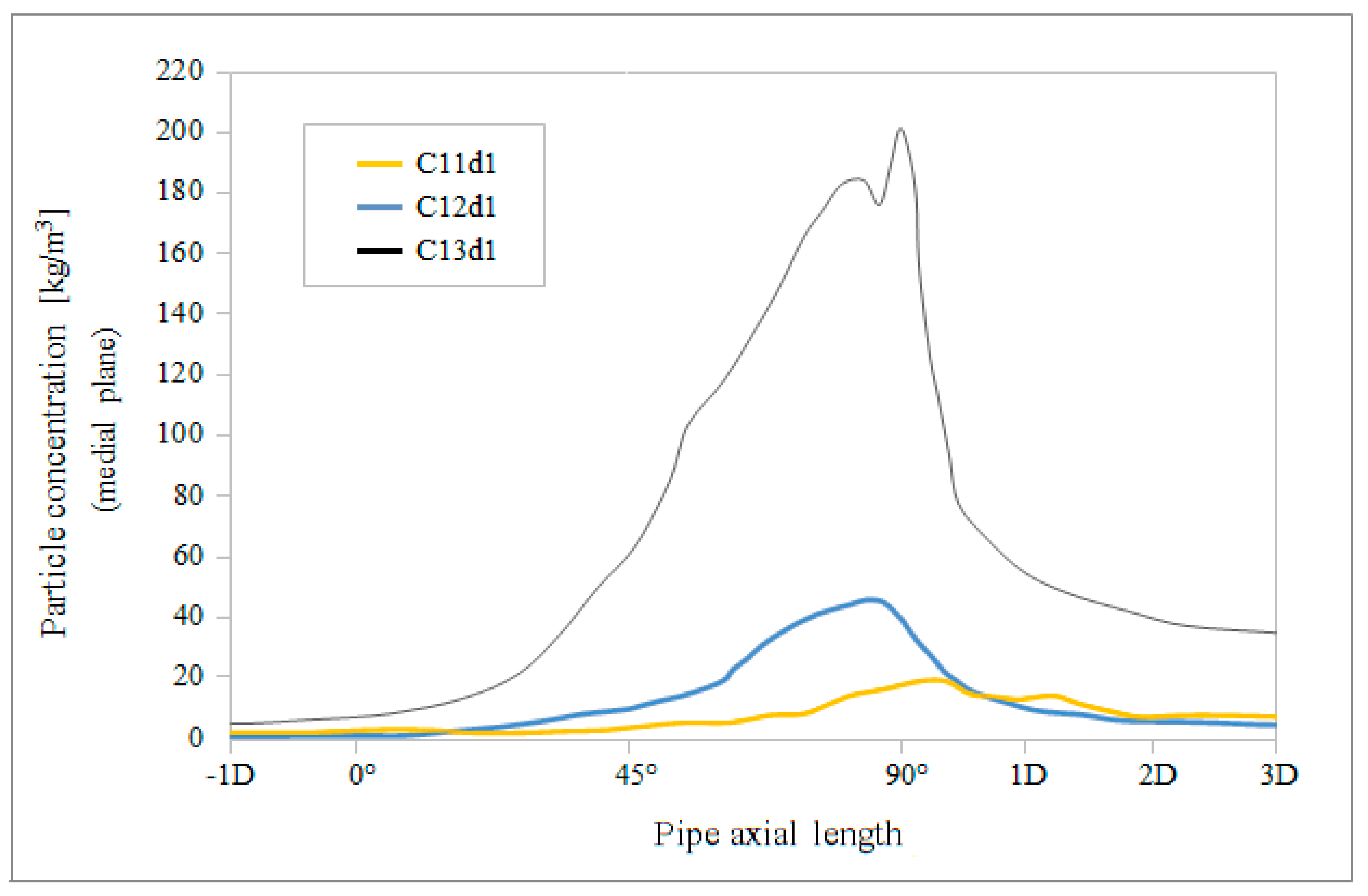
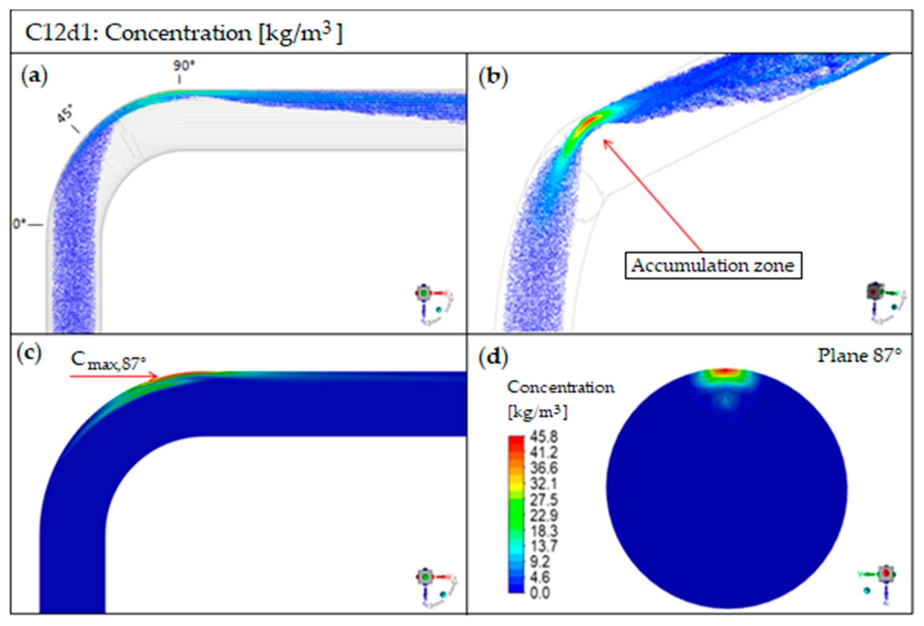
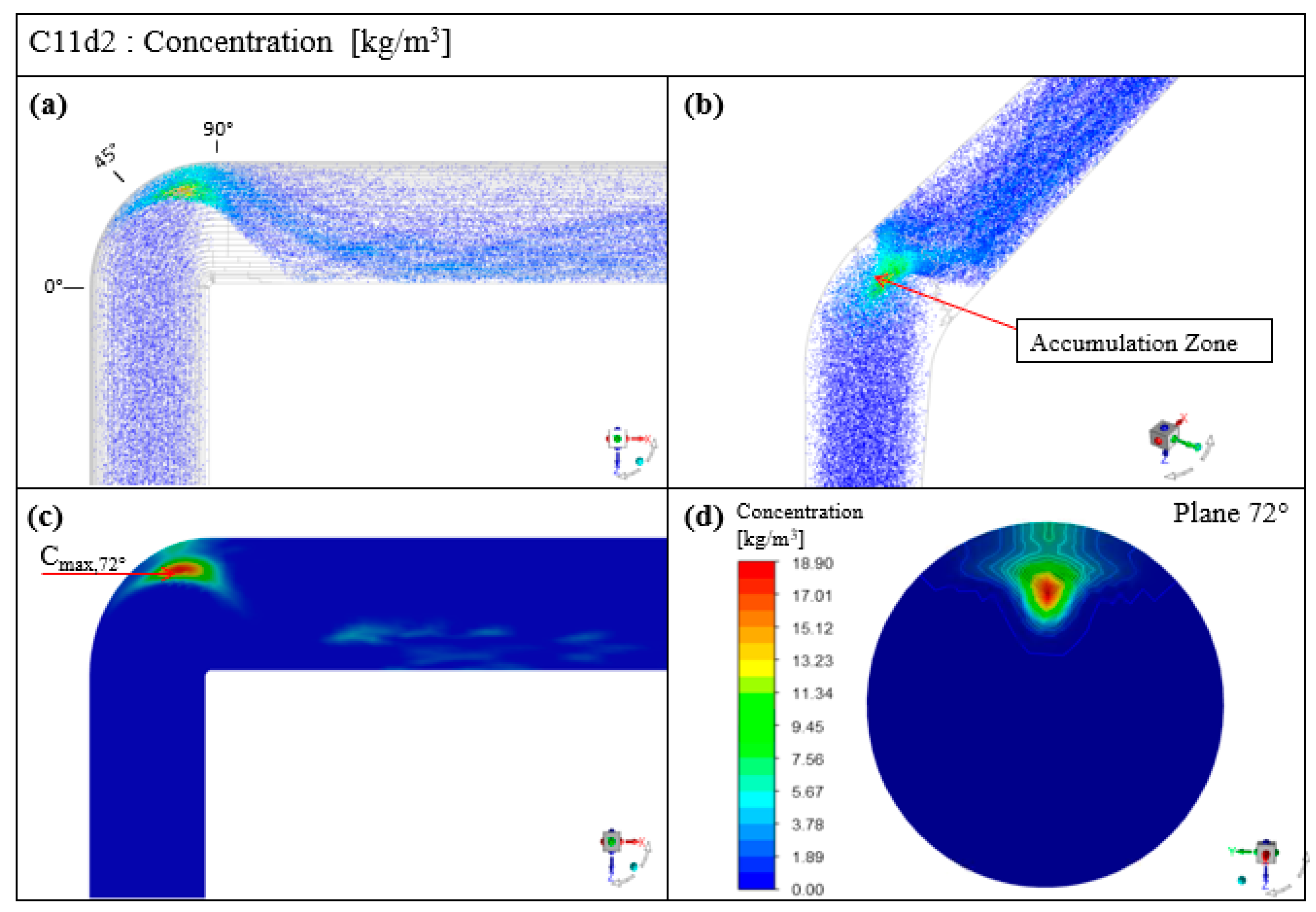
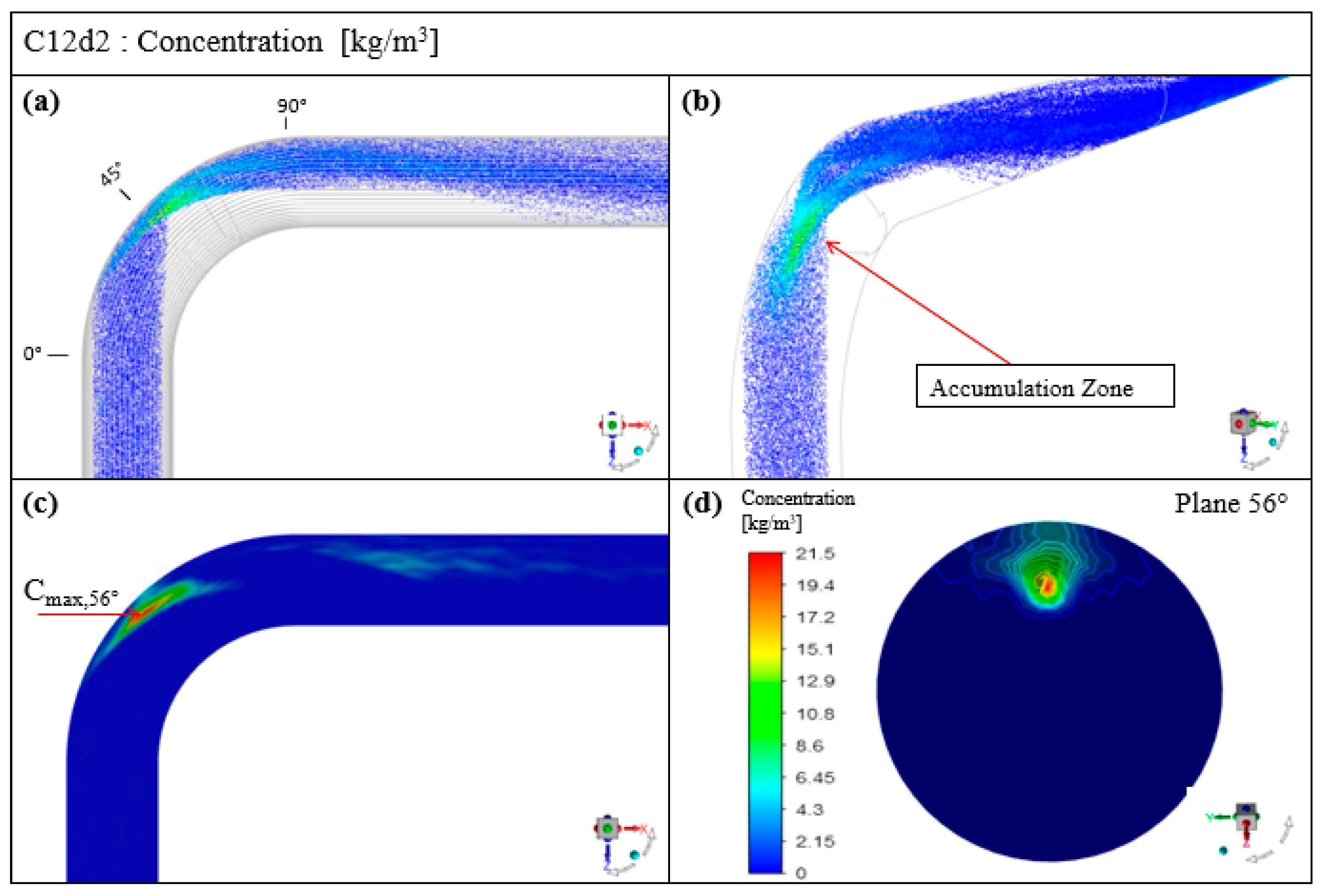
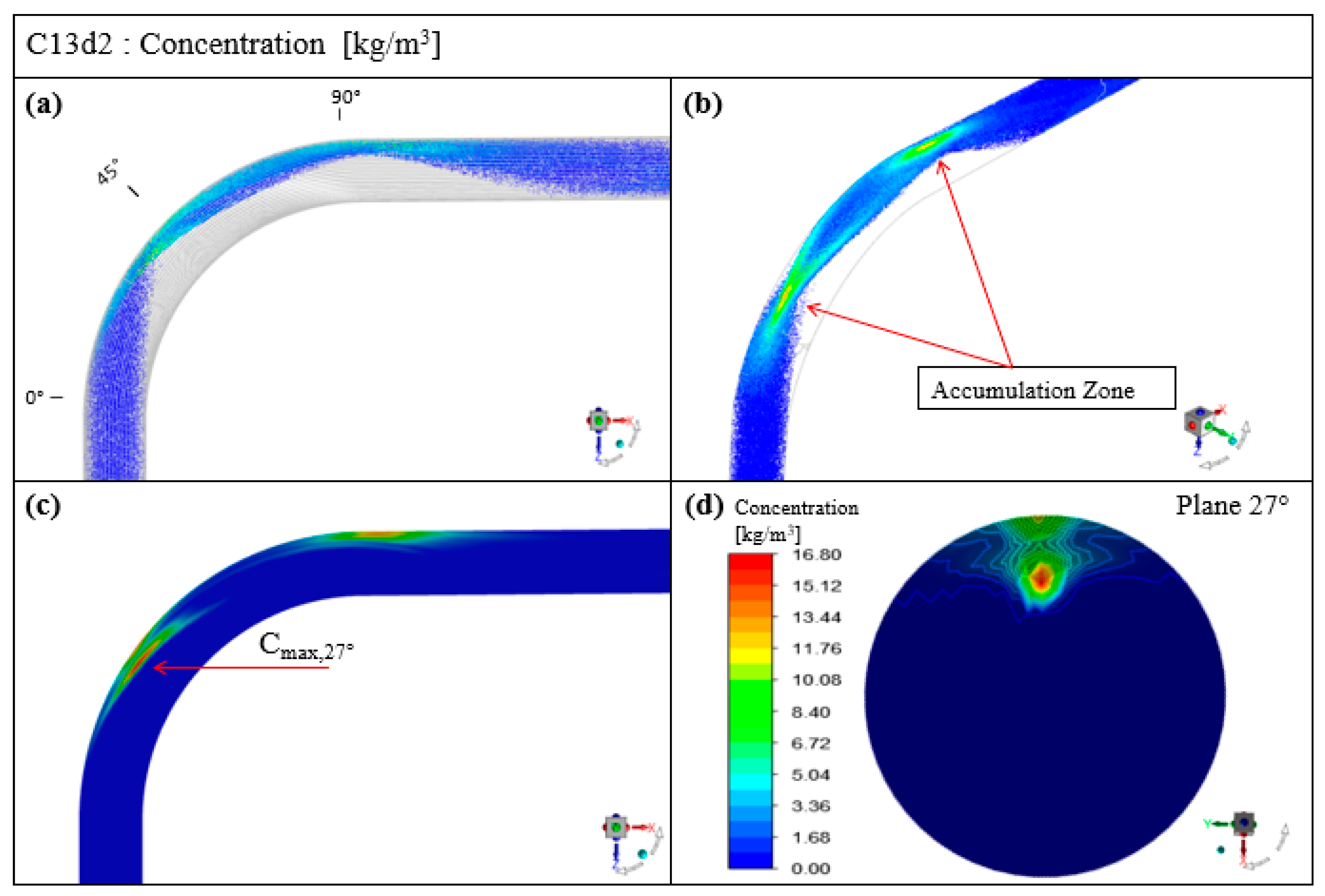
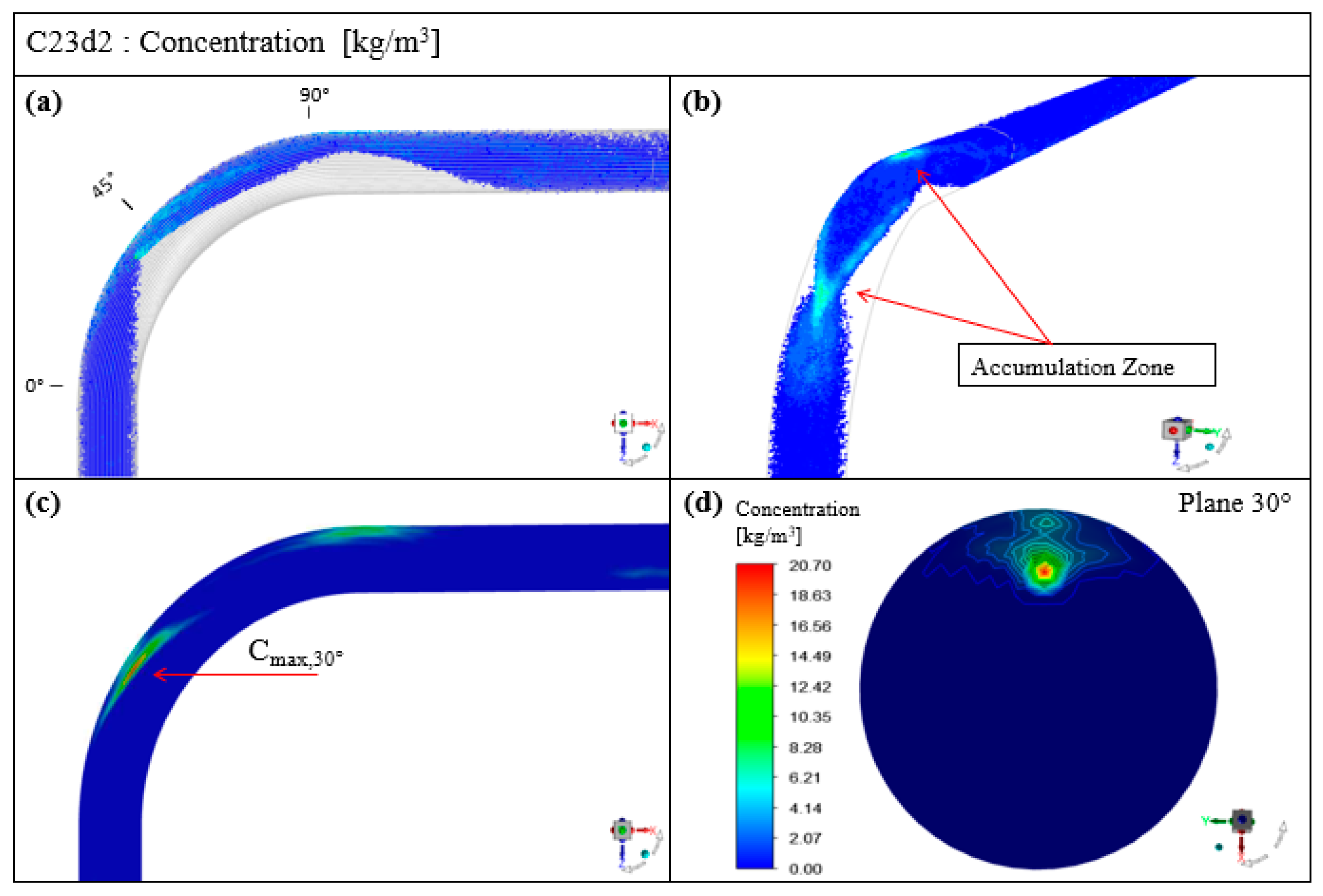
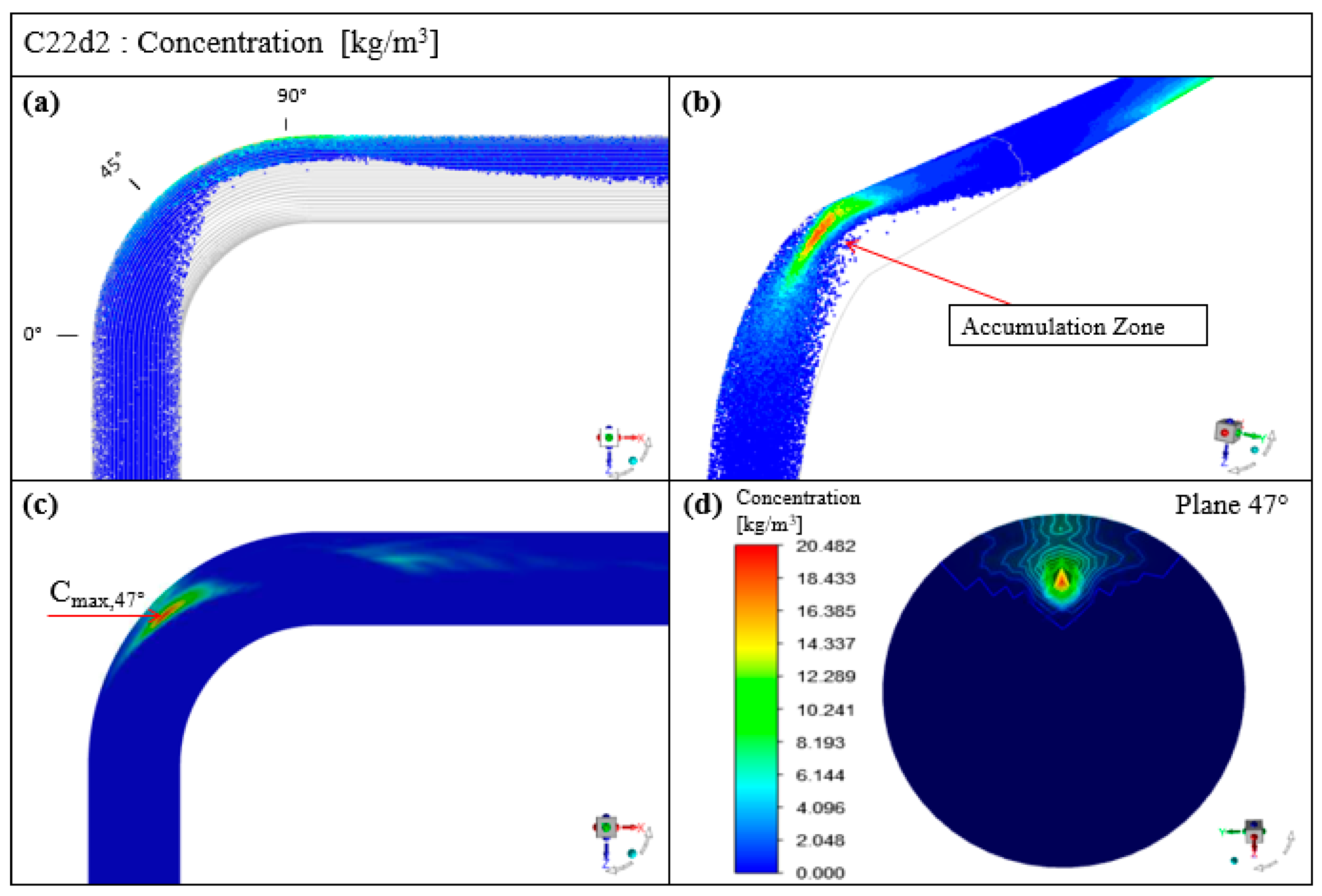
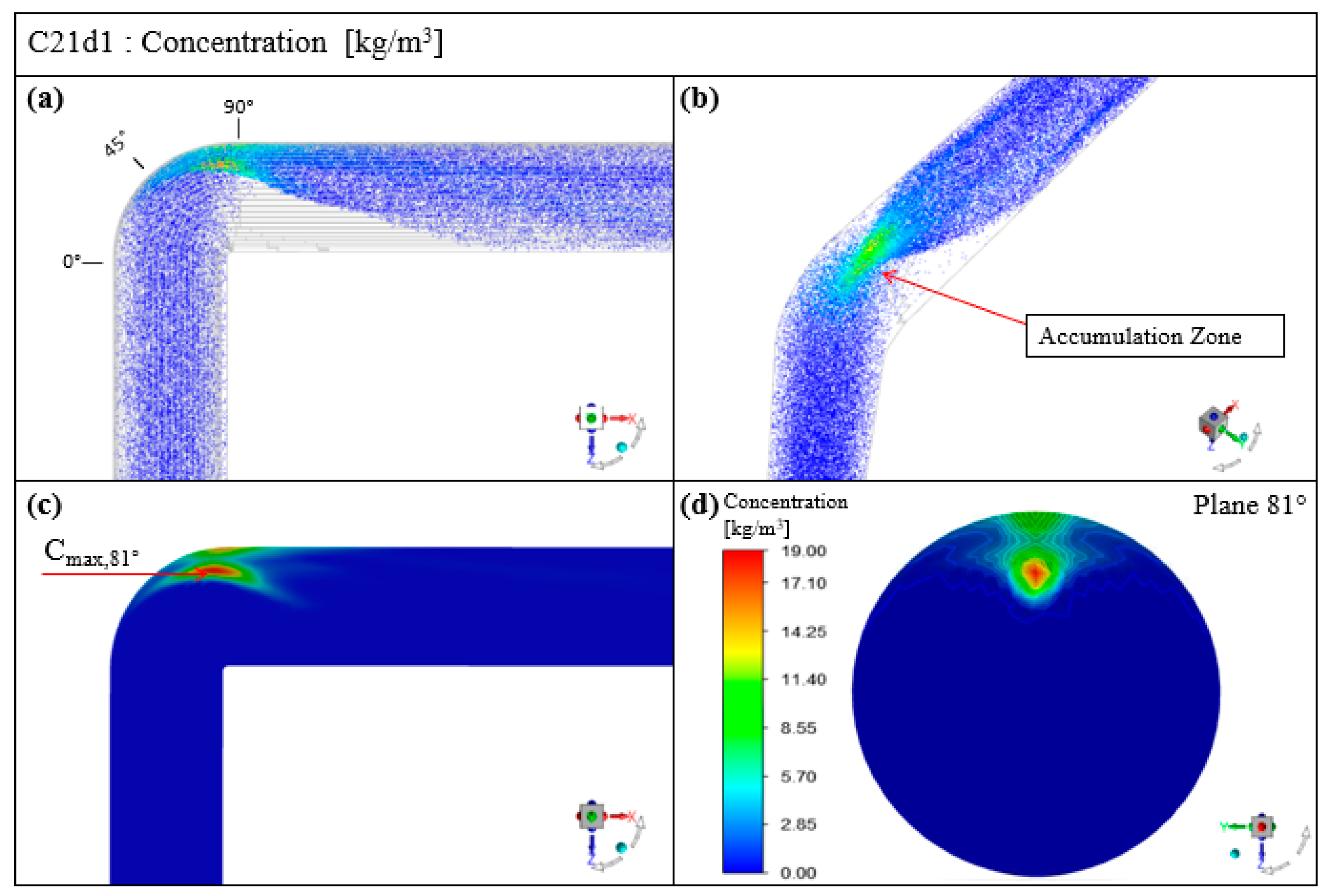
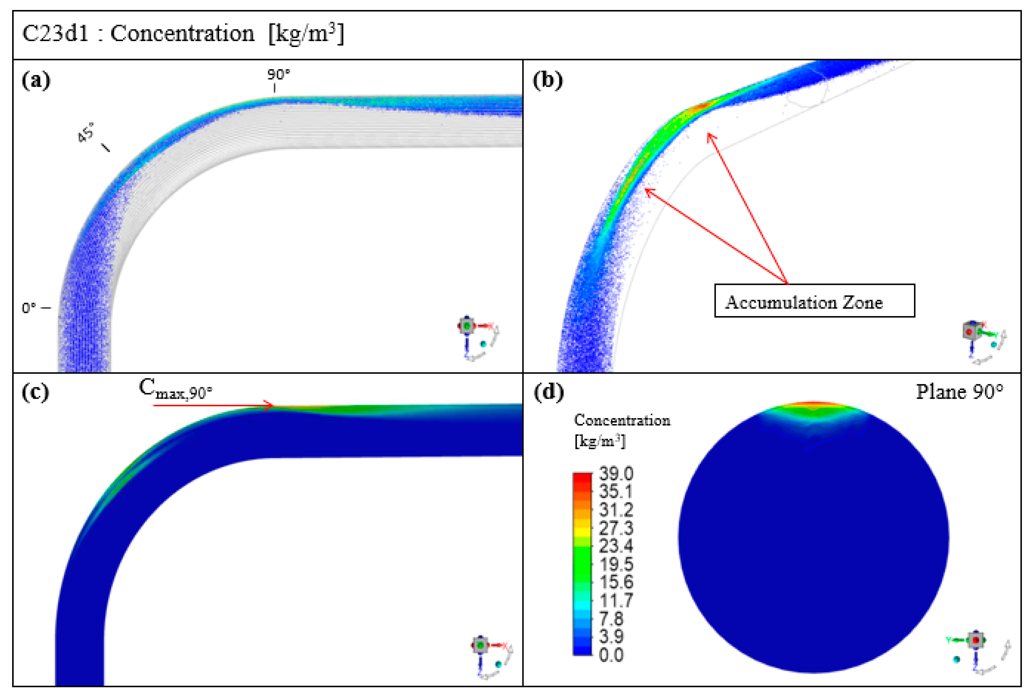
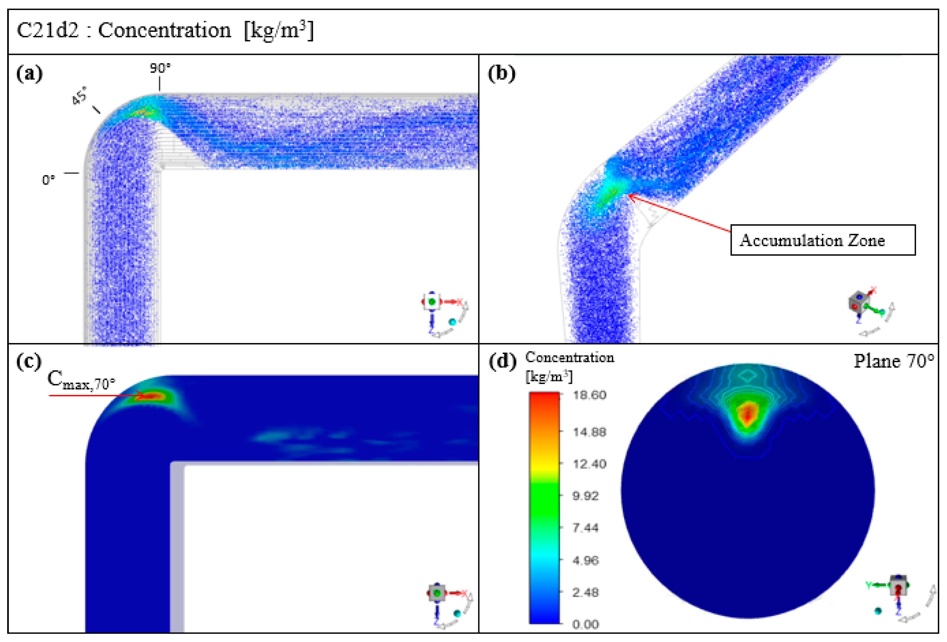
Figure 10 shows the concentration distribution along the curve. A maximum concentration at φ = 87° can be identified for C12d1, which responds to a maximum concentration that remains constant over time “C_max”, identifying a zone of particle accumulation. Figure 11 shows the concentration of the particles at φ = 87°. Figure 11a,b presents the instantaneous positioning (for a statistically stationary flow) of the particles in 3D view, evidencing the accumulation zone inside the bend. 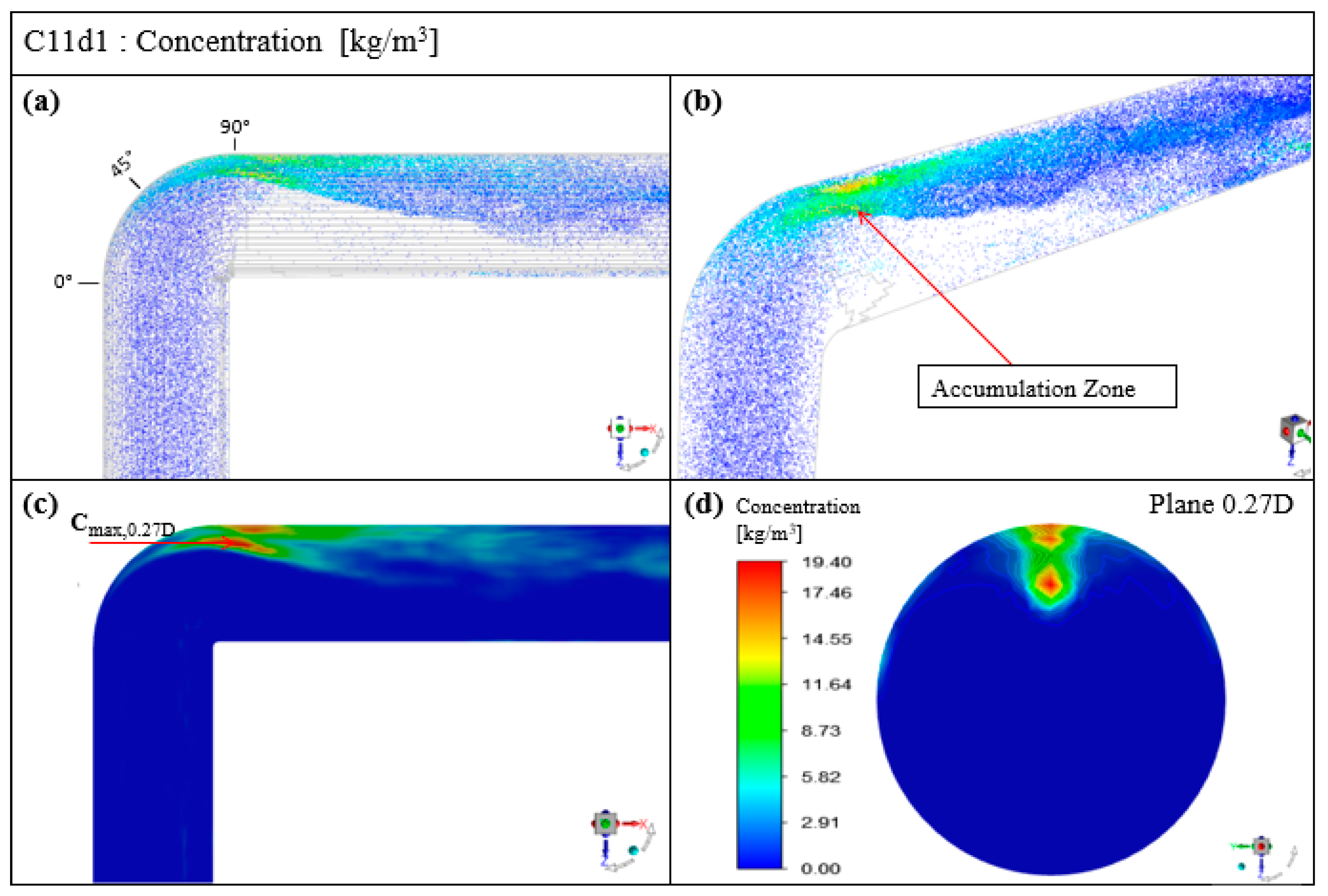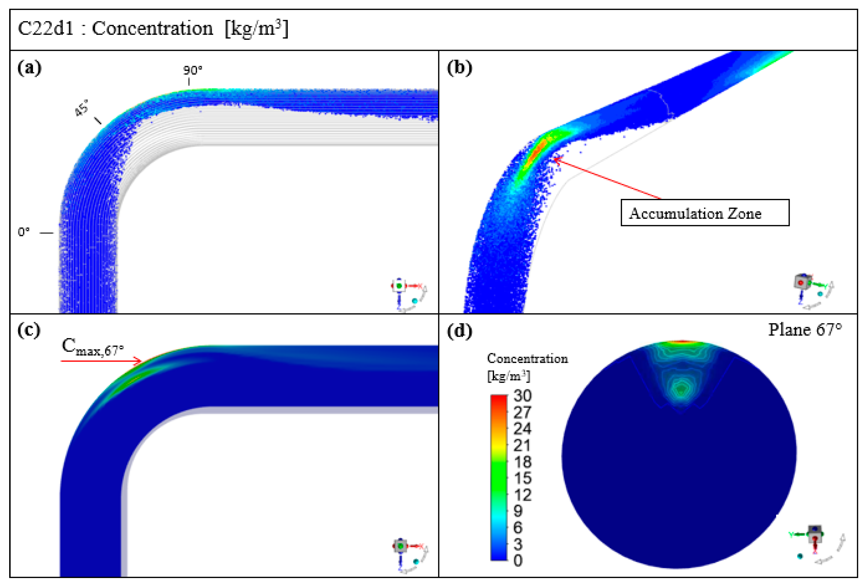Figure 11c,d shows, respectively, the concentration contour in the vertical mid-section plane of the pipe and the cross-section, demonstrating that the accumulation occurs towards the outside wall, in the longitudinal mid-section plane of the pipe. Another interesting aspect is that the position or location of the area of greatest accumulation within the elbow, although it occurs in the middle plane, is not completely defined in which deviation (φ) of the elbow it will occur. This is clear when comparing, in Figure 10, the C_max zone of the cases C13d1, C12d1, C11d1, since there is no important difference in the location of the maximum concentration between one and the other (90°, 87° and 0.25D of the bend, respectively), even though the Dean vortex formation point is near the inlet of the elbow for the case with the highest curvature ratio (C13d1) and practically at the exit for the lowest curvature ratio (C11d1). Similarly, if we compare the cases according to Re, no specific trend is noticeable regarding the concentration. However, when comparing equivalent cases, but using different particle sizes, for instance C13d1 and C13d2, it could be observed that, for larger particle size (dp), the accumulation point was delayed. On the other hand, this would not explain why the particles are focused on the mid-section plane and towards the outside wall of the pipe. A possible explanation could be that there is an accumulation mechanism related to the interaction between the secondary flow (vortices) and the inertial responsiveness of the particles to be centrifuged by it.

C_max is considered as a benchmark in our study in addition to the Stokes numbers for the prediction of the concentration or accumulation of particles within an elbow.

Table 6. Cases studied and their corresponding maximum concentration within the elbow.

Codification	C11d1	C12d1	C13d1	C21d1	C22d1	C23d1	C11d2	C12d2	C13d2	C21d2	C22d2	C23d2
Cmax [kg/m3]	19.4	45.8	201.5	19	30	39	18.9	22.1	16.8	18.6	20.5	20.7

summarizes the C_max of the 12 solved cases and

Table 7. Cases studied and their corresponding Stokes numbers.

	$\mathit{S}\mathit{t}{\mathit{k}}_{\mathit{c}\mathit{u}\mathit{r}\mathit{v}\mathit{e}\mathit{d}}$	$\mathit{S}\mathit{t}{\mathit{k}}_{{\mathit{t}}_{\mathit{r}}}$	$\mathit{S}\mathit{t}{\mathit{k}}_{{\mathit{w}}_{\mathit{c}}}$	$\mathit{S}\mathit{t}{\mathit{k}}_{{\mathit{w}}_{\mathit{v}}}$	C = Cmax/Cmax_C13d2
C11d1	0.11	0.45	0.29	0.55	1.15
C12d1	0.92	1.80	1.14	0.86	2.73
C13d1	1.87	3.60	13.23	1.46	11.99
C21d1	0.01	0.16	0.10	0.20	1.13
C22d1	0.10	0.64	0.40	0.34	1.79
C23d1	0.21	1.27	0.81	0.51	2.32
C11d2	0.04	0.05	0.03	0.06	1.12
C12d2	0.33	0.20	0.13	0.10	1.38
C13d2	0.68	0.40	0.25	0.16	1.00
C21d2	0.005	0.02	0.01	0.02	1.11
C22d2	0.04	0.07	0.04	0.04	1.22
C23d2	0.08	0.14	0.09	0.06	1.23

summarizes the values of the ad hoc formulated Stokes numbers together with the relative concentration (C), where the relative concentration is obtained by dimensioning the C_max of the selected case by the lowest C_max recorded among the solved cases, being C = C_max/C_{max_C13d2}.

Additional information on this topic is presented in Appendix B, including the values of the maximum velocity (

Table A1. Cases studied and their corresponding maximum concentration within the elbow.

Codification	C11d1	C12d1	C13d1	C21d1	C22d1	C23d1	C11d2	C12d2	C13d2	C21d2	C22d2	C23d2
Vmax [m/s]	21.9	10.8	10.7	66.4	30.3	29.2	24.4	10.9	10.5	70.7	30.4	29.3

) and maximum tangential velocity (

Table A2. Cases studied and their corresponding maximum concentration within the elbow.

Codification	C11d1	C12d1	C13d1	C21d1	C22d1	C23d1	C11d2	C12d2	C13d2	C21d2	C22d2	C23d2
Vtan.máx [m/s]	9	5.8	3.4	25.4	14.6	9.8	10	5.4	3.4	30	15.6	9.8

) obtained and used for the calculation of the Stokes numbers.

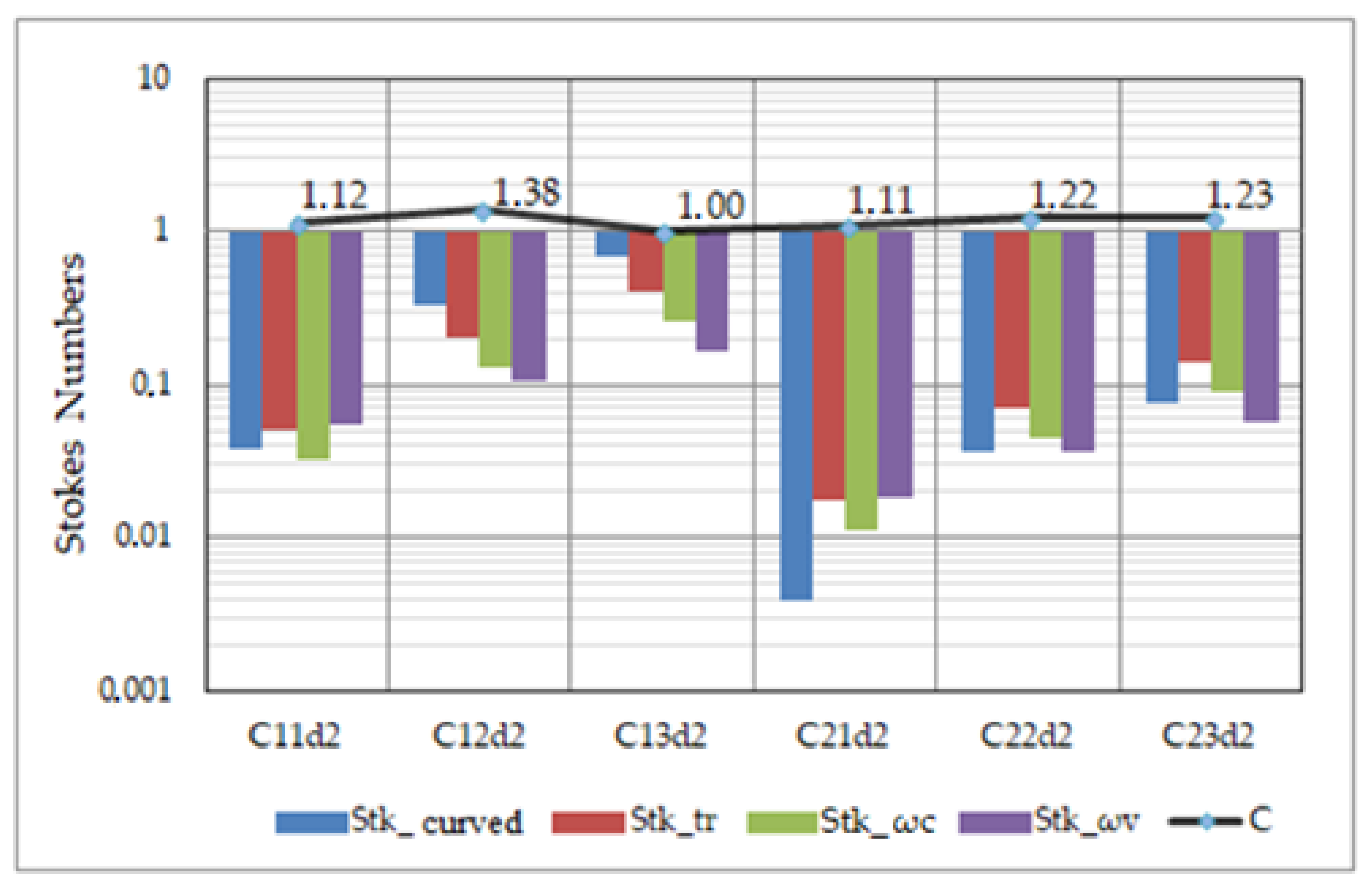
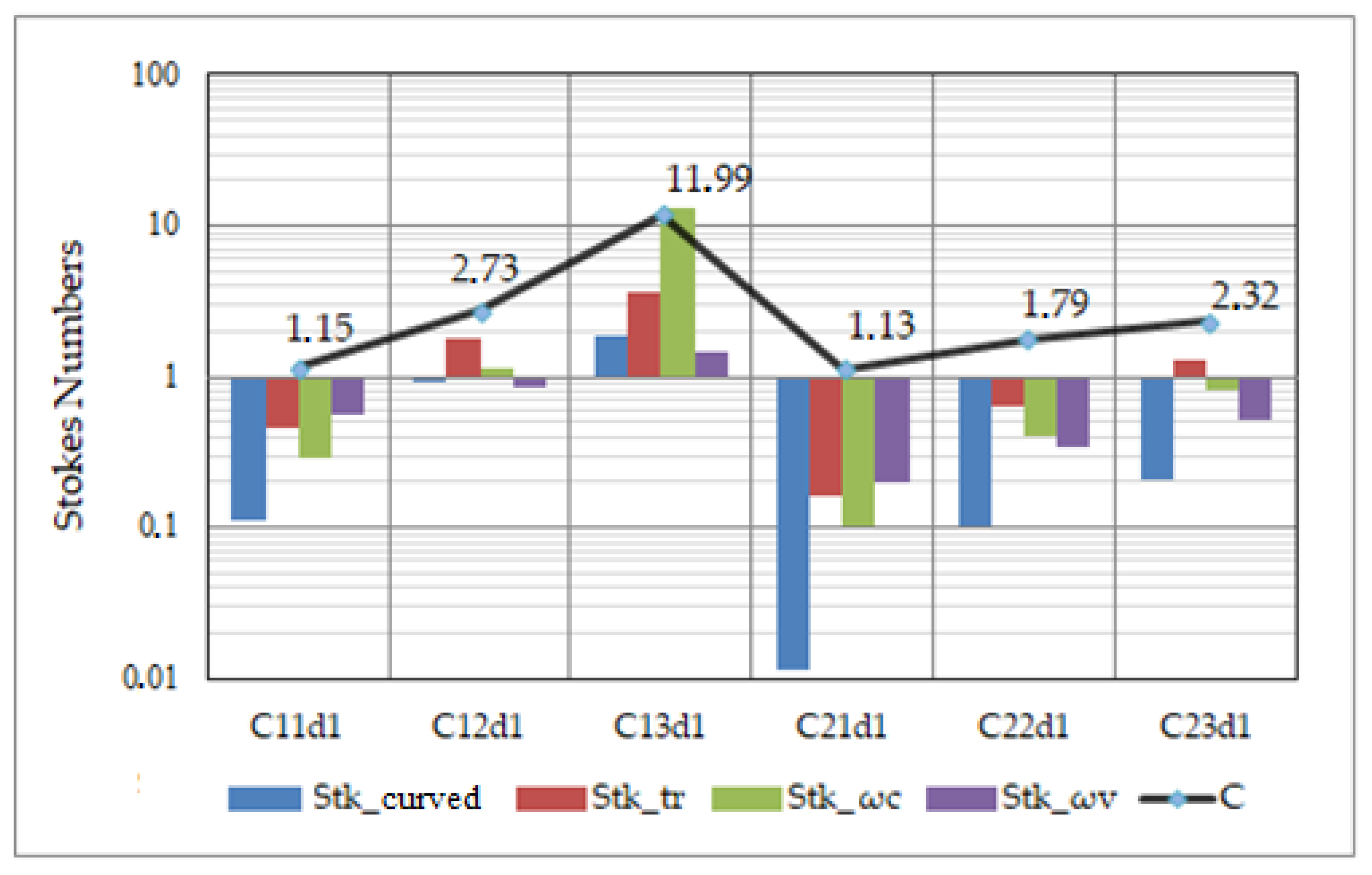
The inertial responsiveness of each particle size is critical in describing how the particles will be concentrated. Therefore, the results are grouped and compared for d1 and d2. Figure 12 and Figure 13 present a comparison of the different Stokes numbers for each case in addition to the value of the relative concentration. Overall, the four formulations of Stokes number mirror the accumulation process, with the four Stk showing the same overall trend as the concentration number.

Figure 12 shows that, in cases with particle size 50 µm (d1), the Stokes numbers qualitatively show a correlation between the increase of the four Stokes numbers and the relative concentration (i.e., the higher the value of the four Stokes numbers, the higher the underlying maximum concentration). Three scenarios can be identified: First, if $St{k}_{ curved},St{k}_{ t_r},St{k}_{ {\omega }_c}, St{k}_{ {\omega }_v}>1$, then the maximum relative concentration was reached (C = 11.99); in the same way, if $St{k}_{ curved}, St{k}_{ t_r}, St{k}_{ {\omega }_c},St{k}_{ {\omega }_v}<1$, then the minimum concentration levels were observed; finally, when $St{k}_{ curved},St{k}_{ {\omega }_c}, St{k}_{ {\omega }_v}$ were close to 1 and $St{k}_{ t_r}>1$, an increase in concentration is noticeable.

Although Stokes numbers are intended to predict the increase in particle concentration, it should be noted that a higher accumulation occurs at a higher curvature ratio (compare C11d1→C13d1; C21d1→C23d1), at a lower Reynolds number (C11d1/C21d1; C12d1/C22d1; C13d1/C23d1) and smaller particle size (see Figure 12 and Figure 13).

In Figure 13, the cases with particle size 150 µm (d2) show a different pattern: The case C13d2 had the lowest C_max recorded with 16.8 kg/m³ and subsequently C = 1, in contrast to the cases with particle size 50 µm (d1).

Overall, a similar maximum concentration is achieved in all cases, with C12d2 showing the highest relative concentration (C = 1.38). It can also be observed that $St{k}_{ curved}, St{k}_{ t_r}, St{k}_{ {\omega }_c}, St{k}_{ {\omega }_v}<1$ is simultaneously fulfilled for relative minimum concentration levels as with the cases C11d1, C21d1 and C22d1, much like in the cases with particle size 50 µm (d1) shown in Figure 12. While a greater curvature ratio, a lower Reynolds number and smaller particle size promotes accumulation (Figure 12), a larger particle size minimizes the effect of these parameters on the accumulation.

As the particle grows, it is practically unaffected by the vortices due to the inertia to overcome to be centrifuged by the secondary flow. A confirmation that this could be the reason is verified in the case of C11d1, which, despite being smaller in size, presents a concentration similar to the cases with particle size d2. This is due to the fact that, in the minimum theoretically possible curvature ratio “R/Rc = 1”, the vortices are formed at the exit of the curve (at 0.25 D), reducing the accumulation effect produced by the secondary flow, and its inertia dominating the trajectory of the particles.

4. Conclusions

In this work we address the problem of quantifying, by means of ad hoc Stokes numbers, the accumulation of solid particles carried by a turbulent air flow inside a 90° bend pipes. Average and maximum flow velocity statistics were obtained, in addition to other parameters, such as angular velocity and maximum tangential velocity inside the bend. An effective way to study the accumulation inside the bend was presented through the results of concentration and distribution of particles inside the pipe, under the premise that, if there is an increase in concentration over time, it reveals particle accumulation. The simulation captured the secondary flow statistics of two three-dimensional counter-rotating vortices covering the entire cross section of the pipe, also known as dean vortices, which are caused by the unbalance between the adverse pressure generated and the velocity field of the flow, characterizing the flow in a curved pipe.

Different flow configurations (Reynolds numbers, particle sizes and curvature ratios) were studied. The fluid and particle velocity statistics were adequately resolved in all cases, observing that the secondary flow acts as the main particle accumulation mechanism acting as a particle centrifuge, where a lesser effect of the counter-rotating vortices leads to a decrease in particle concentration. Although the accumulation cannot be eliminated for high Dean numbers due to the presence of the vortices, in fact the parameters studied can be manipulated depending on the application to achieve a minimum level of concentration even with a strong secondary flow present. The most important parameters to take into account are the lowest possible radius of curvature, but always in combination with a relatively small number of deans in order to keep the angular velocity of the eddies low. Following these steps, it would be possible to keep a low Stokes number, thus controlling the concentration within the elbow. It should be noted that, having used a URANS modelling, there are scales and turbulent structures not considered, so that a study using a DNS could identify other factors that could play a role in the accumulation in addition to the influence of the size of the particles and the mechanism of accumulation of large scale Dean vortices.

Finally, regarding the different Stokes numbers $(St{k}_{ curved}, St{k}_{ t_r}, St{k}_{ {\omega }_c}, St{k}_{ {\omega }_v}$), it was observed that simultaneous values greater than one were linked to a noticeable increase of the maximum concentration inside the pipe bend. Likewise, for simultaneous values of Stokes numbers less than one, a minimum of relative concentration is present. In addition, there is a correlation between the Stokes value with intermediate levels of concentration as Stokes numbers increase for values of $St{k}_{ curved}, St{k}_{ {\omega }_c}, St{k}_{ {\omega }_v}$ close to the unity and $St{k}_{ t_r}$ > 1, the latter being the one that apparently presents the greatest correlation force.

References

1. McFarland, A.R.; Gong, H.; Muyshondt, A.; Wente, W.B.; Anand, N.K. Aerosol Deposition in Bends with Turbulent Flow. Environ. Sci. Technol. 1997, 31, 3371–3377. [Google Scholar] [CrossRef]
2. Breuer, M.; Baytekin, H.T.; Matida, E.A. Prediction of Aerosol Deposition in 90∘ Bends Using LES and an Efficient Lagrangian Tracking Method. J. Aerosol Sci. 2006, 37, 1407–1428. [Google Scholar] [CrossRef]
3. Pui, D.Y.H.; Romay-Novas, F.; Liu, B.Y.H. Experimental Study of Particle Deposition in Bends of Circular Cross Section. Aerosol Sci. Technol. 1987, 7, 301–315. [Google Scholar] [CrossRef]
4. Zhang, P.; Roberts, R.M.; Bénard, A. Computational Guidelines and an Empirical Model for Particle Deposition in Curved Pipes Using an Eulerian-Lagrangian Approach. J. Aerosol Sci. 2012, 53, 1–20. [Google Scholar] [CrossRef]
5. Noorani, A.; Sardina, G.; Brandt, L.; Schlatter, P. Particle Transport in Turbulent Curved Pipe Flow. J. Fluid Mech. 2016, 793, 248–279. [Google Scholar] [CrossRef] [Green Version]
6. Guda, S.S.; Rowan, S.L.; Yang, T.; Shaffer, F.; Celik, I.B. Investigation of Rope Formation in Gas–Solid Flows through a 90° Pipe Bend Using High-Speed Video and CFD Simulations. J. Comput. Multiph. Flows 2018, 10, 3–18. [Google Scholar] [CrossRef]
7. Torras, S.; Torres, M.; Escalante, H.; Rosales, W. Simulación Computacional de la Hidrodinámica Del, Flujo. Rev. Cient. Unet 2006, 18, 212–216. [Google Scholar]
8. Kim, J.; Yadav, M.; Kim, S. Characteristics of Secondary Flow Induced by 90-Degree Elbow in Turbulent Pipe Flow. Eng. Appl. Comput. Fluid Mech. 2014, 8, 229–239. [Google Scholar] [CrossRef]
9. Maxey, M.R.; Riley, J.J. Equation of Motion for a Small Rigid Sphere in a Nonuniform Flow. Phys. Fluids 1983, 26, 883–889. [Google Scholar] [CrossRef]
10. Sudo, K.; Sumida, M.; Hibara, H. Experimental Investigation on Turbulent Flow in a Circular-Sectioned 90-Degree Bend. Exp. Fluids 1998, 25, 42–49. [Google Scholar] [CrossRef]
11. Kalpakli, A. Experimental Study of Turbulent Flows through Pipe Bends. Ph.D. Thesis, KTH Royal Institute of Technology, Stockholm, Sweden, 2012. [Google Scholar]
12. Hinze, J.O. Turbulent Fluid and Particle Interaction. In Proceedings of the International Symposium on Two-Phase Systems; Hetsroni, G., Sideman, S., Hartnett, J.P., Eds.; Pergamon: Oxford, UK, 1972; pp. 433–452. ISBN 978-0-08-017035-0. [Google Scholar]
13. Sommerfeld, M. Theoretical and Experimental Modelling of Particulate Flow von Karman Institute. Available online: https://store.vki.ac.be/theoretical-and-experimental-modelling-of-particulate-flow.html (accessed on 15 March 2021).
Figure 1. Definition of the geometric parameters in the models.
Applsci 11 07381 g001
Figure 2. Comparison between experimental (markers) and estimated (lines) pressure drop values using different models. The experimental values, RSM model and k-ε are those reported by Zhang et al. [4].
Applsci 11 07381 g002
Figure 3. Longitudinal flow velocity comparisons at z/D = 0, z/D = 1, z/D = 2, z/D = 3.5, z/D = 10 and z/D = 50. (a) Vertical plane (θ = 90°); (b) horizontal plane (θ = 0°). Solid line: RNG k-ε turbulence model results. Experimental data from Sudo et al. (Re = 60,000) [10] and Kim et al. (Re = 50,800) [8].
Applsci 11 07381 g003aApplsci 11 07381 g003b
Figure 4. Flow velocities in cross section z/D = −1, φ = 0°, φ = 30°, φ = 60°, φ = 90°, z/D = 2 and z/D = 10. Figures above in color represent the results obtained with the RNG k-ε model, where the numerical values are normalized by the axial velocity of the flow, W ¯ / Wa . The lower figures (in black) are the velocity contours given [10]. For each figure, the left side represents the inner area of the curve and the right side the outer area.
Applsci 11 07381 g004aApplsci 11 07381 g004b
Figure 5. Particle concentration profiles in vertical symmetric lines in “y” (θ = 90 °) for z/D = 0.25, z/D =1, z/D =2. Load condition (a) 35% and (b) 45%. Experimentally computed values (line marker) [6] and estimated with RNG k-ε model (line only).
Applsci 11 07381 g005aApplsci 11 07381 g005b
Figure 6. Longitudinal flow velocity profile in z’/D = −1, φ = 0°, 30°, 45°, 60° and 90°. RNG k-ε model. Experimental data of Sudo et al. (Re = 60,000) [10].
Applsci 11 07381 g006
Figure 7. Coding of study case.
Applsci 11 07381 g007
Figure 8. Geometrical models generated in ANSYS SpaceClaim. (a) Rc/R = 1; (b) Rc/R = 4; (c) Rc/R = 8.
Applsci 11 07381 g008
Figure 9. Example of mesh case C22. (a) Axial direction, middle plane; (b) radial direction, pipe entry.
Applsci 11 07381 g009
Figure 10. Maximum distribution of concentration in the medial plane of the elbow. Of the cases C11d1, C12d1 (reference case) and C13d1.
Applsci 11 07381 g010
Figure 11. Results of particle concentration. Reference Case C12d1. (a) Instant positioning of the X-Z plane particles (b) Instant positioning of the particles in 3D view (c) Concentration contour in the X-Z plane of the mid-section of the pipe (d) Concentration contour in the Z-Y plane of the maximum concentration cross section. Snapshots are taken for a statistically steady flow.
Applsci 11 07381 g011
Figure 12. Bar graph of the Stokes numbers and trend line of relative concentrations between cases, for particle sizes d1 = 50 [μm].
Applsci 11 07381 g012
Figure 13. Bar graph of the Stokes numbers and trend line of relative concentrations between cases, for particle sizes d2 = 150 [μm].
Applsci 11 07381 g013