Evaluation of the Erosion Characteristics for a Marine Pump Using 3D RANS Simulations

Abstract

In the present study, an erosion analysis of an industrial pump’s casing and impeller blades has been performed computationally. Effects of various critical parameters, i.e., the concentration and size of solid particles, exit pressure head, and cavitation on the erosion rate density of the casing and blade have been investigated. Commercial codes CFX, ICEM-CFD, and ANSYS Turbogrid are employed to solve the model, mesh generation for the casing, and mesh generation of the impeller, respectively. The Eulerian-Eulerian method is employed to model the pump domain’s flow to solve the two phases (water and solid particles) and the interaction between the phases. Published experimental data was utilized to validate the employed computational model. Later, a parametric study was conducted to evaluate the effects of the parameters mentioned above on the erosion characteristics of the pump’s casing and impeller’s blade. The results show that the concentration of the solid particles significantly affects the pump’s erosion characteristics, followed by the particle size and distribution of the particle size. On the other hand, the exit pressure head and cavitation do not affect the erosion rates considerably but significantly influence the regions of high erosion rate densities.

1. Introduction

Centrifugal pumps are broadly employed in the process industries (e.g., coal, metallurgical and chemical processes) to transport solid-liquid slurries. The two most frequent challenges encountered during the transportation of slurries are a decline in the performance of the pumps and erosion of the wetted surfaces [1]. The components most subjected to high erosion rates are the impeller, liners, and pump casing [2]. Along with all the modules mentioned above, pump casing is the element that receives the greatest damage from erosion. This leads to frequent replacements of the casing, making it the most expensive component of the pump’s assembly [3]. Impact and sliding of the solid particles along the wall are two major contributors to erosion while slurry flows through pumps [4,5]. The impact of the particle will be a major concern if slurries are sufficiently dilute [6]. Moreover, it will be multidirectional in case of turbulent flow.

Numerous techniques have been utilized in the literature to assess erosion rates in the centrifugal pumps computationally. Employed computational methods in the literature are based on two-dimensional models, three-dimensional models, and a component-by-component approach. Methods utilizing 2D geometrical models have been employed by [7,8] to assess the erosion trends in the casing of the centrifugal pump. In this methodology, however, the viscous force term is overlooked. Moreover, particles with a size greater than 1 mm stimulate unpredictably in the solution.

Consequently, this technique limits the analysis to small particles. Pagalthivarthi et al. [9] used 3D RANS simulations to calculate the erosion wear in the casing of a dilute slurry flow. The prospective interpretation was used by Zhong and Minemura [10] to solve the transport phase. They resolved particle speeds by weighing the forces employing the Lagrangian approach. Addie et al. [11] applied finite element calculations to forecast the erosion characteristics based on RANS solutions. They discovered that their results were in close agreement with the particle image velocimetry (PIV) results of Charoenngam et al. [12].

The prediction of wear and tear in centrifugal pump casing is a complex phenomenon that depends on many parameters such as particle velocity, particle impact angle, turbulence flow field, surface texture, and inlet flow conditions. Many of these parameters depend on the geometry of the specific pump design; thus, predictions made for one particular pump do not apply to other pump geometries.

It can be deducted from the literature review that the working life of the pump’s casing can be determined by examining the collective effects of erosion characteristics on the component using experimental or numerical methods. Experimental procedures are incredibly costly and time-exhausting. Therefore, in the current work, erosion characteristics associated with the pump’s impeller and the casing are evaluated by employing 3D RANS simulations. A parametric study based on four parameters, i.e., the concentration of solid particles, size of the solid particles, exit head, and cavitation, has been conducted. A set of commercial codes ANSYS-CFX, ICEM CFD, and turbo grid in an environment of the ANSYS workbench are employed to resolve the 3D RANS using the Eulerian-Eulerian method. The shear stress turbulence model (SST) is implemented to achieve better accuracy in the rotating domain of the impeller.

2. Computational Model

2.1. Governing Equations

As explained in the introduction section, a numerical study has been conducted to assess the influence of various factors, i.e., particle’s volume concentration (${\mathrm{P}}_{\mathrm{vc}}$), particle’s size (${\mathrm{P}}_{\mathrm{s}}$) and pump’s exit pressure (P_exit), on the erosion rate characteristics of the pump blade and its casing based on the Reynolds-averaged Navier-Stokes equations (RANS) calculations. The steady form of the employed transport equations, i.e., continuity, and momentum, was solved for both phases (water and sand). The two-phase numerical model was built using the Eulerian approach that is provided below using Equations (1)–(4) [13].

Continuity Equation for solid and fluid phase

$$\mathbf{\nabla }.\left(C_f{\rho }_f V_f\right)=0$$

(1)

$$\mathbf{\nabla }.\left(C_s{\rho }_s V_s\right)=0$$

(2)

Transport equations for solid and fluid phase

$$\mathbf{\nabla }.\left(C_f {\rho }_f{V}_f V_f \right)=-C_f 𝛻P+\mathbf{\nabla }.(C_f{\tau }_f)+C_f{\rho }_{f }g+R+C_f{\rho }_{f }\left(F_f+F_{l,f}+F_{v{m}_f}\right)$$

(3)

$$\mathbf{\nabla }.\left(C_s {\rho }_s{V}_s V_s \right)=-C_s 𝛻P+\mathbf{\nabla }.(C_s{\tau }_s)+C_s{\rho }_{s }g+R+C_f{\rho }_{f }\left(F_f+F_{l,s}+F_{vm,s}\right)$$

(4)

The terms, $V_f,{\tau }_f$ and $V_s,{\tau }_s$ denote flow velocity vector and shear stress tensor for both fluid and solid phases, respectively. On the other hand, the scalar quantities $C_f,C_s$ and ${\rho }_f,{\rho }_s$ are volume concentrations and densities of the fluid and solid phases, respectively. Force vector $R$ represents the interaction between the solid and liquid phases. While the term $P$ appearing in both Equations (3) and (4) represents the average pressure at the interfacial region of the two phases [14], and it is common for both fields. The lift force is represented by $F_l$, and $F_{vm,s}$ denotes the virtual mass force per unit mass. The lift force for solid phase $F_{l,S}$ can be calculated utilizing Equation (5) since: $F_{l,S}=-F_{l,f}$.

$$F_l,s=-0.5 C_s\left({\mathit{V}}_{\mathit{f}}-{\mathit{V}}_{\mathit{s}}\right)\times \left(\nabla .{\mathit{V}}_{\mathit{f}}\right)$$

(5)

Virtual mass force $F_{vm,s}$ is triggered by the acceleration of the solid phase through the fluid phase, and it was computed employing Equation (6).

$$F_{vm,s}=0.5 C_f{\rho }_f\left(\frac{d_f}{dt}\left(V_f\right)-\frac{d_s}{dt}\left(V_s\right)\right)$$

(6)

For coupling of both fields, i.e., water and solid particles, two procedures have been implemented in literature [15], namely one-way coupled and two-way coupled, based on the value of $\beta$ provided in Equation (7). If $\beta$ is less than 0.14, one-way coupling is recommended, otherwise, two-way coupling techniques should be utilized.

$$\beta =\frac{C_s{\rho }_s}{C_f{\rho }_f}$$

(7)

The prediction of wear rate that occurs largely on the casing walls was the major objective of this study. Thus to compute the accurate values of wear rate density, predicting the boundary layer and capturing the recirculation regions near the wall region is crucial.

Along with the available Reynolds-averaged Navier–Stokes (RANS) turbulence models, there are two classifications of turbulence models that have been employed in the literature depending on how the boundary layer is considered in those models [16,17,18]. In the first category of the RANS model, the flow in the boundary layer is not computed. Nonetheless, a wall function is utilized to approximate the velocity profile, e.g., $k-ϵ$ turbulence model. The $k-ϵ$ turbulence model manages a set of two transport equations to solve the turbulence kinetic intensity and dissipation. Concurrently, turbulent viscosity is shaped as a product of turbulent velocity and turbulent length scale. The $k-ϵ$ turbulence model is predominantly economical computationally and effective in solving the turbulence in the core flow region. However, at the same time, it does not solve the boundary, rather it estimates it using the built-in wall functions.

Consequently, the $k-ϵ$ turbulence model is not appropriate for flows with the boundary layer separation, flows with sudden changes in the mean streamflow, flows in revolving fluids, and flows over curved surfaces. On the other hand, the shear stress turbulence (SST) model combines two models [19,20,21,22,23,24,25], i.e., $k-\omega$ and $k-ϵ$ turbulence models according to the distance from the wall. Wilcox $k-\omega$ is utilized to resolve the flow in the vicinity of the walls for accurate prognostication of the boundary layer, whereas the $k-ϵ$ turbulence model is solving the flow in fully developed regions to gain advantage from its robustness, economy, and free stream independence [13,19]. Therefore, the shear stress turbulence (SST) model accounts for the transport of turbulent shear stress and avoids over-prediction of eddy viscosity. Numerous researchers [26,27,28,29,30,31] have adopted the shear stress transport (SST) turbulence model established by Menter [19] and achieved accurate aerodynamic predictions of rotating machines and complex flows. Based on the above discussion, the SST turbulence model was adopted for the current work as the flow was rotating. The accurate prediction of the boundary layer is critical for the precise evaluations of erosion.

Thus, the turbulence model that does not resolve the boundary layer and uses wall functions instead will not determine the flow feature near the walls. Many researchers [31,32,33] in the literature have employed the shear stress transport model (SST model) [19] to predict the near-wall phenomenon accurately for rotating machines. Thus, $the SST k-\omega$ turbulance model was adopted in the current study for turbulenace modeling. Details on the model could be found in [19].

2.2. Erosion Model

Modeling of erosion in complex geometries such as the case with the current work becomes complicated. This is because erosion is a compound function of particle parameters (size, roughness, shape, etc.), local flow characteristics, and complex turbulent fields along with multiphase effects (e.g., erosion shield due to solid accumulation and the restraining development produced by the liquid film, cavitation) along with the influence of local cavities due to material removal and properties of wall material.

Referring to Hutchings [34], erosion rates are a function of particle velocity (V_p) and impact angle ($\gamma )$ and with reference to this they suggested a relationship that is given by Equation (8).

$$E=k{V}_p^n f\left(\gamma \right)$$

(8)

The term $E$ denotes dimensionless mass value removed by the erosion phenomenon, $V_p$ is the particle’s velocity, and $f\left(\gamma \right)$ is a function of the particle’s impact angle. At the same time, the value of $n$ for different metals ranges from 2.3 to 2.5. It is impossible to formulate a universal erosion model under various conditions, and there is always a need for experimental studies to improve the model’s parameters. For the current work, Finnie’s [35] model was adopted with n = 2. Based on Finnie’s work, Equation (8) could be written as given below.

$$E=k{V}_p^2 f\left(\gamma \right)$$

(9)

In Equation (9)

$$\begin{array}{c}f\left(\gamma \right)=\frac{1}{3}{\cos }^2\gamma if\tan \gamma >\frac{1}{3}\\ f\left(\gamma \right)=\sin 2\gamma -3{\sin }^2\gamma if\tan \gamma \le \frac{1}{3}\end{array}$$

(10)

2.3. Cavitation Model

To understand the effects of cavitation on erosion, the cavitation phenomenon for water was modeled in the current work employing a homogeneous model to keep computation costs in check. For the simulations involving cavitation, both domains were initialized with water fraction 1. The same conditions were imposed at the inlet of the impeller. Mass transfer of liquid to vapor and vice versa was computed employing the cavitation model specified in Equation (11).

$$\frac{\partial }{\partial t}\left(C_{f,v}.{\rho }_{f,v}\right)+\nabla \left(C_{f,v }{\rho }_{f,v}{v}_{f,v}\right)={\alpha }_e-{\alpha }_c$$

(11)

Here ${\alpha }_e \mathrm{and} {\alpha }_c$ are cavitation coefficients for evaporation and condensation. And these constants could be computed utilizing the simplified Rayleigh-Plesset equation [36].

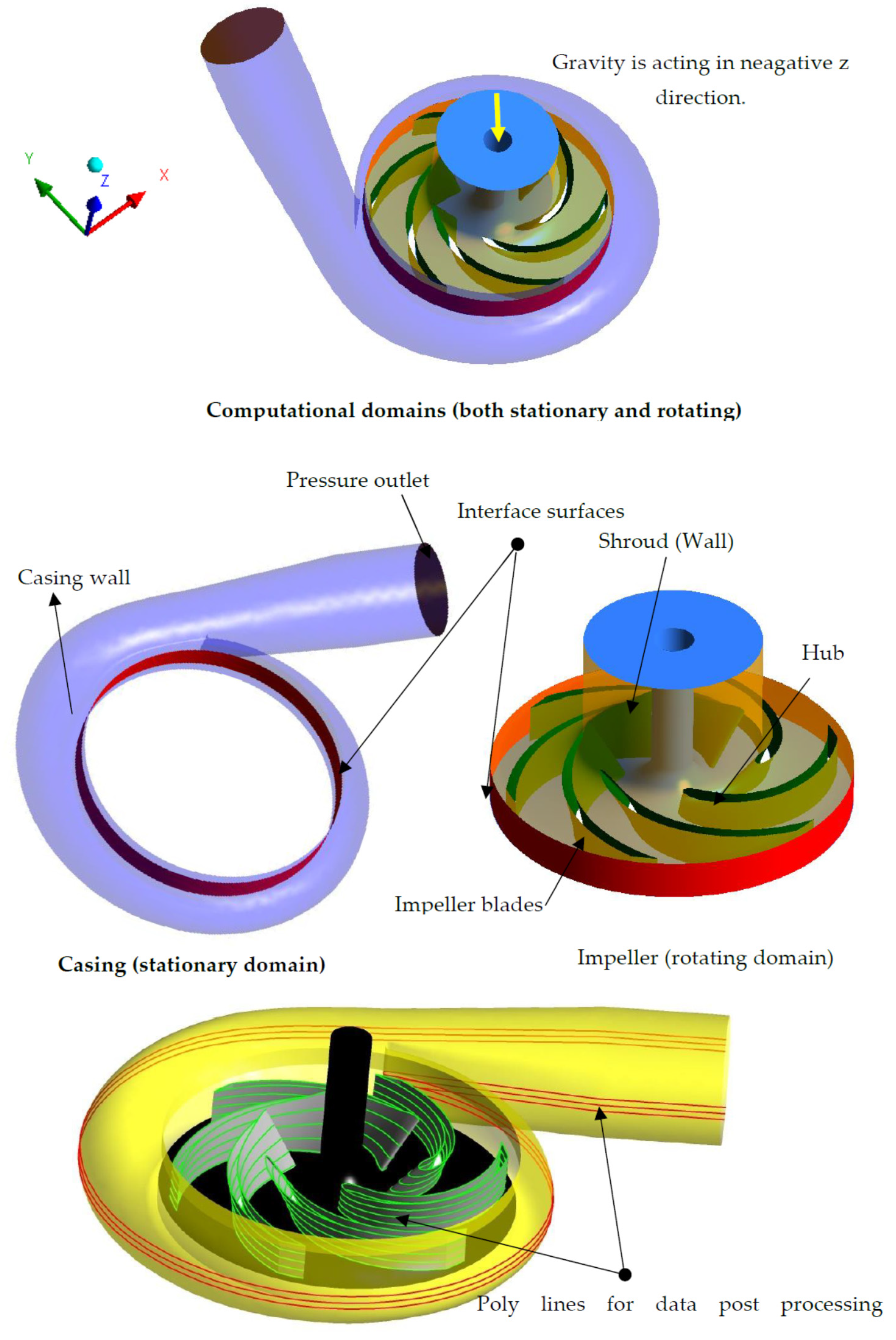
2.4. Computational Domain and Boundary Conditions

As referenced in the introduction section, the current study extended the author’s previous work that involved optimizing the pump’s geometry. Hence, the optimized geometry was utilized for the present study to report the impact of the particles’ concentration, size, pump exit pressure, and cavitation on the erosion of the pump’s blades and casing. The computational domain is shown in Figure 1, consisting of two sub-domains, i.e., the impeller (rotating at 1533 rpm) and the impeller’s casing (stationary). The interface between the rotating and stationary domains was modeled as a frozen rotor to mollify the conservation of all fluxes from impeller to casing. The inlet of the impeller was assigned with total inlet pressure and mass fractions of both phases. At the same time, static pressure was used at the exit of the casing.

The impact of the four parameters (solid particle’s concentration, size, pump exit pressure, and cavitation) was evaluated on the erosion characteristics of the pump’s impeller and pump’s casing. Five values each for the first three parameters (solid particle’s concentration, size, and pump exit pressure) were considered as listed in

Table 1. List of the simulations conducted for the current study.

Simulations	Exit Pressure ${\mathit{P}}_{\mathit{e}\mathit{x}\mathit{i}\mathit{t}} \left[\mathbf{bar}\right]$		Particle Concentration	Particle Distribution [$\mathsf{\mu }$m]
				Min	Min	Max	Ave	Std. Dev.
1	2.6, 2.7, 2.8, 2.9, 3.0	With cavitation and without cavitation	5%, 7.5%, 10%, 12.5%, 15%, 20%, 25%	Ps → A	50	250	150	120
				Ps → B	100	500	300	120
				Ps → C	150	750	450	120
				Ps → D	200	1000	600	120
				Ps → E	250	1250	750	120

. Finally, to study the impact of cavitation, the inlet pressure was adjusted to ensure that the pressure values within the pump dropped lower than the saturation pressure of the water. For this simulation, four values of the particle’s concentration, i.e., 5%, 7.5%, 10%, 12.5%, 15%, 20%, 25% were employed.

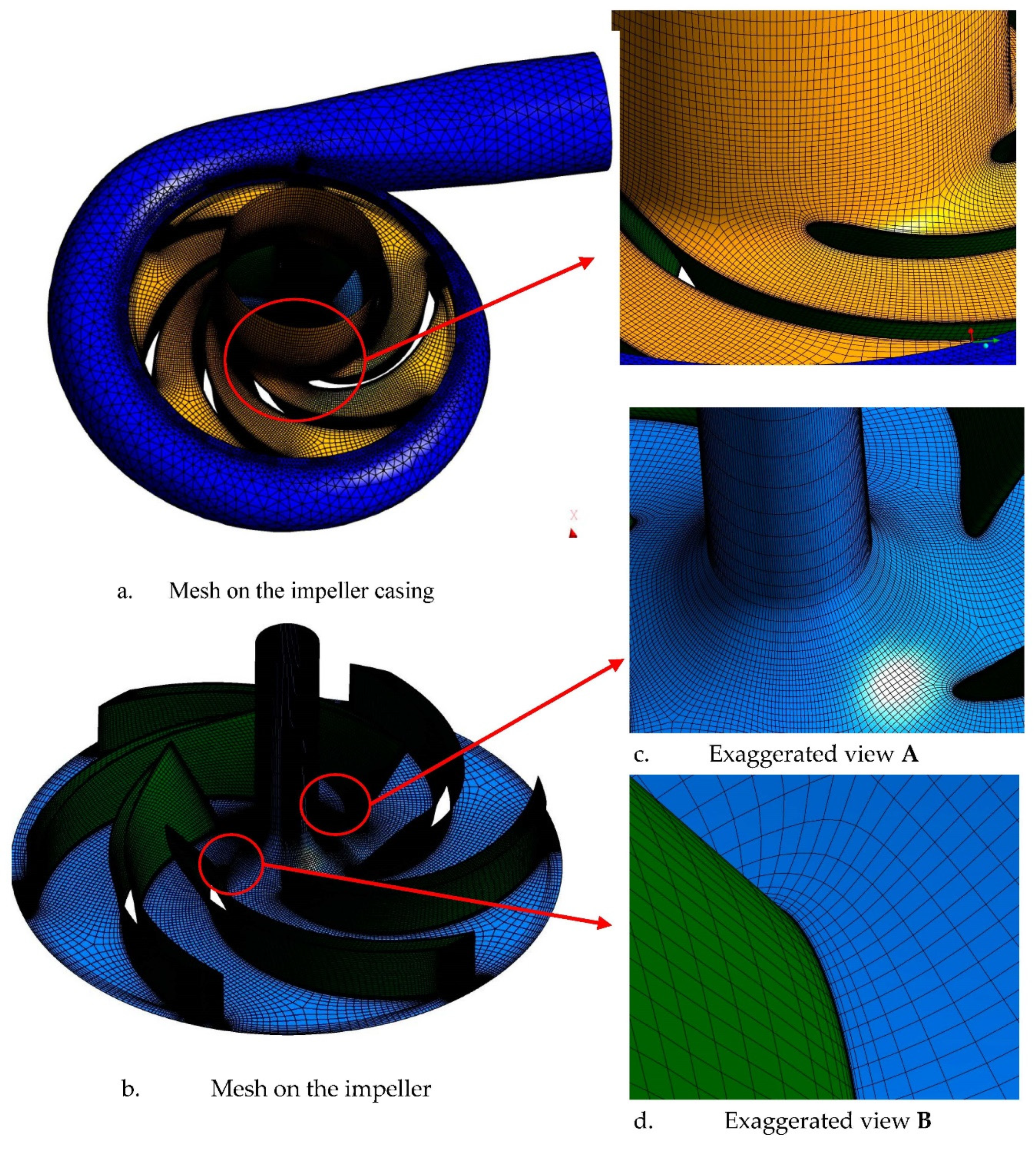
2.5. Mesh Generation

Two detached meshes were generated, one each for the impeller domain and the casing domain using different topologies, as shown in Figure 2. Structured mesh for the impeller’s domain using hexahedral elements was constructed. While unstructured mesh for the casing was generated using tetrahedral and prism elements, prism elements were only used in the prism layers near the wall for the flow in the boundary layer. To accomplish the requirements of the SST turbulence model, the value of ${\mathrm{y}}^{+}$ was guaranteed to be less than one for both stationary and rotating domains to acquire full advantage from the abilities of the SST turbulence model [19]. The ${\mathrm{y}}^{+}$ is a function of $\mathrm{\Delta }y$ (first node’s distance from the wall), flow length scale (L) and flow Reynolds number (Re). The value of $\mathrm{\Delta }y$ was calculated from Equation (12) to accomplish the desired value of ${\mathrm{y}}^{+}$ [37]. Further details on these calculations can be found in [30,38]. Mesh details are provided in

Table 2. Mesh details for the mesh optimization study.

	Rotating Domain (Impeller)				Stationary Domain (Casing)	Number of Nodes	Memory Allocate [MB]	Computation Time for Ten Iterations	Computed Pump Power [kW]
Mesh	Division along with the Blade Height	Divisions in the O-Grid Region	Divisions in the Tip Clearance Region	Divisions in the Inlet Domain	Element Size in the Stationary Domain
M1	35	10	5	15	0.003	1,025,341	11,325	57	11.2
M2	45	20	7	20	0.002	1,523,452	18,256	97	10.7
M3	60	30	11	25	0.0015	2,742,863	35,261	195	9.26
M4	70	40	15	30	0.001	3,929,536	47,325	310	9.19

.

$$\mathrm{\Delta }y=L y^{+}\sqrt{74} R{e}_L^{-\frac{13}{14}}$$

(12)

For accurate calculations, attaining only a desired ${ \mathrm{y}}^{+}$ value is not sufficient. Additionally, a minimum number of nodes $\left(n_{min}\right)$ within the boundary layer thickness $\left(\delta \right)$ are also required. For the SST turbulence model, the condition for $\left(n_{min}\right)$ is exemplified in Equation (13) [37].

$$\{\begin{array}{c}{y}_n\left(n_{min}\right) \le \delta \\ for SST n_{min }=15\\ y_n\left(15\right) \le \delta \end{array}$$

(13)

where $y_n\left(15\right)$ is the distance of node 15 from the wall.

The value of $\delta$ corresponding to $Re$ and $L$ was calculated from the following equation:

$$\delta =0.035 LR{e}_L^{-\frac{1}{7}}$$

(14)

The computed value of the boundary layer thickness was taken as equivalent to $y_n\left(n_{min}\right)$ and the mesh growth rate $\left(r_m\right)$ from the wall side was computed employing the geometric progression relation provided in Equation (16) to accomplish the desired value of the $n_{min}$ within the boundary layer thickness.

$$r_m={\left[\frac{ y_N\left(n_{min}\right)}{\mathrm{\Delta }y} \right]}^{\frac{1}{n_{min}-1}}$$

(15)

$$r_m={\left[\frac{ y_n\left(15\right)}{\mathrm{\Delta }y} \right]}^{1/14}$$

(16)

It is to be noted here that Equations (12) and (14) 4 were derived for a flat plate, but authors could not find any other method in the literature to adjust the value of y+. Therefore, in this work, Equations (12)–(14) were used to get an initial estimate of $\mathrm{\Delta }y$. Later an iterative process was used to achieve the required value of y+. The iterative process involved the following steps: (1) estimation of $\mathrm{\Delta }y$ from the equation node distribution in the boundary layer region; (2) updating the mesh based on the calculation in step; (3) solving the mesh in CFX; (4) postprocessing y+ from the obtained solution and finally adjusting the $\mathrm{\Delta }y$ values accordingly. The process mentioned above takes three to four iterations to achieve the required values of y+. Further, the chord length of the impellor’s blade was taken as the characteristic length “L” for these calculations

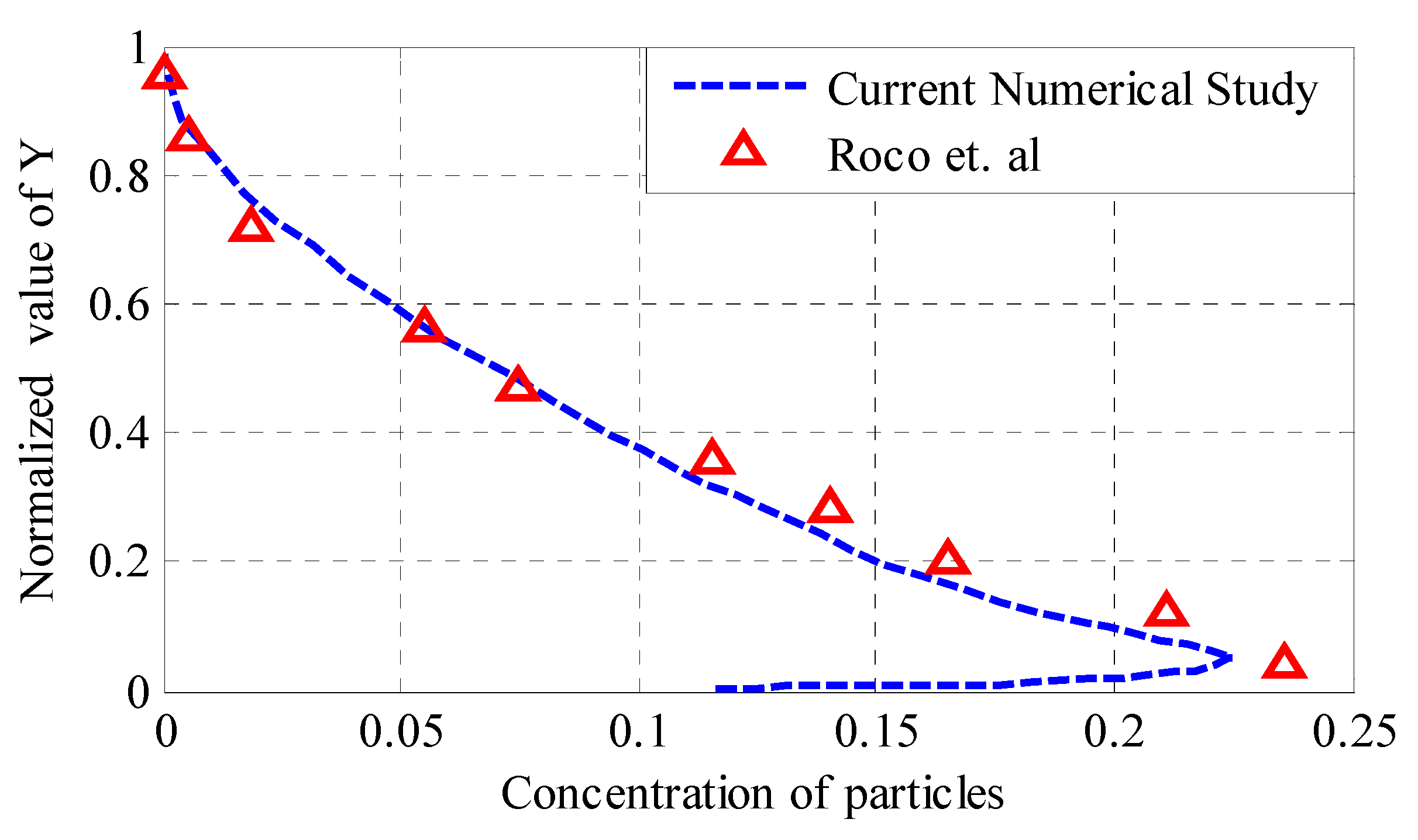
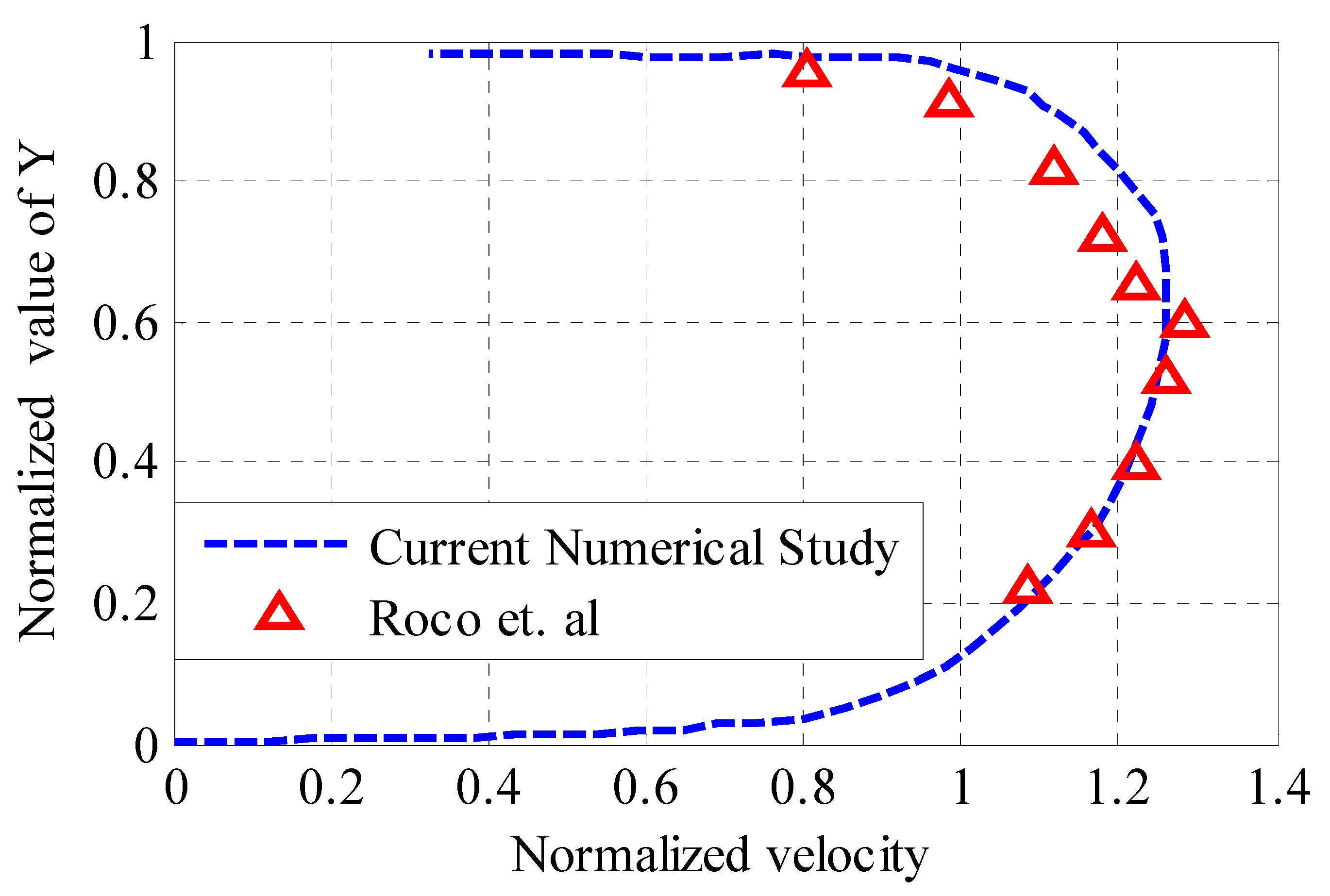
3. Validation of the Numerical Model

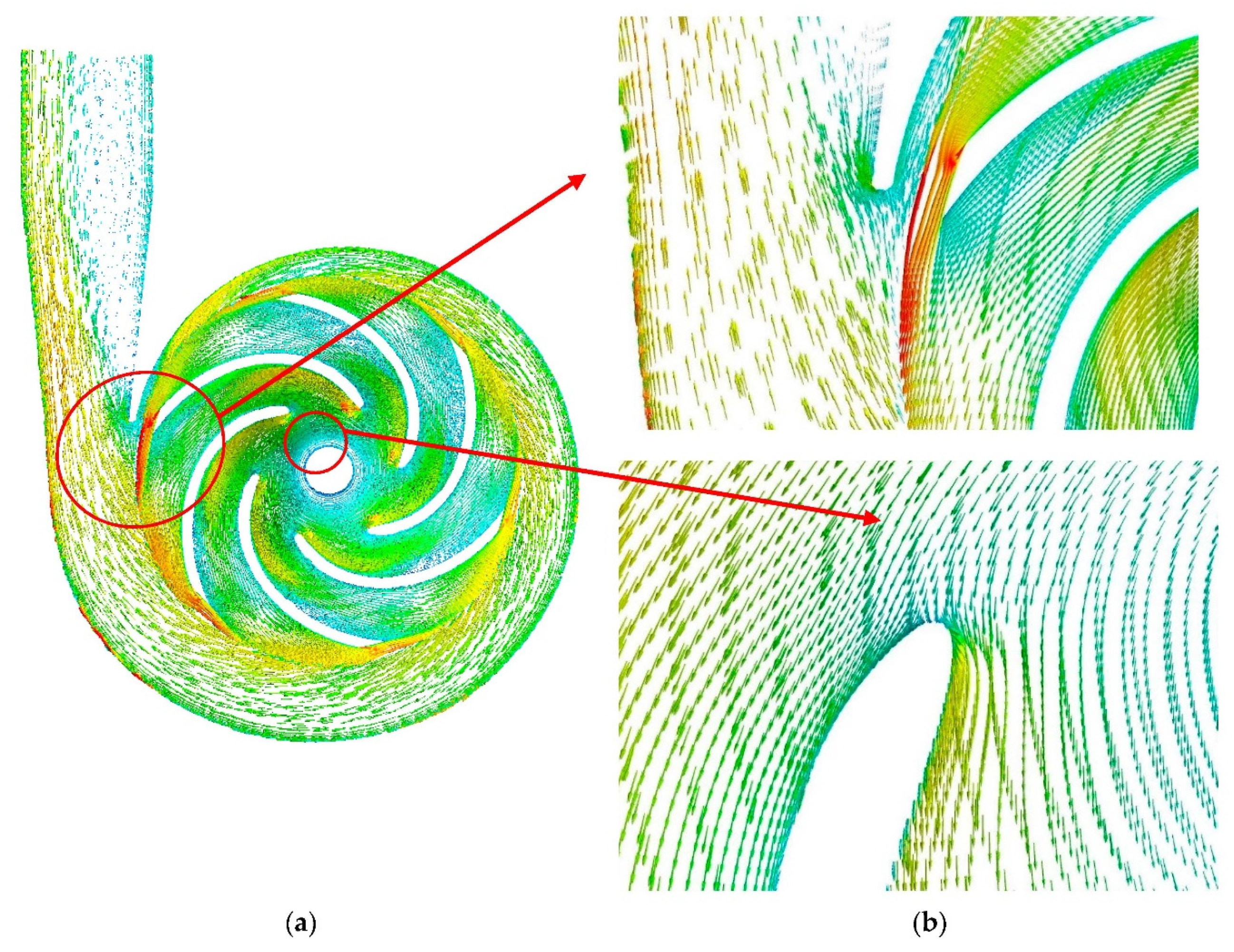
Validation of the current numerical model was carried out by comparing the numerical model employed with the experimental study available in [7]. As there was no data available for the geometry used in the current work, the experimental results accessible in [8] were utilized for validation purposes.

The numerical model present above was employed to compute the erosion rate in the channel used by [8] with dimensions $6 \mathrm{m}\times 2 \mathrm{m}\times 0.05 \mathrm{m}$, as displayed in Figure 3. The diameter of the particles used for the validation work was $165 \mathsf{\mu }\mathrm{m}$ and density was $2680 \mathrm{kg}/{\mathrm{m}}^3$. A uniform volume concentration of the particles, i.e., $8.41\%,$ was imposed at the inlet boundary. While an average velocity at the inlet of the fluid domain was enforced with a value of $1.66 \mathrm{m}/\mathrm{s}$. The same geometry (Figure 3) and other properties mentioned above used by [7] were implemented for the numerical model discussed above. The comparison of the numerical and experimental results is shown in Figure 4 and Figure 5. Figure 4 and Figure 5 show a comparison of experimental results and results produced by the current numerical model comparing particles and velocity profile concentration. The comparison shows that both numerical and reported experimental results [7] were in close agreement, and the present numerical model could predict erosion rate. The same validation procedure has also been adopted in the literature by [14].

4. Results

In the current work, erosion analysis was conducted for the casing and impeller blades of a pump designed and optimized to be used in an industrial application to pump the slurry. The slurry can damage the impeller blades and especially the casing of the pump. Therefore, to estimate and improve the pump’s life, the impact of the particle’s concentration, size, exit flow head, and cavitation was investigated on the erosion rate density of the impeller blades and pump casing.

The qualitative results of the developed pressure and velocity field are displayed in Figure 6 and Figure 7 to support the quantitative results displayed in the following figures. Figure 6a shows the pressure contours on the pump’s casing blades along with the hub, and Figure 6b shows pressure contours on a cut plane passing through 50% span of the blades. It can be observed that pressure in the pump rises in the radial direction (from inlet to outlet). A maximum value of pressure could be observed near the casing walls; then, a dip in pressure was observed near the tongue section of the casing due to a reduction in the cryosection area. This was due to flow acceleration in this region, as can be witnessed in Figure 7a. It can be noted further from Figure 6 and Figure 7, that the pump’s casing acted like a diffuser where the velocity head was converted into the pressure head. The cross-sectional area that was available to the flow was minimum near the tongue section of the casing and increased as the flow moved towards the outlet sections where it was maximum. For the same reason, a maximum value of the local velocity could be observed in the tongue section of the casing. Therefore, the abrupt variation in the cross-sectional area can lead to the complex behavior of the particles in this region that can promote erosion rates in the region.

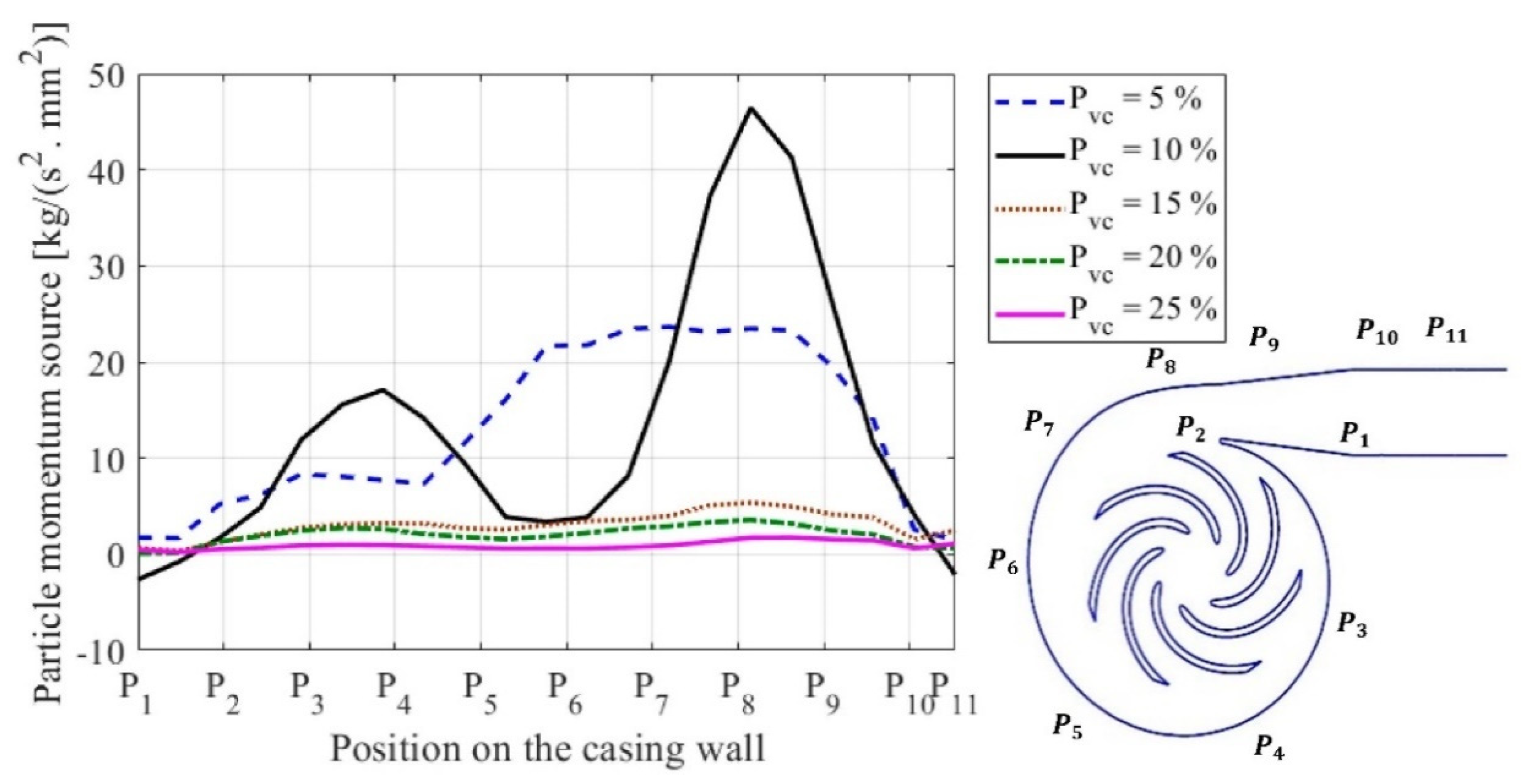
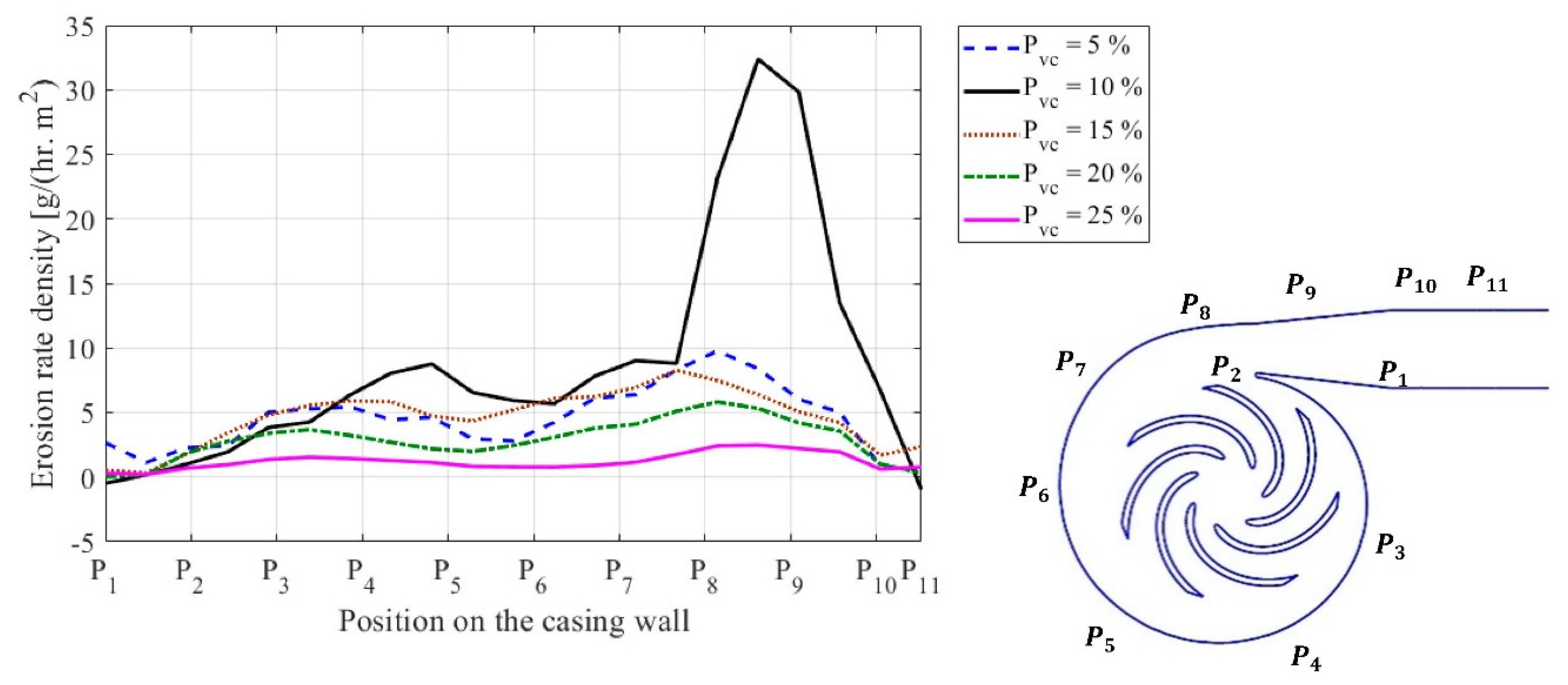
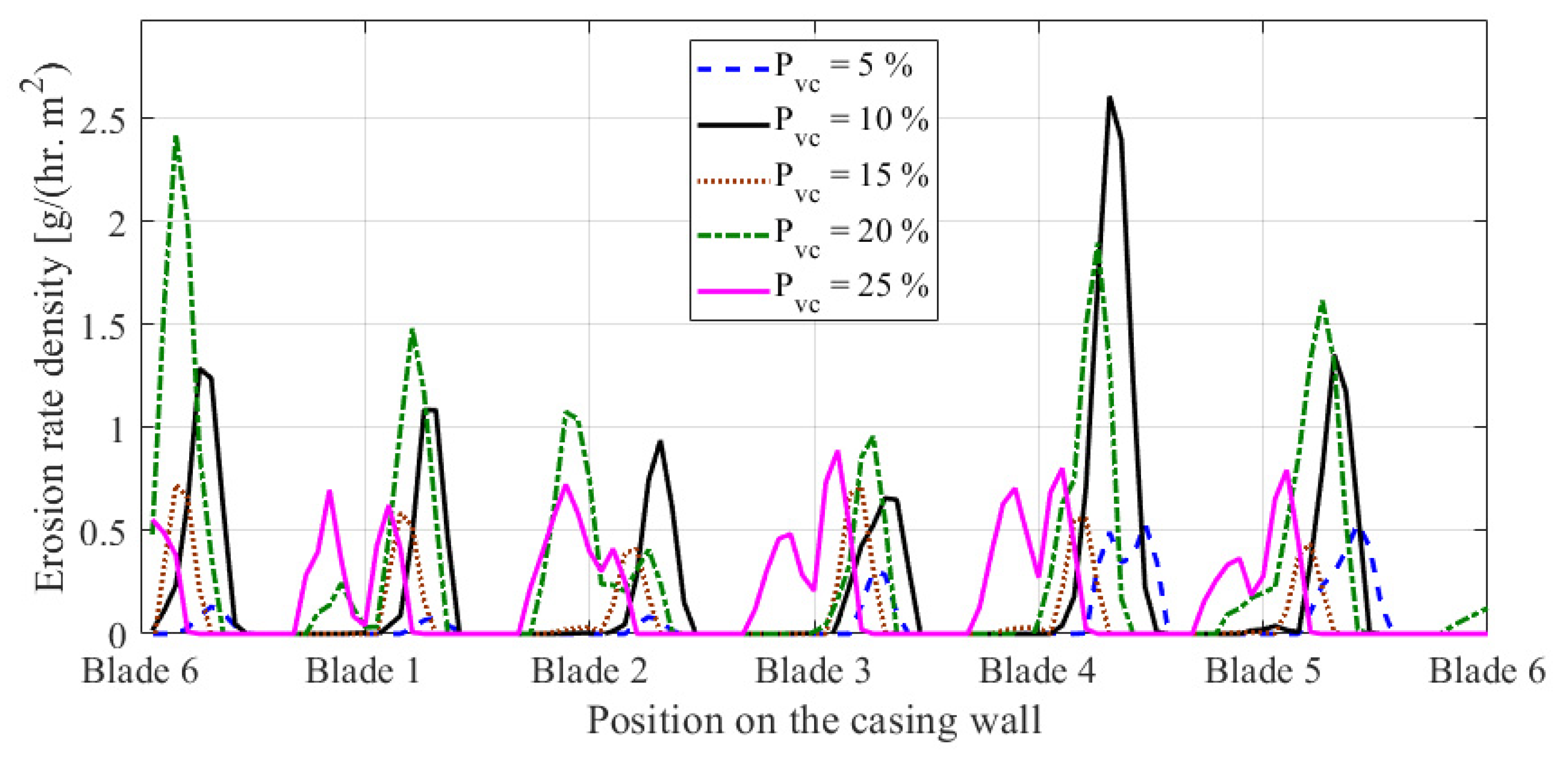
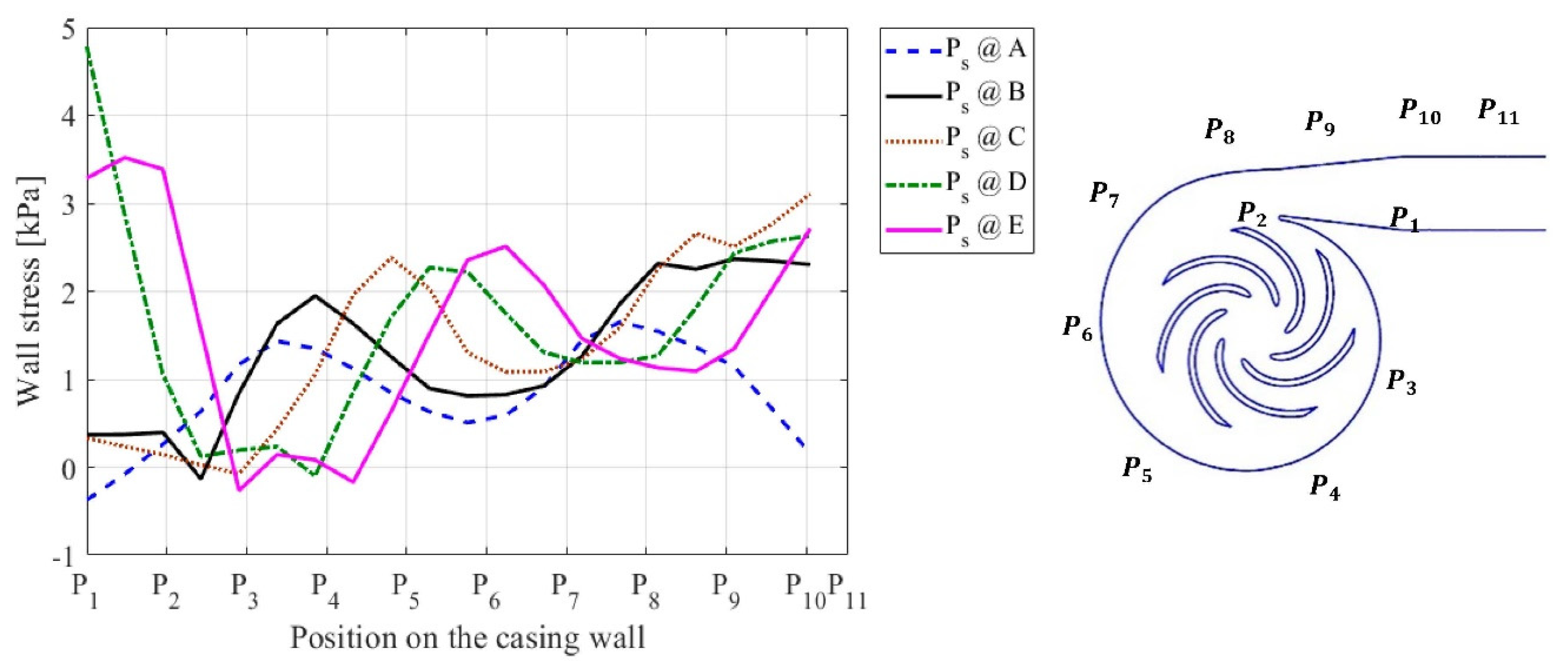
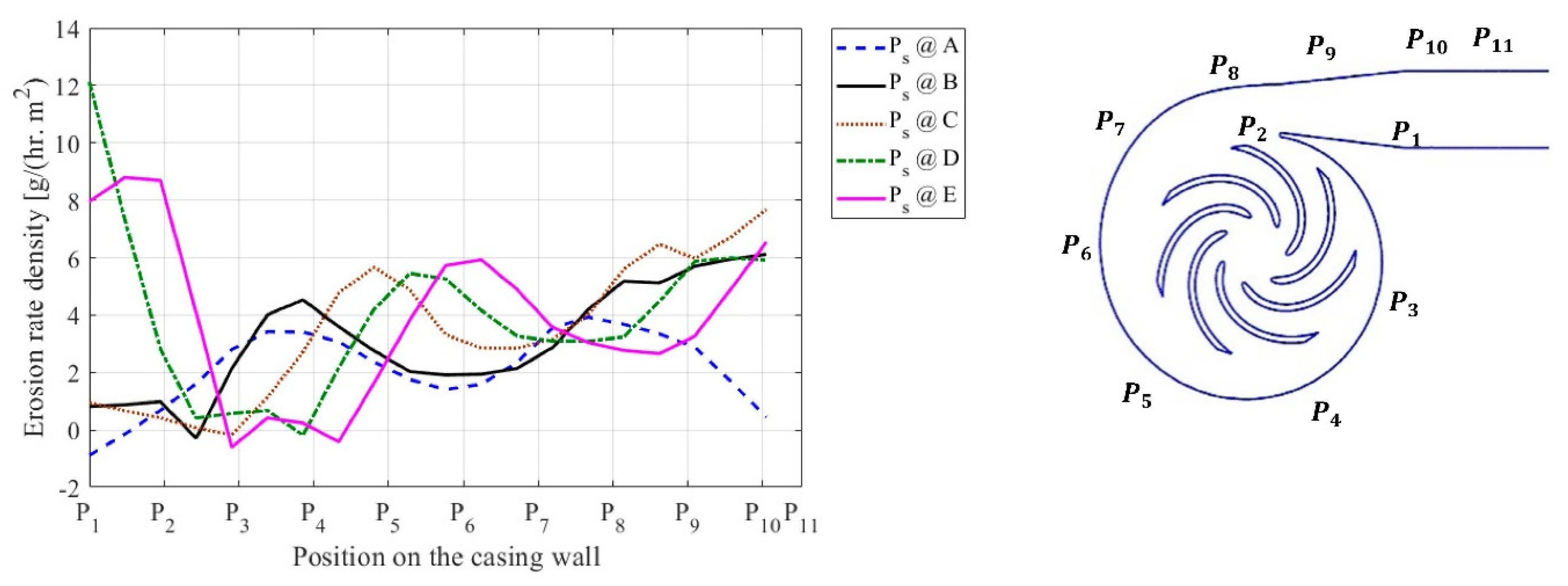
4.1. Effect of the Concentration of Solid Particles

To understand the impact of the concentration of the slurry particles, five different values of particle concentration were studied in the present work, i.e., 5%, 10%, 15%, 20%, and 25%, as indicated in Table 1. Figure 8, Figure 9, Figure 10 and Figure 11 shows particle concentration profiles, wall stress, particle’s momentum source, and erosion rate density along the casing walls from point P1 to P11 for different inlet volumetric concentrations of particles. For all these simulations, particle size distribution A and an exit pressure head of 2.6 bar were employed.

Figure 8 shows that profiles for all particle concentrations, except ${\mathrm{P}}_{\mathrm{vc}}=5\%$, had two peaks of volume concentration. One was near the casing tongue while the second was where the curvature of the casing’s profile suddenly becomes zero. The first peak (around point P₃) was attributed to the smaller cross-section in the region, while the 2nd peak (around point P₈) was due to the sudden change in the casing’s profile. It should be noted that the 2nd peak was much larger than the first. This was because the casing profile changed the direction of the fluid suddenly; however, the particles tended to follow a motion in a straight line as the momentum of the solid particles was higher compared to fluid parties of the same size due to their higher densities. This, in turn, leads to a local cluster of particles in that region after hitting the casing wall.

It is interesting to note here that volume concentration at the casing wall increased initially with the increase in the volume concentration imposed at the inlet boundary (e.g., ${\mathrm{P}}_{\mathrm{vc}}=5 \mathrm{to} 10$); however, with the additional increase in the value of ${\mathrm{P}}_{\mathrm{vc}}$ at the inlet, the concentrations of the particles on the wall started falling. This could be explained based on the fact that with an increase in volume concentration beyond 10%, solid particles from larger chunks, under the action of gravity, started accumulating at the bottom of the casing. As all quantities were measured on the polyline (red polylines in Figure 1) located at the sidewalls, the values of the volumes concentration on the side walls dropped when the inlet value of ${\mathrm{P}}_{\mathrm{vc}} \mathrm{increased}$.

Figure 9 shows wall stress profiles along the casing wall with different volumetric concentrations of the solid particles. A similar trend for the wall stress could be observed for the volume concentration, as discussed above. A maximum value of wall stress was observed for P_vc = 10%, while the minimum values were observed for the full volume concentrations, i.e., P_vc = 25%. The wall stress profiles for P_vc = 5%, 15%, and 20% were identical in terms of values of stress and the location of the two peaks discussed above.

Figure 10 shows the values of the particle momentum source due to the interaction between the two phases. The displayed results suggested that momentum transfer from the water to solid particles changed significantly for the P_vc values of 5% and 10% along the casing wall (P₁ to P₁₁). However, the profiles corresponding to both values of P_vc were quite different from each other. The particle momentum source profile for P_vc = 5% could be characterized by two distinct stable regions, i.e., from P₂ to P₄ and from P₆ to P₉; however, the profile for P_vc = 10% contained two distinctive peaks. The first peak was at P_4, while the second was near P₈. Contrary to the momentum source profiles for P_vc values of 5% and 10%, the profiles corresponding to all other values of P_vc were identical, exhibiting no significant variation along the casing wall.

Figure 11 shows the behavior of erosion rate density along the casing wall with different volumetric concentrations of the solid particles. A significant change in the erosion rate density (ERD) values could be seen along the wall length for P_vc = 10% with two peaks, the first at P₄ while the second was around P₉. Simultaneously, variation in the ERD for all other cases was relatively smaller than the ERD variation along the casing wall at P_vc = 10%. The m aximum value of EDR was found for P_vc = 10%, which was followed by P_vc = 5, P_vc = 15%, and P_vc = 20%. Whereas the minimum value of ERD was observed for P_vc = 25%. It should be noted here that the maximum value of ERD for P_vc = 10% was 10 to 20 times higher than the peak ERD values corresponding to the other cases.

Figure 12 shows the variation of erosion rate density on all six blades in the steam-wise direction (leading to the trailing edge). Displayed data was calculated by extracting the erosion rate density through five polylines at various span locations, i.e., 0%, 25%, 50%, 75%, and 100%. The green-colored polylines, on which data was extracted, can be seen in Figure 1. The Figure suggests that the erosion rate density of the blades was significantly lower than the erosion rate density on the casing walls. Moreover, it could be seen that the maximum value of the ERD was different for different blades depending upon their location.

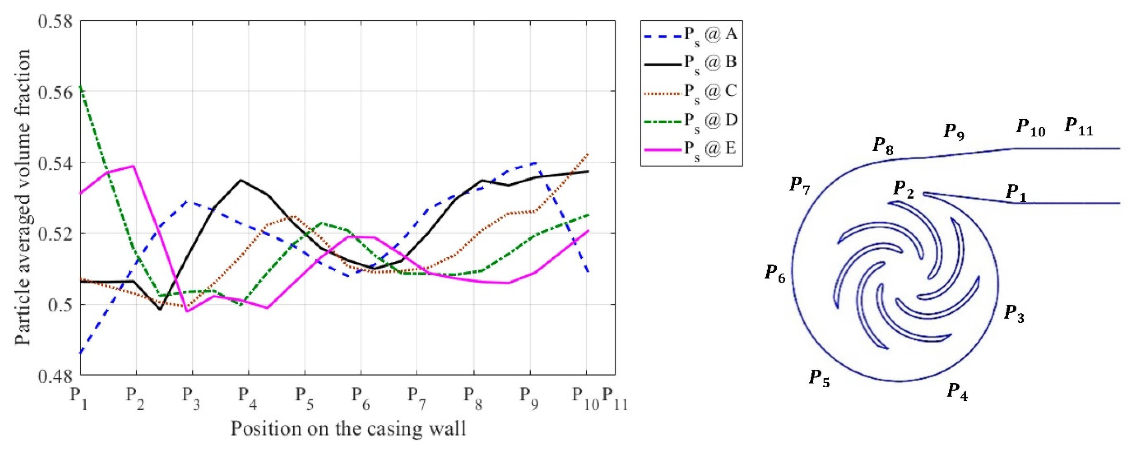
4.2. Effect of Particle Size

In this section, the effects of various particle sizes on the erosion phenomenon in the pump are reported. Five different particle size distributions A, B, C, D, and E, were employed for this study, while the value of the exit pressure (${\mathrm{P}}_{\mathrm{exit}}$) and particle concentrations (P_vc) used were 2.6 bar and 12.5%, respectively. The details on the particle sizes are reported in Table 1.

Figure 13 shows the concentration of the particles on the casing wall at different locations, as indicated on the sketch drawn on the right side of the Figure. Figure 13 shows three peaks of particle averaged volume fraction, i.e., at P, around P_4, and around P₈ which correspond to the exit section, the start of the draft tube section, and just after the casing tongue. This trend holds for all particle sizes except particle size A. For particle size A, the peak mentioned above at P₁ did exist. However, observation of the other two peaks suggested that once the particle size became larger than size A, the physics of the problem changed at the exit section.

A very similar trend for the wall stresses can be seen in Figure 14. Figure 14 suggests that the maximum value of wall stress was found for particle size E (largest among the lot) followed by D and C. The minimum value of the wall stress was found for particle size A. Figure 15 displays a profile of erosion rate density along the casing wall with different solid particle sizes and distribution. Similar to the particle’s concentration profiles indicated above, multiple peaks could be found for the erosion rate density profiles. It should be noted here that the peaks for different particle sizes did not appear at the same locations, but an offset in the peaks could be observed. For example, the peak of the erosion rate density for Ps = A existed just after P_3, while for Ps = B, the peak was delayed and could be seen around P₄.

The peak for the maximum particle size (Ps= B) was delayed the most and could be observed at P₆. Furthermore, the value of the ERD increased slightly with the increase in particle size. The maximum value of the erosion rate density (ERD) could be found for Ps = E, followed by Ps = D and Ps = C, while the minimum value of the erosion rate density was observed for Ps = A.

Figure 16 shows the variation of erosion rate density on all six blades in the steam-wise direction. (leading to the trailing edge) with different values of solid particle size and distribution. The Figure suggests that the erosion rate density of the blades was significantly lower than the erosion rate density on the casing walls. It could also be noted that the maximum value of the ERD was different at different blades depending upon their location. The maximum value of the erosion rate density could be observed near the leading edges for all blades. In contrast, erosion rate densities corresponding to the region between the leading and trailing edges were minimal.

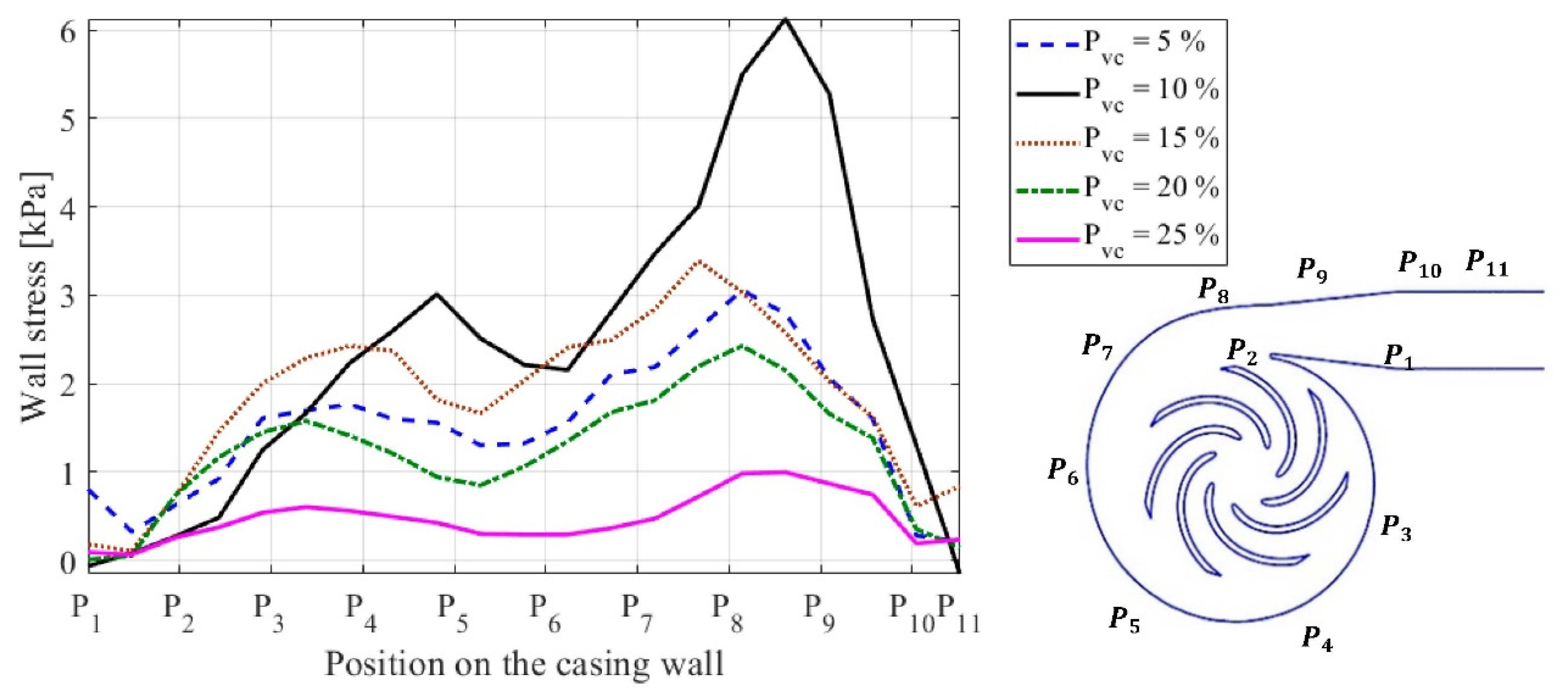
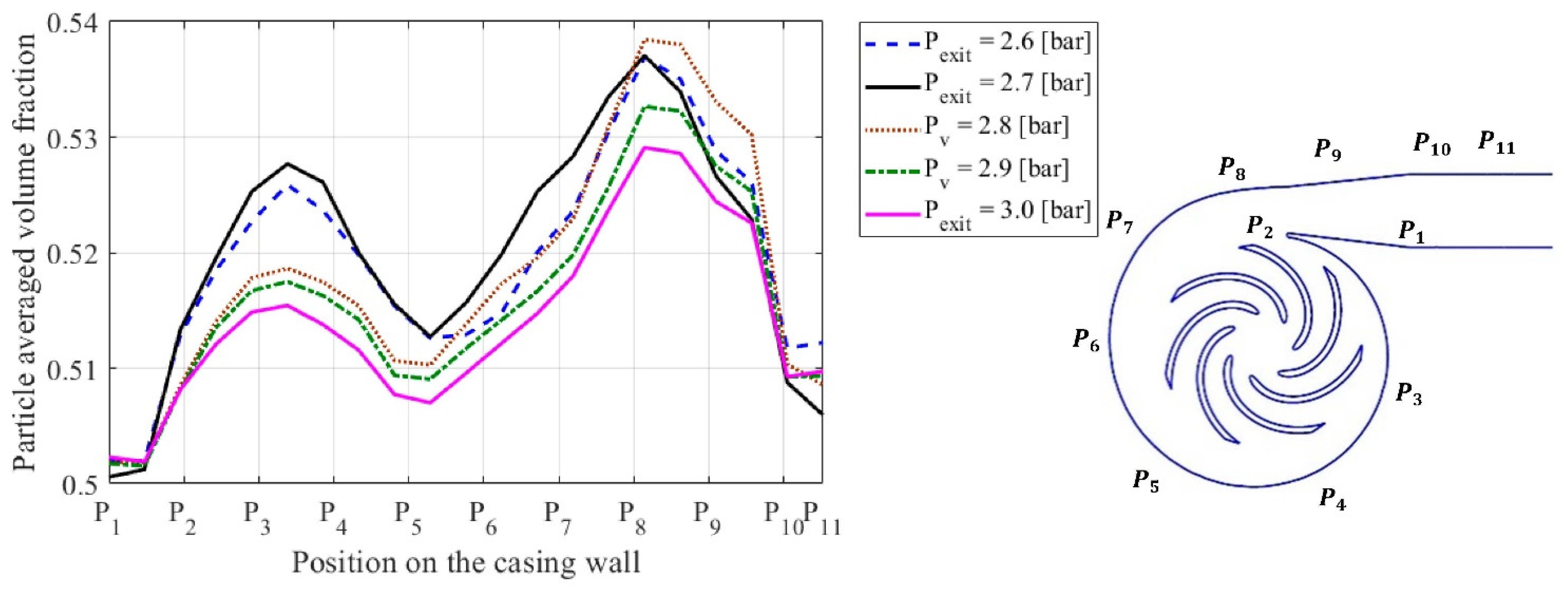
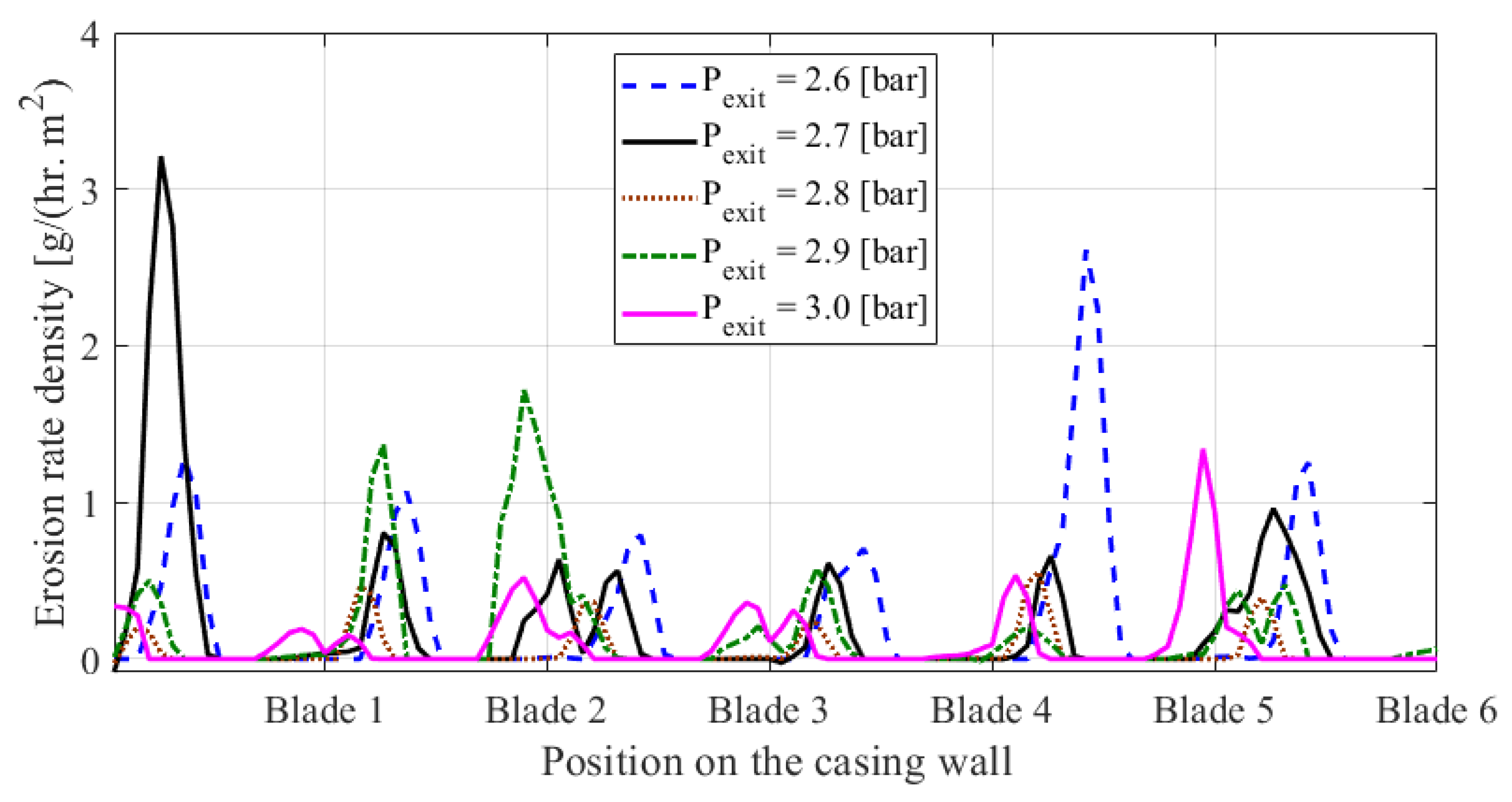
4.3. Effect of the Exit Pressure Head Conditions on Erosion Rates

Five conditions were investigated in the current study to understand the effect of the pump’s exit pressure head-on erosion characteristics. Exit pressure conditions employed for the present work were 2.6 bar, 2.7 bar, 2.8 bar, 2.9 bar, and 3.0 bar. At the same time, the value of the particle’s size and particle volume concentration used for the current study were P_A and 12.5%, respectively.

Figure 17, Figure 18 and Figure 19 show the particle’s concentration, particle’s momentum source, wall stress, and erosion rate density profiles along the casing wall (P₁–P₁₁). The overall behavior of the profiles for the parameters mentioned above was almost identical. Profiles from all parameters exhibited two peaks, the first peak existed just after the tongue of the casing, and the second just at the start of the draft pipe section of the casing. The second peak was relatively higher than the first for all the parameters mentioned above.

Figure 17 shows the variation of concentration of particles along the casing wall with different values of exit pressure heads. The value of the particle’s concentration increased initially with the increase in the value of the exit pressure from 2.6 bar to 2.7 bar and then decreased when the exit pressure increased from 2.7 bar to 3.0 bar. Figure 18 shows trends of the particle’s momentum source along the casing wall with different values of exit pressure heads. The maximum and minimum values of the momentum transfer from water to particle were found for P_exit = 2.6 and 3.0, respectively. On the contrary, the erosion rate density increased with an increase in the value of exit pressure, as shown in Figure 19. The maximum and minimum values of the erosion rate density increased corresponding to P_exit = 3.0 and 2.6, respectively.

It should be noted here that ERT increased substantially when the exit pressure increased from 2.6 bar to 2.8 bar, while on a further increase from 2.8 bar to 3.0 bar, the rise in the value of erosion rate density was very small. Figure 20 shows the variation of erosion rate density on all six blades in the steam-wise direction (leading to trailing edge) corresponding to various values of the exit pressure. The Figure 20 suggests that the erosion rate density of the blades was significantly lower than the erosion rate density on the casing walls, as was the case with particle size and particle concentration. Additionally, it could be seen that the maximum value of the ERD was different at the different blades depending upon their location.

4.4. Effect of Cavitation

To study the impact of the cavitation on the erosion characteristics, the conditions (pressure in the blade passage should drop below the saturation pressure of the water) under which cavitation may occur were found. It was noticed that cavitation might be introduced in the blade passage at a higher flow rate, i.e., $\frac{Q_{\eta }}{Q_{\eta \left(max\right)}}=2.7$. Here, Q_η is the minimum required value of flow rate to trigger the cavitation, while Q_η(max) is the flow rate that corresponds to the maximum efficiency of the pump. A higher flow rate resulted in greater velocity values in the blade passage. The pressure became lower than the saturation pressure of the liquid in the region around the entry section of the blades. Contours of the water vapor volume fraction and mass fraction are displayed in Figure 21a. A sturdy bubble pattern could be noticed on the blade’s suction side triggered from the blade’s leading edge. Some shaky bubble fields could also be observed on the pressure side near the blade’s trailing edge. Velocity vectors in the blade channels with no cavitation and with cavitation are shown in Figure 21b,c. Figure 21b indicates that the velocity vectors were aligned with the blade passage, and no recirculation region could be observed for the case with no cavitation. At the same time, in Figure 21c, a huge recirculation region can be spotted in the suction which was triggered by the bubble structure initiating from the leading edge of the blade. There was also a minor separation region on the pressure side of the blade that was an outcome of small-scale cavitation taking place on the pressure side. Owing to these dead zones in the passage developed by the bubble structures, the development of local velocities in the passage and at the trailing edge grew substantially.

Figure 22 shows the erosion rate density distribution for different concentrations of particles under the cavitation conditions. Comparison of the results in Figure 11 and Figure 22 indicated that cavitation shifts the location of the peaks towards the exit of the pump, and the magnitude of the location of the erosion rate intensity increased noticeably.

5. Conclusions

The current study is performed on an optimized pump geometry to forecast the impact of solid particle concentration, size, distribution, exit pressure heads, and cavitation on the erosion rate density of the pump casing. The following deductions have been made from the above-given results.

The concentration of the solid particles substantially affects the magnitude of erosion characteristics of the pump casing and impeller blade, followed by the pump’s exit pressure heat. On the contrary, the particle size and cavitation do not alter the erosion rates significantly but appreciably influence the regions of high erosion rate densities. The inlet concentration of the solid particles significantly impacts the erosion rate density, and it changes from 5% to 20% and doubles the erosion rate density at particular points.

The maximum values for the erosions rates are found around the tongue region of the casing and in the vicinity of the exit section of the volute casing. It is found that variation in the erosion rate density, particle concentration, and wall stress changes substantially along with the pump casing (P₁ to P₁₁) and its sensitivity at lower concentrations of the particles. The maximum value of the erosion rate density is found at 10% concentration, and a further increase in the particle concentration will decrease the erosion rate density.

Particle size has no substantial effect on the magnitude of the erosion rate density; however, the location of the ERD peak changes with a change in the size of the particles.

The value of the erosion rate density changes substantially (up to five times) by changing the exit pressure. The maximum values of the erosion rate density were found at the design value pressure head. The value of the erosion rate density decreases by decreasing the exit pressure head value.

Results suggest that the blades’ erosion density is significantly lower than the erosion rate density on the casing walls in all cases. The maximum value of the ERD is different for different blades depending upon their location. The maximum value of the erosion rate density can be observed near the leading edges for all blades. In contrast, erosion rate densities corresponding to the region between the leading and trailing edges are minimal.

References

1. Wilson, K.C. Principles of Particulate Slurry Flow. In Slurry Transport Using Centrifugal Pumps, 3rd ed.; Springer: New York, NY, USA, 2006; pp. 83–101. [Google Scholar]
2. Wilson, K.C. Centrifugal Pumps. In Slurry Transport Using Centrifugal Pumps, 3rd ed.; Springer: New York, NY, USA, 2006; pp. 190–226. [Google Scholar]
3. Wilson, G. The Effects of Slurries on Centrifugal Pump Performance. In Fourth International Pump User Symposium; 1987; pp. 19–26. Available online: http://turbolab.tamu.edu/proc/pumpproc/P4/P419-25.pdf (accessed on 15 February 2021).
4. Roco, M.C.; Cader, T. Numerical Method to Predict Wear Distribution in Slurry Pipelines. In Advances in Pipe; Protection, G., Thorns, J.J., Eds.; BHRA Fluid Engineering: Cranfield, UK, 1988; pp. 53–85. [Google Scholar]
5. Roco, J.; Nair, M.C.; Addie, P.; Dennis, G.R. Erosion of concentrated slurry in turbulent flow. ASME FED 1984, 13, 69–77. [Google Scholar]
6. Minemura, T.; Uchiyama, K. Calculation of the Three-Dimensional Behavior of Spherical Solid Particles Entrained in a Radial-Flow Impeller Pump. Proc. Int. Mech. Eng. 1990, 204, 159–166. [Google Scholar]
7. Roco, C.; Addie, G.R. Analytical Model and Experimental studies on Slurry flow and erosion in pump casings. Slurry Transp. 1983, 8, 263–275. [Google Scholar]
8. Roco, R.J.; Addie, M.C.; Visintainer, G.R. Study of Casing Performances in Centrifugal Slurry Pumps. Part. Sci. Technol. 1985, 3, 65–88. [Google Scholar] [CrossRef]
9. Pagalthivarthi, K.V.; Ravi, M.R.; Gupta, P.K.; Tyagi, V. CFD Prediction of Erosion Wear in Centrifugal Slurry Pumps for Dilute Slurry Flows. J. Comput. Multiph. Flows 2011, 3, 225–245. [Google Scholar] [CrossRef] [Green Version]
10. Zhong, Y.; Minemura, K. Measurement of erosion due to particle impingement and numerical prediction of wear in pump casing. Wear 1996, 199, 36–44. [Google Scholar] [CrossRef]
11. Addie, J.R.; Pagalthivarthi, G.R.; Kadambi, K.V. PIV and Finite Element Comparisons of Particles Inside a Slurry Pump Casing. In Proceedings of the International Conference on Hydrotransport 16, Santiago, Chile, 26–28 April 2004; pp. 547–559. [Google Scholar]
12. Charoenngam, G.R.; Subramanian, P.; Kadambi, A.; Addie, J.R. Investigations of Slurry Flow in a Centrifugal Pump Using Particle Image Velocimetry. In Proceedings of the 4th International conference on multiphase flow, New Orleans, LA, USA, 27 May–1 June 2001. [Google Scholar]
13. Versteeg, H.K.; Malalasekera, W. An Introduction to Computational Fluid Dynamics: The Finite Volume Method; Pearson Education: London, UK, 2007. [Google Scholar]
14. Pagalthivarthi, K.V.; Gupta, P.K.; Tyagi, V.; Ravi, M.R. CFD Predictions of Dense Slurry Flow in Centrifugal Pump Casings. World Acad. Sci. Eng. Technol. Int. J. Mech. Aerospace, Ind. Mechatron. Manuf. Eng. 2011, 5, 538–550. Available online: https://www.waset.org/Publications/cfd-predictions-of-dense-slurry-flow-in-centrifugal-pump-casings/3699?p=2 (accessed on 14 March 2017).
15. Brown, G. Use of CFD to Predict and Reduce Erosion in an Industrial Slurry Piping System. Available online: http://www.cfd.com.au/cfd_conf06/PDFs/073Bro.pdf (accessed on 11 March 2017).
16. Saeed, M.; Berrouk, A.S.; Siddiqui, M.S.; Awais, A.A. Effect of printed circuit heat exchanger’s different designs on the performance of supercritical carbon dioxide Brayton cycle. Appl. Therm. Eng. 2020, 179, 115758. [Google Scholar] [CrossRef]
17. Saeed, M.; Alawadi, K.; Kim, S.C. Performance of Supercritical CO2 Power Cycle and Its Turbomachinery with the Printed Circuit Heat Exchanger with Straight and Zigzag Channels. Energies 2020, 14, 62. [Google Scholar] [CrossRef]
18. Salim, M.S.; Saeed, M.; Kim, M.-H. Performance Analysis of the Supercritical Carbon Dioxide Re-compression Brayton Cycle. Appl. Sci. 2020, 10, 1129. [Google Scholar] [CrossRef] [Green Version]
19. Menter, F.R.; Eloret, S. Zonal two equation kappa-omega turbulence models for aerodynamic flows. In Proceedings of the 23rd Fluid Dynamics, Plasmadynamics, and Lasers Conference, Orlando, FL, USA, 6–9 July 1993. [Google Scholar]
20. Siddiqui, M.S.; Latif, S.T.M.; Saeed, M.; Rahman, M.; Badar, A.W.; Hasan, S.M. Reduced order model of offshore wind turbine wake by proper orthogonal decomposition. Int. J. Heat Fluid Flow 2020, 82, 108554. [Google Scholar] [CrossRef]
21. Saeed, M.; Berrouk, A.S.; Siddiqui, M.S.; Awais, A.A. Numerical investigation of thermal and hydraulic characteristics of sCO2-water printed circuit heat exchangers with zigzag channels. Energy Convers. Manag. 2020, 224, 113375. [Google Scholar] [CrossRef]
22. Ha, S.T.; Ngo, L.C.; Saeed, M.; Jeon, B.J.; Choi, H. A comparative study between partitioned and monolithic methods for the problems with 3D fluid-structure interaction of blood vessels. J. Mech. Sci. Technol. 2017, 31, 281–287. [Google Scholar] [CrossRef]
23. Saeed, M.; Awais, A.A.; Berrouk, A.S. CFD aided design and analysis of a precooler with zigzag channels for supercritical CO2 power cycle. Energy Convers. Manag. 2021, 236, 114029. [Google Scholar] [CrossRef]
24. Saeed, M.; Berrouk, A.S.; AlShehhi, M.S.; AlWahedi, Y.F. Numerical investigation of the thermohydraulic characteristics of microchannel heat sinks using supercritical CO2 as a coolant. J. Supercrit. Fluids 2021, 176, 105306. [Google Scholar] [CrossRef]
25. Awais, A.A.; Saeed, M.; Kim, M.-H. Performance enhancement in minichannel heat sinks using supercritical carbon dioxide (sCO2) as a coolant. Int. J. Heat Mass Transf. 2021, 177, 121539. [Google Scholar] [CrossRef]
26. Cai, X.; Gu, R.; Pan, P.; Zhu, J. Unsteady aerodynamics simulation of a full-scale horizontal axis wind turbine using CFD methodology. Energy Convers. Manag. 2016, 112, 146–156. [Google Scholar] [CrossRef]
27. Sayed, M.A.; Kandil, H.; Shaltot, A. Aerodynamic analysis of different wind-turbine-blade profiles using finite-volume method. Energy Convers. Manag. 2012, 64, 541–550. [Google Scholar] [CrossRef]
28. Sørensen, N.N.; Michelsen, J.A.; Schreck, S. Navier-Stokes predictions of the NREL phase VI rotor in the NASA Ames 80 ft × 120 ft wind tunnel. Wind. Energy 2002, 5, 151–169. [Google Scholar] [CrossRef]
29. Saeed, M.; Kim, M.-H. Thermal and hydraulic performance of SCO2 PCHE with different fin configurations. Appl. Therm. Eng. 2017, 127, 975–985. [Google Scholar] [CrossRef]
30. Saeed, M.; Kim, M.-H. Airborne wind turbine shell behavior prediction under various wind conditions using strongly coupled fluid structure interaction formulation. Energy Convers. Manag. 2016, 120, 217–228. [Google Scholar] [CrossRef]
31. Saeed, M.; Kim, M.-H. Aerodynamic performance analysis of an airborne wind turbine system with NREL Phase IV rotor. Energy Convers. Manag. 2017, 134, 278–289. [Google Scholar] [CrossRef]
32. Van Bussel, G.J.W. The science of making more torque from wind: Diffuser experiments and theory revisited. J. Phys. Conf. Ser. 2007, 75, 012010. [Google Scholar] [CrossRef]
33. Hansen, M.O.L.; Sørensen, N.N.; Flay, R.G.J. Effect of Placing a Diffuser around a Wind Turbine. Wind. Energy 2000, 3, 207–213. [Google Scholar] [CrossRef]
34. Hutchings, I. Mechanical and metallurgical aspects of the erosion of metals. In Proceedings of the International Conference on Corrosion-Erosion of Coal Conversion System Materials, Berkeley, CA, USA, 24–26 January 1979; pp. 393–427. [Google Scholar]
35. Finnie, I. Some observations on the erosion of ductile metals. Wear 1972, 19, 81–90. [Google Scholar] [CrossRef]
36. Franc, J.P. The Rayleigh-Plesset equation: A simple and powerful tool to understand various aspects of cavitation. In Fluid Dynamics of Cavitation and Cavitating Turbopumps; Springer: Berlin/Heidelberg, Germany, 2007; pp. 1–41. [Google Scholar]
37. ANSYS CFX. CFX-Pre User’s Guide Release 16.0; Ansys Inc.: Canonsburg, PA, USA, 2015. [Google Scholar]
38. Siddiqui, M.S.; Khalid, M.H.; Zahoor, R.; Butt, F.S.; Saeed, M.; Badar, A.W. A numerical investigation to analyze effect of turbulence and ground clearance on the performance of a roof top vertical-axis wind turbine. Renew. Energy 2021, 164, 978–989. [Google Scholar] [CrossRef]
Figure 1. Computational domain and boundary conditions and polylines used for the data postprocessing.
Applsci 11 07364 g001
Figure 2. Mesh for rotating and stationary domains.
Applsci 11 07364 g002
Figure 3. (a) geometrical model and boundary locations (b) mesh of the computational model.
Applsci 11 07364 g003aApplsci 11 07364 g003b
Figure 4. Comparison of numerical and experimental results for the concentration of particles.
Applsci 11 07364 g004
Figure 5. Comparison of experimental and numerical results of the velocity profile.
Applsci 11 07364 g005
Figure 6. (a) Pressure contours on the pump casing, Blades, and hub, (b) Pressure contours on a cut plane passing through a 50% span of the blades while the volume concentration of the particles is 5%, (c) legend.
Applsci 11 07364 g006
Figure 7. Velocity vectors on a cut plane passing through a 50% span of the blades (b) exaggerated views at the leading and trailing edges of the blade at a 50% span.
Applsci 11 07364 g007
Figure 8. Variation of the concentration of particles along the casing wall with different values of volumetric concentration of the solid particles.
Applsci 11 07364 g008
Figure 9. Wall stress profiles along the casing wall with different values of volumetric concentration of the solid particles.
Applsci 11 07364 g009
Figure 10. Variation of particles momentum source along the casing wall with different values volumetric concentration of the solid particles.
Applsci 11 07364 g010
Figure 11. Variation of erosion rate density along the casing wall with different values volumetric concentration of the solid particles.
Applsci 11 07364 g011
Figure 12. Variation of erosion density rate on the blade walls with different values volumetric concentration of the solid particles.
Applsci 11 07364 g012
Figure 13. Variation of the concentration of particles along the casing wall with different solid particle sizes and distribution.
Applsci 11 07364 g013
Figure 14. Variation of concentration of wall stresses along the casing wall with different solid particle sizes and distribution.
Applsci 11 07364 g014
Figure 15. Variation of erosion rate density along the casing wall with different solid particle sizes and distribution.
Applsci 11 07364 g015
Figure 16. Variation of erosion density rate on the blade walls with different solid particles size and distribution values.
Applsci 11 07364 g016
Figure 17. Variation of concentration of particles along the casing wall with different values of exit pressure heads.
Applsci 11 07364 g017
Figure 18. Trends of the particle’s momentum source along the casing wall with different values of exit pressure heads.
Applsci 11 07364 g018
Figure 19. Variation of concentration of particles along the casing wall with different values of exit pressure heads.
Applsci 11 07364 g019
Figure 20. Variation of concentration of particles along the casing wall with different values of exit pressure heads.
Applsci 11 07364 g020
Figure 21. (a) Volume concentration of water vapor contours in the blade passage (b) Velocity vectors in the blade channels with no cavitation, (c) Velocity vectors in the blade channels with cavitation while volume concentration of the particles is 5%.
Applsci 11 07364 g021
Figure 22. Erosion density rate distribution for different concentrations of particles under the cavitation conditions.
Applsci 11 07364 g022