Article

A Novel Acceleration-Based Moving Force Identification Algorithm to Detect Global Bridge Damage

School of Civil Engineering, University College Dublin, Belfield, D04 V1W8 Dublin, Ireland
*
Author to whom correspondence should be addressed.
Appl. Sci. 2021, 11(16), 7271; https://doi.org/10.3390/app11167271
Submission received: 5 July 2021 / Revised: 30 July 2021 / Accepted: 4 August 2021 / Published: 7 August 2021
(This article belongs to the Special Issue State-of-the-Art Structural Health Monitoring in Civil Engineering)

Abstract

:

Featured Application

Acceleration based moving force identification is applied for weigh in motion and bridge damage detection purposes.

Abstract

This paper presents a new moving force identification (MFI) algorithm that uses measured accelerations to infer applied vehicle forces on bridges. Previous MFI algorithms use strain or deflection measurements. Statistics of the inferred forces are used in turn as indicators of global bridge damage. The new acceleration-based MFI algorithm (A-MFI) is validated through numerical simulations with a coupled vehicle-bridge dynamic interaction model programmed in MATLAB. A focussed sensitivity study suggests that results are sensitive to the accuracy of the vehicle velocity data. The inferred Gross Vehicle Weight (GVW), calculated by A-MFI, is proposed as the bridge damage indicator. A real weigh-in-motion database is used with a simulation of vehicle/bridge interaction, to validate the concept. Results show that the standard deviation of inferred GVWs has a good correlation with the global bridge damage level.

1. Introduction

Bridges are critical components in traffic networks but may be damaged by corrosion or may be struck by a vehicle passing underneath. Monitoring of the structural health of bridges is integral to most transport infrastructure management programmes. While most bridges are still monitored by subjective visual inspection, electronic structural health monitoring (SHM) has attracted increasing attention in recent years. Farrar et al. [1] summarise a typical SHM process as (a) the definition of damage: local or global; (b) data acquisition, fusion, and cleaning: what kind of data is used and how; (c) feature extraction: what information is extracted from the data; and (d) statistical model development: how to model structural damage with the extracted information. The method presented in this paper infers gross vehicle weight (GVW) data from bridge acceleration signals and uses the standard deviation of the inferred GVW data to detect bridge global damage. Generally, structural damage refers to changes in the system which result in current or future adverse impacts on its performance [2]. Some data can show damage directly, such as crack width, but this requires advanced knowledge of where the damage is located. Other data, such as strains, deflections, rotations, and accelerations, can also be used as indirect damage indicators. Carden and Fanning [3] identify several features that can be extracted from bridge vibration information, such as natural frequency, mode shape, modal curvature, dynamically measured flexibility, and more. Most researchers use accelerations to find bridge mode shapes and natural frequencies, which are used as indicators of damage in SHM [3,4,5]. However, the natural frequency is insensitive to damage, and mode shape generally requires large numbers of sensors.
By using bridge vibration information, not only bridge properties but also passing vehicle weights can be extracted. Cantero and González [6] showed that if there is an overall reduction in the bridge stiffness, the inferred vehicle weights increase, i.e., the more flexible bridge infers GVWs that are greater than the actual weights. The weights of passing vehicles can be obtained from recorded bridge monitoring data in a process known as Bridge Weigh in Motion (BWIM). The BWIM concept was introduced in the 1970s by Moses [7] who proposed an algorithm to calculate weights from strain measurements on the bridge. Lydon et al. [8] summarise methods that use bridge measurements to find passing vehicle weights. Most BWIM methods use bridge strain or deflections. In practice, most deflection measurement methods require a reference point to measure from, normally under the bridge, which can be problematic as such a point is not always available (e.g., when the bridge is over water). Recently, a contactless BWIM system was proposed that used image analysis technology to measure bridge deflections and infer GVWs from them [9,10]. The drawback of contactless BWIM is that the accuracy depends on the performance of the image collection equipment which is not generally sufficiently accurate. Also, it requires a known weight truck for setup or to recalibrate. Compared with deflection, acceleration measurement is inertial, so it does not require a reference point. Recently, some researchers have tried to use bridge acceleration to find passing vehicle weights. Mohammed and Uddin [11] proposed an approach to use bridge acceleration to estimate bridge displacement by using a state vector estimation. The moving force identification (MFI) algorithm is then used to estimate vehicle weights. Sekiya et al. [12] used an acceleration-based free vibration method to determine bridge displacement and then used the bridge influence line to calculate passing vehicle weights. The main problem with the approach, which uses acceleration to get bridge displacement, relates to knowing the bridge’s initial conditions. As described by Park et al. [13] inadequate bridge initial conditions can cause large errors in estimated displacements. Researchers have adopted different approaches to reduce this error [14,15]. To the author’s knowledge, only two researchers have used accelerations directly in BWIM or MFI systems [16,17]. Law et al. [16] proposed an MFI algorithm in the time domain, which can use acceleration signals directly. However, the force response cannot be obtained from the acceleration data alone—bending moment data is also required. OBrien et al. [17] introduced the concept of an acceleration-based influence line and applied it to BWIM. The issue with this method is that the magnitude of vehicle acceleration can be strongly affected by the road profile, which affects the accuracy. While the accuracy of this acceleration-based BWIM method is low, the authors demonstrated that the inferred vehicle weights obtained from a large sample of passing trucks can be used to infer damage. A different approach is taken in this paper, where acceleration is used to extract vehicle axle force, which is not strongly affected by the profile.
To find a method that can directly use acceleration and estimate GVW with good accuracy, an MFI algorithm is chosen. MFI has been proposed as a method of BWIM that potentially can give more accurate and more detailed results than the traditional approach [18,19,20]. Several forms of the MFI algorithm exist but all derive axle force histories from the equations of motion [21,22,23,24,25]. A popular approach, which is introduced by Trujillo [26], uses the state-space form of the dynamic equations to solve this inverse problem. In the state space approach, the 2nd order differential equation governing displacement is replaced by two 1st order equations that are solved simultaneously to find the displacements and velocities [27]. Numerical instability is a challenge, with many examples giving ill-conditioned solutions [28]. Zhu et al. [28] apply Tikhonov regularization [29] to improve the conditioning of the system of equations, which significantly improves the accuracy. Gonzalez et al. [18] further develop this algorithm by regularizing the first derivative of force to make the solution smoother and more stable. Rowley et al. [30] validate the algorithm of Gonzalez et al. [18] using strain data measured on a bridge in service and achieve good accuracy. The majority of BWIM and MFI approaches use strain and a few use deflection or rotation, but acceleration has only recently been considered [17]. Few researchers have used vehicle axle force, computed by MFI from bridge deflection data, to detect damage [31,32,33]. They show that the bridge’s local damage will significantly affect inferred force results. As the bridge becomes damaged, bridge deflections will increase and the inferred force will be overpredicted. This principle cannot be applied when acceleration is used as acceleration magnitude is affected by the road profile.
In this paper, the new acceleration-based MFI (A-MFI) algorithm is applied directly to acceleration data, requiring reformulation of the underlying equations. Unlike strain data, used in previous studies, acceleration data is damage sensitive, suggesting that it has good potential to be used as part of a bridge health monitoring approach. The concept is assessed using a numerical simulation with a half-car vehicle/bridge interaction model and a finite element model of a bridge. A sensitivity study is carried out on potential sources of error such as the scan rate of measurements, imperfect velocity measurement, pre-existing vibrations, and measurement noise. The study demonstrates that acceleration-based MFI-inferred vehicle weight data is a good indicator of bridge global damage. Global damage is considered in this study, i.e., an overall loss of stiffness. This type of damage may be due to multiple small local damages or to uniform corrosion damage over time.

2. Acceleration Based Moving Force Identification Theory

Most MFI approaches have been derived from a solution to the equations of motion of a bridge. The equations of motion representing the dynamic response can be expressed as:
[ M g ] { u ¨ } + [ C g ] { u ˙ } + [ K g ] { u } = [ L ] { g ( t ) }
where, [L] is the (ndof × naxles) location matrix which varies with time and is related to the applied force vector g(t) of size (ndof × 1). The number of degrees of freedom of the bridge structural model is ndof and the number of axle forces acting on the bridge is naxles.
The matrices, [Mg], [Cg], and [Kg], are (ndof × ndof) and represent the global mass, damping and stiffness of the structure, respectively. The vectors, {u}, { u ˙ } and { u ¨ } (ndof × 1) represent the nodal displacements, velocities, and accelerations. The properties of the passing vehicle are not considered in the algorithm. The system is simply considered to be a beam (bridge), subject to variable moving forces.

2.1. MFI State Space Equations and Their General Solution

The state-space form is used to replace the 2nd order differential equation with two 1st order equations. Thus, acceleration is represented as the first derivative of unknown velocity (as opposed to the 2nd derivative of unknown displacement). Hence, Equation (1) is rewritten as:
{ v ˙ } = [ M g ] 1 { [ K g ] { u } [ C g ] { u ˙ } } + [ M g ] 1 [ L ] { g ( t ) }
The vector, { X } is used to represent displacements and velocities of nodes as follows:
{ X } = { u u ˙ }
The first derivative of { X } can be written as:
{ d X d t } = { X ˙ } = { u ˙ u ¨ } = { u ˙ M g 1 { [ K g ] { u } [ C g ] { u ˙ } } + [ M g ] 1 [ L ] { g ( t ) } }
Rearranging Equation (4) gives:
{ d X d t } = [ A ] { X } + [ D ] { g ( t ) }
where,
[ A ] = [ [ 0 ] [ I ] [ M g ] 1 [ K g ] [ M g ] 1 [ C g ] ]
[ D ] = [ [ 0 ] [ M g ] 1 [ L ] ]
In Equation (6), [I] denotes the identity matrix and [0] denotes the null matrix. Many identities and null matrices are used in this paper and their size changes according to the context. For example, the identity and null matrices in Equation (6) are the same size as [ M g ] 1 [ K g ] and [ M g ] 1 [ C g ] . Hence, the size of the identity matrix and null matrix in Equation (6) is [ndof × ndof]. Equation (5) is the state-space form of the equation of motion. To solve these differential equations, Trujillo and Busby [34] use Laplace transforms and Pade Approximations to give the following solution:
{ X } j + 1 = [ e [ A ] h ] { X } j + [ [ e [ A ] h [ I ] ] [ A ] 1 ( [ 0 ] [ M g ] 1 [ L ] ) ] { g } j
where j is the time step number and h is the time difference between the jth and j+1th time steps. In Equation (8), e [ A ] h is referred to as the exponential of a matrix, which arises in the solution to a system of differential equations. The size of e [ A ] h is [2ndof × 2ndof]. From Equation (8), this time step variable {Xj+1} can be solved given the previous time step variable {Xj}. To simplify the format of Equation (8), the following is defined:
[ M ] = [ e [ A ] h ]
[ P ] = [ [ e [ A ] h [ I ] ] [ A ] 1 ( [ 0 ] [ M g ] 1 [ L ] ) ]
Then, Equation (8) can be written as:
{ X } j + 1 = [ M ] { X } j + [ P ] { g } j
The solution of Equation (11) has been validated and its accuracy deemed acceptable by others [30]. The size of [P] is (2ndof × ndof) and the size of [M] is (2ndof × 2ndof). However, to improve the accuracy of the force vector solution, Gonzalez et al. [18] applied first-order regularization to the force vector to achieve the following solution:
{ X g } j + 1 = [ [ M ] [ P j ] [ 0 ] [ I ] ] { X g } j + [ [ 0 ] [ I ] ] { r } j
where, rj is the first derivative of force, gj. Gonzalez et al. [17] show that the first-order regularization approach significantly improves the accuracy of the solution. The regularization technique is applied to the ill-conditioned problem in this paper to smooth the force vector results.

2.2. New Acceleration-Based MFI Algorithm

Existing MFI approaches typically use displacements as the input. In addition to this, nodal rotations and rotational velocities can be used. It is evident from Equations (3) and (12) that acceleration is not an input within the current system of equations. This section proposes an A-MFI formulation capable of using accelerations as an input. When the calculation time step is small enough, { X ˙ } j + 1 can be assumed as:
{ X ˙ } j + 1 = 1 h ( { X } j + 1 { X } j )
Substituting Equation (11) into Equation (13) gives:
{ X ˙ } j + 1 = 1 h ( ( [ M ] { X } j + [ P ] { g } j ) { X } j )
Rearranging Equation (14) gives:
{ X ˙ } j + 1 = ( [ M ] [ I ] ) h { X } j + [ P ] h { g } j
Combining Equations (12) and (15) gives:
{ X X ˙ g } j + 1 = [ [ M ] [ 0 ] [ P j ] [ M ] [ I ] h [ 0 ] [ P j ] h [ 0 ] [ 0 ] [ I ] ] { X X ˙ g } j + [ 0 0 I ] { r } j
Now, defining,
[ M ˜ ] = [ [ M ] [ 0 ] [ P j ] [ M ] [ I ] h [ 0 ] [ P j ] h 0 [ 0 ] [ I ] ]
And
T = [ [ 0 ] [ 0 ] [ I ] ]
the new algorithm can be written as:
{ X ˜ } j + 1 = [ M ˜ ] { X ˜ } j + [ T ] { r } j
where [ M ] ˜ is a [5ndof × 5ndof] matrix and { X ˜ } j is a [5ndof × 1] vector,
{ X ˜ } j + 1 = { X X ˙ g } j + 1 = { u u ˙ u ˙ u ¨ g } j + 1
Notably, the vector in Equation (20) includes the same velocity term twice. It can be seen from Equation (20) that the acceleration vector is included in the new vector, { X ˜ } and that the solution of Equation (19) has a similar form to Equation (12). The next steps are identical to the previous MFI theory, which uses least-squares minimization to calculate the force vector.
The error function, including the Tikhonov regularization term, B, for time step j, can be defined as:
E ( { X ˜ } j , { r j } ) = ( [ Q ] { X ˜ } j { d } j , [ W ] ( [ Q ] { X ˜ } j { d } j ) ) + ( { r } j , [ B ] { r } j )
where, Q is a (2ndof × (4ndof + naxles)) matrix, used to locate the required input signals (e.g., only bridge mid-span acceleration is used in this paper). The input signal, denoted by dj, is a vector of size (2ndof × 1). The weighting matrix, [W] is usually the identity matrix. A regularization term consisting of the product of a scalar, λ, and the identity matrix reduces numerical instability in the solution. In this case, Bellman’s principle of optimality is used to solve the problem [35]. The error function for the previous time step, j − 1 can be written as:
f j 1 ( { X ˜ } j 1 ) = min [ ( [ Q ] { X ˜ } j 1 { d } j 1 , [ W ] ( [ Q ] { X ˜ } j 1 { d } j 1 ) ) + ( { r } j 1 , [ B ] { r } j 1 ) + f j ( { X ˜ } j ) ]
This function is a minimum when the partial derivative of force with respect to rj−1 is zero:
f j 1 ( { X ˜ } j 1 ) { r } j 1 = 0
The first derivative of force is calculated by:
{ r } j 1 = [ 2 [ B ] + 2 [ T ] T [ Q ] T [ W ] [ Q ] [ T ] ] 1 { 2 [ T ] T [ Q ] T [ W ] { d } j 2 [ T ] T [ Q ] T [ W ] [ Q ] { M ˜ } j 1 { X ˜ } j 1 }
Substituting rj−1 into Equation (22) and re-arranging, the error function can be found at any time step n, and the error function can be written in the following format:
f n ( { X ˜ } n ) = ( { X ˜ } j 1 , [ R n ] { X ˜ } j 1 ) + ( { X ˜ } j 1 , { S } n ) + q n
The first derivative of the force vector can then be calculated by:
r n 1 = [ 2 [ B ] + 2 [ T ] T [ R ] n [ T ] ] 1 { [ T ] T { S } n + 2 [ T ] T [ R ] n { M ˜ } j 1 { X ˜ } j 1 }
Before calculating the force vector, a backward sweep is used to calculate Ri and Si, starting at i = n. Then, the force vector is calculated in a forward sweep, which uses Equation (26) to find all n components. Further details are given in Appendix A. Like previous MFI algorithms, an L curve is used to find the optimal regularization parameter in this paper. This reformulation of the underlying MFI equations allows for the first time the new A-MFI algorithm to be directly applied to acceleration data, which is damage sensitive.

3. Numerical Model

This section presents the numerical bridge model used to investigate the accuracy of the proposed A-MFI algorithm. The accelerations at the mid-span of a simply supported bridge are modelled using a coupled numerical finite element (FE) bridge model and half-car vehicle model programmed in MATLAB.

3.1. Bridge and Vehicle Models

The bridge model used in this paper is a 20 m span simply supported Euler-Bernoulli beam (a commonly used bridge model) that is 4 m wide (representing one lane of a highway bridge). By treating the lane as independent, there is an inherent assumption of negligible load sharing with any adjacent lanes. The deck consists of three ‘Y3’ beams and a 200 mm deep (in-situ) concrete slab. The FE model of the structure contains 20 discretized beam elements. Each element has four degrees of freedom, one rotational and one vertical translational degree of freedom at each end. Bridge accelerations are calculated at the ends of each element. The damping is taken as 3%, and the viscous damping matrix is generated on the assumption of Rayleigh damping [36]. Table 1 provides the properties of the bridge model.
A half-car vehicle model is used to represent a two-axle vehicle [37]. The coupled vehicle-bridge system, shown in Figure 1, has been used in many other studies [32,33,34,35,36,37,38]. The half-car model has a total of four degrees of freedom, namely: bounce displacement (ys) of sprung mass (ms), pitch rotation (θs) of sprung mass, and two-axle hop displacements (yu,1 and yu,2). The total weight of the vehicle consists of the main body sprung mass (ms) and two unsprung axle masses (mu,1 and mu,2). As shown in Figure 1, the body mass is connected to the axle masses through springs with stiffnesses, Ks,i and Kt,i and viscous dampers, with coefficients, Cs,i. The sprung mass moment of inertia is denoted as Is. The distance between axles and the centre of gravity are D1 and D2, respectively. In order to consider the effect of road roughness, a profile is generated according to the ISO standard [39].
A ‘carpet profile’ is generated with 11 correlated profiles extending in the longitudinal direction, spaced at 0.2 m intervals transversely. For any given vehicle pass, one of the 11 profiles is selected according to a truncated Normal distribution, using Monte Carlo simulation [40]. Some of the properties for the population of vehicles used in the analysis are chosen from the Long-Term Pavement Performance Weigh-in-Motion (WIM) database from Wisconsin, the USA, collected in 2012 [41,42]. Other properties are generated randomly by Monte Carlo simulation using population means and standard deviations from the literature [43,44]. Table 2 provides a summary of all vehicle population properties. The sprung mass is calculated as the GVW minus the sum of upsprung masses. The position of the center of gravity is calculated using the individual axle weights from the WIM database.

3.2. Implementation of Acceleration-Based Moving Force Identification

In this paper, the model of Figure 1 is used, in the forward problem, to calculate the ‘simulated measured’ accelerations on the bridge. A-MFI is then applied, in an inverse calculation, to determine the applied force history. It is acknowledged that using the same model for the forward and inverse problems suggests levels of accuracy unlikely to be replicated in the field. Nevertheless, this process is important as it demonstrates the process and, as the applied force histories are known, it is used to identify the sensitivity of the system to various sources of inaccuracy.
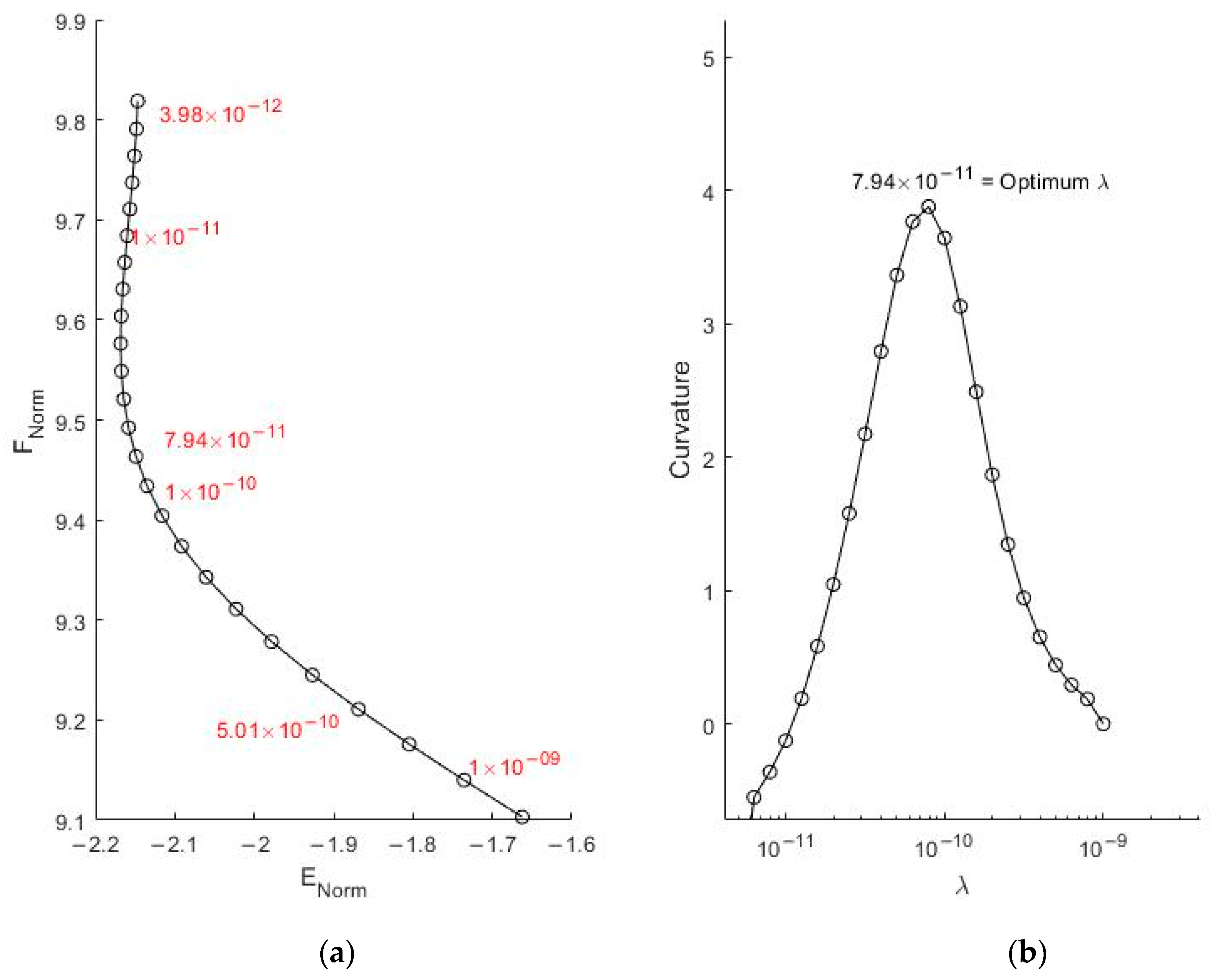
An illustrative baseline example is considered of a single 18 t vehicle travelling across the bridge on a Class A road profile at a speed of 25 m/s. Tikhonov Regularization requires a plot of the residual norm against the smoothing norm (Figure 2a), from which the point of maximum curvature is extracted (Figure 2b). In this case, that point corresponds to a value, λ = 7.94 × 10⁻⁹ (see Equation (21)), which is deemed to be the optimal trade-off between an ill-conditioned solution to the original problem and a well-conditioned solution to a slightly different problem. In Figure 2a, the x-axis represents the residual norm of the error and the y-axis denotes the smoothing norm of the regularised solution. In Figure 2b, the y coordinate represents the curvature at a specific value of λ in the L curve.
Using the optimum λ value, the force history is calculated for each axle and compared to the actual force histories, available from the forward problem calculation, in Figure 3. The bridge is present from x = 0 to 20 m and the distance between the two axles is 5 m. It can be seen in Figure 3 that, while the first axle enters the bridge at x = 0 m, the second does not arrive until x = 5 m. Similarly, the first axle leaves the bridge at x = 20 m and the second at x = 25 m. It can be seen in Figure 3 that, for this idealized case, the calculated axle forces match the real ones reasonably well. This is especially true in the context of bridge Weigh-in-Motion theory, where many systems are at, or less than, Class B accuracy, i.e., 95% of axle forces within ±15% of the exact values [45]. It can be seen in Figure 3 that the difference between the real and calculated axle forces increases when the second axle enters the bridge span. The sum of the averages of the two calculated axle force histories gives a calculated GVW of 17.84 t which, when compared to the actual GVW of 18 t, is an error of less than −1%. It should be noted that the error is calculated by (inferred-real)/real. The results of this simulation demonstrate that this new A-MFI algorithm has the potential to estimate GVW with good accuracy.

3.3. Sensitivity Study

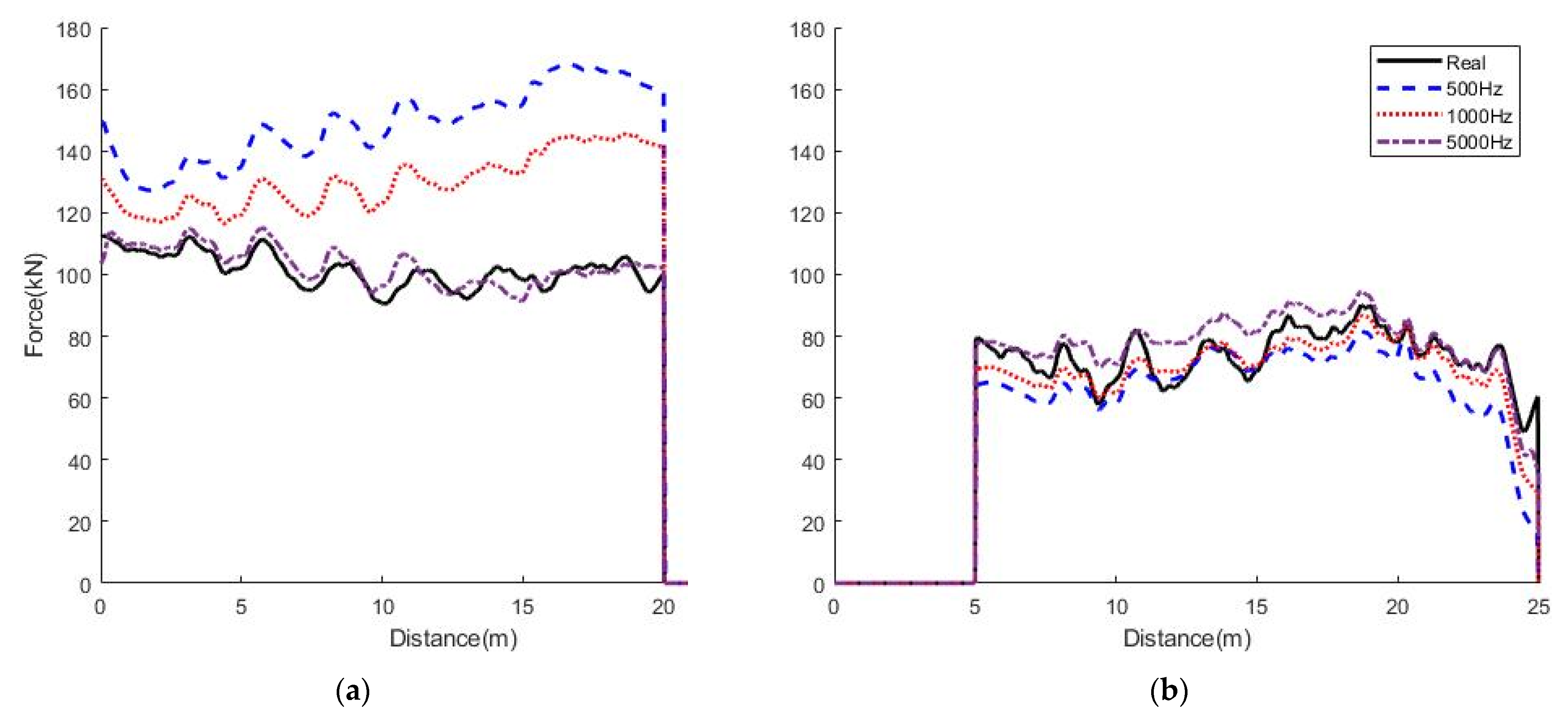
A sensitivity study was undertaken on the scan rate of the acceleration signal, inaccurate measurement of vehicle velocity, initial bridge conditions, and signal noise. The scan rate of an accelerometer dictates the frequency of measured accelerations. Linear interpolation can be used to artificially increase the sampling rate between successive scans, i.e., the number of points of calculation. While this does not provide any new information, it has significant numerical benefits in the A-MFI algorithm. For the same example from Figure 3, it can be seen in Figure 4a that the accuracy of the force history improves significantly with increasing sampling rate—with a very good match to the actual Axle 1 force history at a rate of 5000 Hz. However, there is an inaccuracy in the early parts of the Axle 2 force history in Figure 4b, which is not improved by increasing the sampling rate. Nevertheless, the average forces tend to be closer to the actual average forces and to the axle weights, as the sampling rate is increased. For this example, the calculated GVW reduces from a 21% error at a sampling rate of 500 Hz to 2.7% at a rate of 5000 Hz.
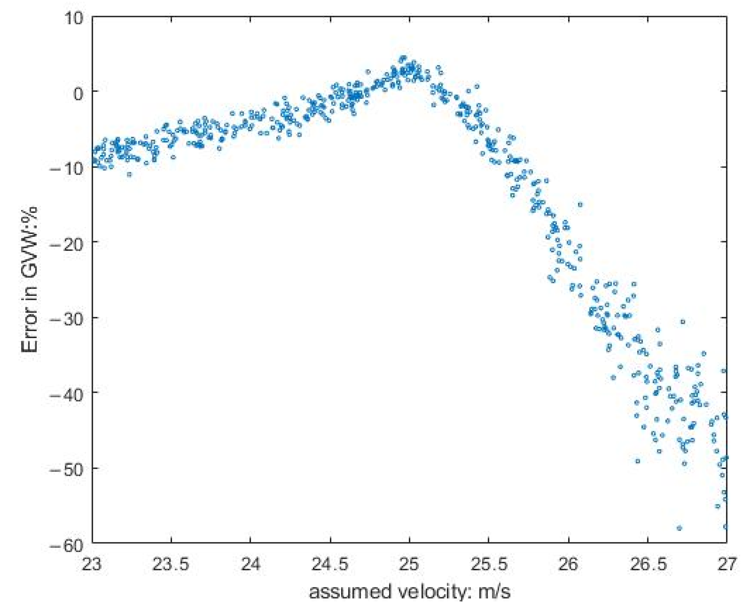
When the input velocity is not accurately measured, the accuracy of the A-MFI results is affected. Again, simulations are carried out for the baseline 18 t half-car model travelling at a constant velocity of 25 m/s and giving an error in the calculated GVW of 2.7% when the correct velocity is used in the calculation. The errors that result from inaccurate speeds are found to be −8.9%, −4.4%, −13.0%, and −49.5% for ‘measured’ speeds of 23, 24, 26, and 27 m/s, respectively. Clearly, the accuracy is greatly influenced by the assumed speed, particularly when it is higher than the actual value.
To investigate the repeatability of this effect, the analysis was run for a population of 500 vehicles (all 18 t half-cars with 25 m/s real velocity) on a Class A profile. The velocity used as the input was randomly selected within the range of 23 m/s to 27 m/s (+/− 8% error). The errors in inferred GVWs are illustrated in Figure 5 and confirm the general trend of the previous example.
One of the assumptions of A-MFI is that the bridge is stationary when the first axle arrives, a condition that is not satisfied if the test vehicle is preceded by another. To test the implications of pre-existing bridge vibration, another half-car vehicle is run over the bridge before the test half-car arrives. The test vehicle is assumed to enter the bridge at time, δt = 0.2, 0.5, 1, and 2 s after the first vehicle leaves–see Figure 6. When the vehicles are close to each other, the effect is significant. For this example, the error in the inferred GVW is −7.1% and 7.3% for δt = 0.2 s and 0.5 s respectively. However, it should be noted that this implies a headway of 1.2 s which is small relative to most recorded gaps [46]. For the larger time intervals of 1 and 2 s, the GVW errors fall to 2.3% and −0.7% respectively.
The influence of random signal noise on the accuracy of the inferred GVW is also investigated. For this example, noise of up to 5% results in GVW errors of up to about 5%, with no clear correlation between accuracy and level of noise.

4. Inferred Weight as an Indicator of Structural Health

While A-MFI may not determine the weight of a particular vehicle accurately, the results are consistent. It is well known that the mean weight for vehicles of a given class, is highly repeatable at a given site (see, e.g., [47]). Hence, if the calculated mean GVW at a site increases, it suggests a loss of stiffness, i.e., damage, in the bridge. This concept is explored in the following sections.

4.1. A-MFI Result with Damaged Bridge Case

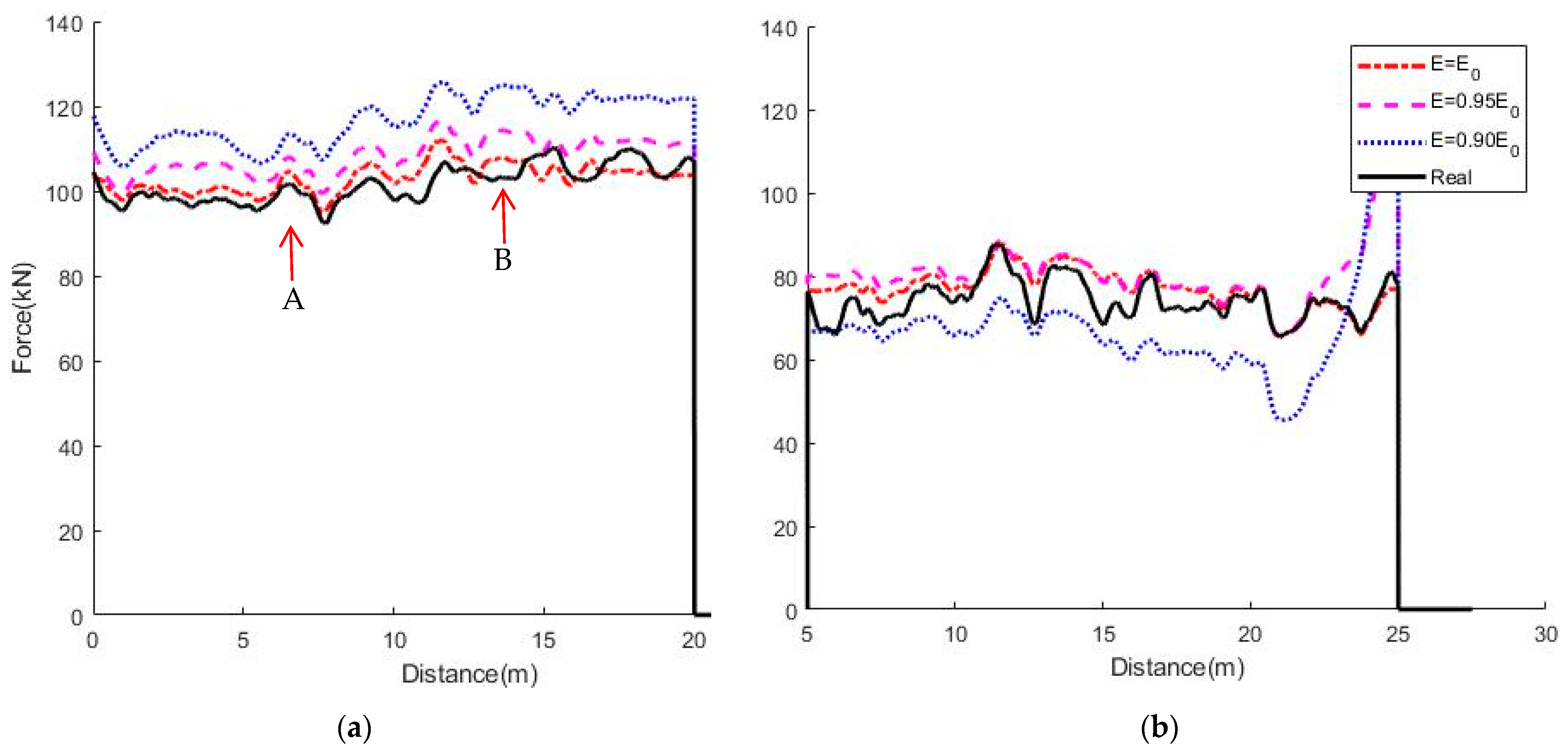
In this paper, damage in the bridge is defined as global damage with a uniform reduction of material stiffness. To investigate global damage using changes in inferred GVWs, the baseline 18 t half-car model passing at 25 m/s on a Class A profile is considered once more. Initially, different levels of global damage (reduction in Young’s Modulus) in the bridge are considered, namely, 5%, 10%, and 20%. The resulting inferred force histories for 5% and 10% only are shown in Figure 7. It can be seen that some peak forces, such as Point A in Figure 7a, are the same in the exact force history and in the A-MFI inferred force histories, regardless of damage. Other peaks, such as Point B, are present in the inferred force histories but not in the real force history. In general, the shape of the inferred force histories is not affected by these uniform levels of damage—broadly the same peaks and troughs are evident in each history.
Table 3 shows some typical results. Counterintuitively, the mean inferred GVW results increase initially (for 5% and 10% damage) but fall, as expected, for the higher damage level (20% damage). In general, the trend is counterintuitive, i.e., mean GVW tends to decrease as the damage level increases.

4.2. Bridge Damage Detection Using Inferred Vehicle GVW Statistics

Figure 8a shows the histogram of inferred weights for the healthy bridge. Figure 8b presents the histogram of inferred GVW for a population of 500 vehicles crossing the bridge for various levels of damage. Figure 8 represents ideal conditions with none of the sources of error outlined in Section 3.3 included. While the force histories and the inferred GVW for individual vehicles are inaccurately inferred, there is an underlying trend for inferred weight to decrease with increasing bridge damage (Figure 8b). This may be explained by a poor match between measured data from the damaged bridge and the theoretical equivalent healthy bridge. While there are significant inaccuracies for individual vehicles, a Normal distribution fit to the inferred vehicles is an excellent match with the Normal distribution fit to the true weights. Figure 8b shows that this distribution is visibly and consistently affected by bridge damage, even for very low damage levels. In general, bridge damage causes the peak to reduce, the standard deviation to increase, and, in most cases, the mean to shift slightly to the left.
Table 4 confirms the increasing trend in standard deviation (STD) with damage and the slight falling trend in mean inferred GVW. The trend in the mean is not fully consistent—there is a slight increase between healthy and 2.5% damage, followed by falls between 2.5%, 5%, 7.5%, and 10%.
The trends are less consistent when the results are repeated, considering various sources of potential inaccuracy. In particular, in this case, a different batch of 500 vehicles is used for each damage level, thus allowing for the natural GVW variability in the vehicle population. Table 5 summarizes the various sources of simulated inaccuracy, and Figure 9 shows the resulting statistical distributions of inferred weight. The increasing standard deviation with damage is again evident, and the slight downward trend in the mean—see Table 4.
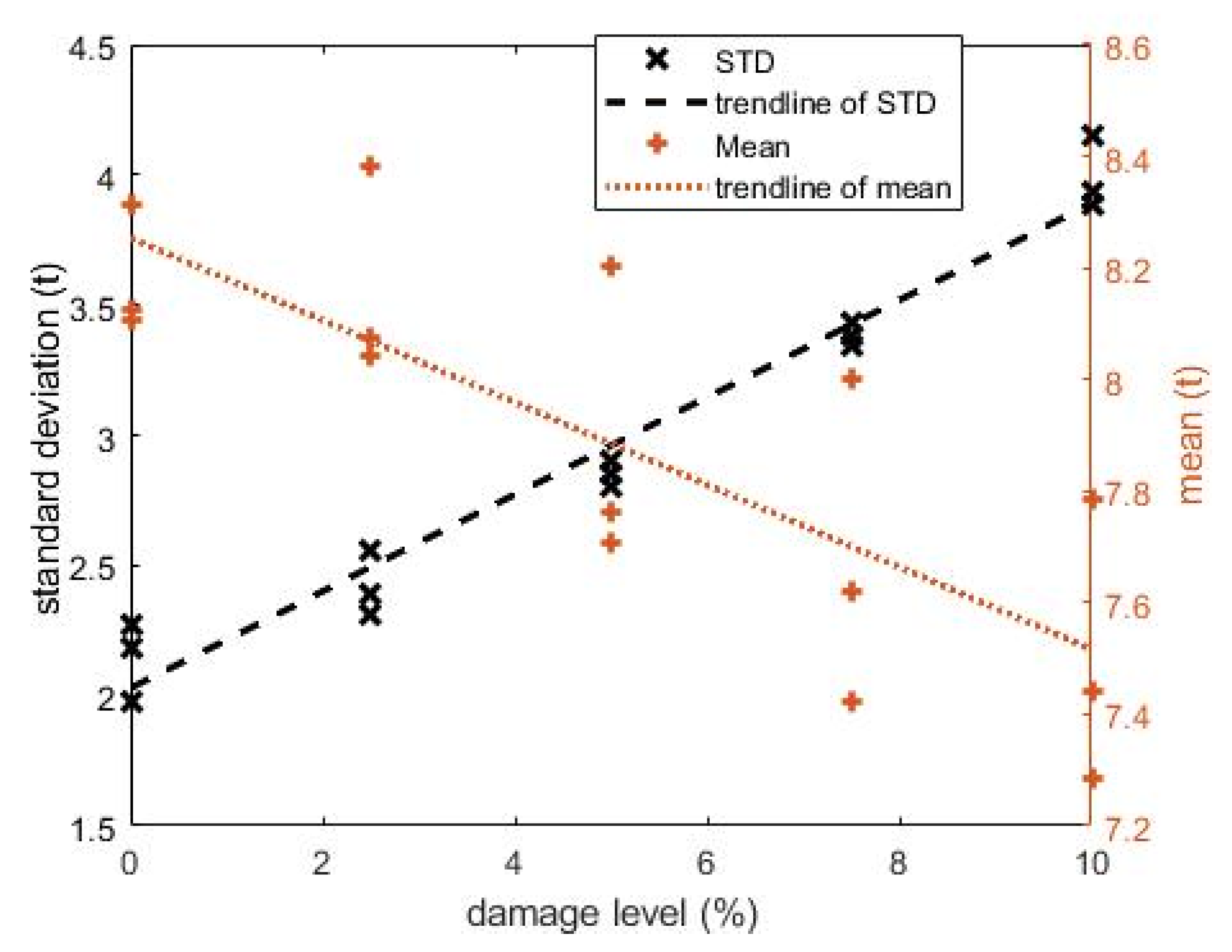
This entire set of simulations, including errors, has been carried out three times to establish the repeatability of the trends. The variations in the means and standard deviations with damage are presented in Figure 10. There is considerable variation in the inferred mean weights—the coefficient of determination (R2) of the trendline (linear regression) is only 0.63. While the general linear trend is clear, the mean inferred GVW does not always decrease with increasing damage. It is also noteworthy that, even for the healthy bridge, the mean GVWs are less than the true mean values which are 8.11 t, 8.31 t, and 8.12 t for Batches 1 to 3, respectively. This appears to be due to the simulated errors in the velocity: when the true velocities are used in the inference of healthy bridge GVWs, the results are 8.80 t, 8.91 t, and 8.95 t, respectively.
The results for the standard deviations are much more repeatable—in this case, the coefficient of determination (R2) of the trendline (linear regression) is 0.96. The variability between batches is considerably less and, for all permutations, the standard deviation of GVW increases with increasing damage. Further, the errors in velocity do not significantly affect the standard deviations for the healthy bridge—compare inferred results of 2.18 t, 1.98 t, and 2.27 t with results for perfect velocities of 2.13 t, 1.90 t, and 2.00 t, respectively.

5. Conclusions

This paper presents a newly developed acceleration-based MFI (A-MFI) algorithm, that reformulates existing MFI theory to allow, for the first time, directly measured acceleration data to be used (refer to Equations (19) and (20)). This reformulation of the underlying MFI equations allows the new A-MFI algorithm to be directly applied to acceleration data, which is damage sensitive. The accuracy of the inferred axle forces and vehicle weights using A-MFI is reasonable in ideal conditions but is found to be quite sensitive to several sources of error, particularly the accuracy of the vehicle velocity data used. Consequently, the statistics of the inferred weight are not accurate. However, the statistics are consistent, and the standard deviation of inferred gross vehicle weight is shown to correlate well with the stiffness reduction (damage level) of the bridge, even for relatively low levels of global damage.

Author Contributions

Conceptualization, methodology, formal analysis, S.W., E.J.O. and D.P.M.; software, S.W.; validation, S.W.; writing—original draft preparation, S.W.; writing—review and editing, S.W., E.J.O. and D.P.M.; supervision, E.J.O. and D.P.M. All authors have read and agreed to the published version of the manuscript.

Funding

This research was funded by the joint scholarship between University College Dublin and Chinese Scholarship Council, grant number is ‘201908300011’.

Institutional Review Board Statement

Not applicable.

Informed Consent Statement

Not applicable.

Data Availability Statement

All of the data reported in the paper are presented in the main text. Any other data will be provided on request.

Acknowledgments

The authors wish to acknowledge the financial support received from University College Dublin and Chinese Scholarship Council. The authors also gratefully acknowledge the Federal Highway Administration and the Long-Term Pavement Performance Program for access to WIM data.

Conflicts of Interest

The authors declare no conflict of interest.

Appendix A

To calculate [R]n, {S}n, [H]n and [D]n, a backward sweep process is used. For j = n,
[ R ] n = [ Q ] T [ W ] [ Q ]
{ S } n = 2 [ Q ] T [ W ] { d } n
[ H ] n = 2 [ T ] T [ R ] n
[ D ] n = [ 2 [ B ] + 2 [ T ] T [ R ] n [ T ] ] 1
Start from j = n − 1 to 1.
[ R ] j 1 = [ Q ] T [ W ] [ Q ] + [ M ˜ ] j 1 T ( [ R ] j [ H ] j T [ D ] j [ H ] j / 2 ) [ M ˜ ] j 1
{ S } j 1 = 2 [ Q ] T [ W ] { d } j 1 + [ M ˜ ] j 1 T ( [ I ] [ H ] j T [ D ] j [ T ] T ) { S } j
[ H ] j 1 = 2 [ T ] T [ R ] j 1
[ D ] j 1 = [ 2 [ B ] + 2 [ T ] T [ R ] j 1 [ T ] ] 1
The forward sweep starts from j = 1 to n:
{ X ˜ } j = [ M ˜ ] { X ˜ } j 1 + [ T ] { r } j 1
{ r } j = [ 2 [ B ] + 2 [ T ] T [ R ] j + 1 [ T ] ] 1 { [ T ] T { S } j + 1 + 2 [ T ] T [ R ] j + 1 [ M ˜ ] j { X ˜ } j }

References

  1. Farrar, C.R.; Doebling, S.W.; Nix, D.A. Vibration–based structural damage identification. Philos. Trans. R. Soc. A: Math. Phys. Eng. Sci. 2001, 359, 131–149. [Google Scholar] [CrossRef]
  2. Worden, K.; Dulieu-Barton, J.M. An Overview of Intelligent Fault Detection in Systems and Structures. Struct. Health Monit. 2004, 3, 85–98. [Google Scholar] [CrossRef]
  3. Carden, E.P.; Fanning, P. Vibration Based Condition Monitoring: A Review. Struct. Health Monit. 2004, 3, 355–377. [Google Scholar] [CrossRef]
  4. Gattulli, V.; Cunha, A.; Caetano, E.; Potenza, F.; Arena, A.; Di Sabatino, U. Dynamical models of a suspension bridge driven by vibration data. Smart Struct. Syst. 2021, 27, 139. [Google Scholar]
  5. Kim, J.-T.; Ryu, Y.-S.; Cho, H.-M.; Stubbs, N. Damage identification in beam-type structures: Frequency-based method vs. mode-shape-based method. Eng. Struct. 2003, 25, 57–67. [Google Scholar] [CrossRef]
  6. Cantero, D.; Gonzalez, A. Bridge Damage Detection Using Weigh-in-Motion Technology. J. Bridg. Eng. 2015, 20, 04014078. [Google Scholar] [CrossRef] [Green Version]
  7. Moses, F. Weigh-in-Motion System Using Instrumented Bridges. Transp. Eng. J. ASCE 1979, 105, 233–249. [Google Scholar] [CrossRef]
  8. Lydon, M.; Taylor, S.E.; Robinson, D.; Mufti, A.; Brien, E.J.O. Recent developments in bridge weigh in motion (B-WIM). J. Civ. Struct. Health Monit. 2015, 6, 69–81. [Google Scholar] [CrossRef] [Green Version]
  9. Ojio, T.; Carey, C.H.; O’Brien, E.J.; Doherty, C.; Taylor, S.E. Contactless Bridge Weigh-in-Motion. J. Bridge Eng. 2016, 21, 04016032. [Google Scholar] [CrossRef] [Green Version]
  10. Dong, C.-Z.; Celik, O.; Catbas, F.N.; OBrien, E.J.; Taylor, S. Structural displacement monitoring using deep learning-based full field optical flow methods. Struct. Infrastruct. Eng. 2020, 16, 51–71. [Google Scholar] [CrossRef]
  11. Mohammed, Y.M.; Uddin, N. Acceleration-based bridge weigh-in-motion. Bridg. Struct. 2019, 14, 131–138. [Google Scholar] [CrossRef]
  12. Sekiya, H.; Kubota, K.; Miki, C. Simplified Portable Bridge Weigh-in-Motion System Using Accelerometers. J. Bridg. Eng. 2018, 23, 04017124. [Google Scholar] [CrossRef]
  13. Park, K.-T.; Kim, S.-H.; Park, H.-S.; Lee, K.-W. The determination of bridge displacement using measured acceleration. Eng. Struct. 2005, 27, 371–378. [Google Scholar] [CrossRef]
  14. Gindy, M.; Vaccaro, R.; Nassif, H.; Velde, J. A State-Space Approach for Deriving Bridge Displacement from Acceleration. Comput. Civ. Infrastruct. Eng. 2008, 23, 281–290. [Google Scholar] [CrossRef]
  15. Sekiya, H.; Kimura, K.; Miki, C. Technique for Determining Bridge Displacement Response Using MEMS Accelerometers. Sensors 2016, 16, 257. [Google Scholar] [CrossRef] [PubMed] [Green Version]
  16. Law, S.; Fang, Y. Moving force identification: Optimal state estimation approach. J. Sound Vib. 2001, 239, 233–254. [Google Scholar] [CrossRef]
  17. OBrien, E.J.; Khan, M.A.; McCrum, D.P.; Žnidarič, A. Using Statistical Analysis of an Acceleration-Based Bridge Weigh-In-Motion System for Damage Detection. Appl. Sci. 2020, 10, 663. [Google Scholar] [CrossRef] [Green Version]
  18. González, A.; Rowley, C.; OBrien, E.J. A general solution to the identification of moving vehicle forces on a bridge. Int. J. Numer. Methods Eng. 2008, 75, 335–354. [Google Scholar] [CrossRef]
  19. Wu, S.; Law, S. Moving force identification based on stochastic finite element model. Eng. Struct. 2010, 32, 1016–1027. [Google Scholar] [CrossRef]
  20. Wu, S.; Law, S. Vehicle axle load identification on bridge deck with irregular road surface profile. Eng. Struct. 2011, 33, 591–601. [Google Scholar] [CrossRef]
  21. Chan, T.; Law, S.; Yung, T.; Yuan, X. An interpretive method for moving force identification. J. Sound Vib. 1999, 219, 503–524. [Google Scholar] [CrossRef]
  22. Law, S.S.; Chan, T.; Zeng, Q.H. Moving Force Identification—A Frequency and Time Domains Analysis. J. Dyn. Syst. Meas. Control. 1999, 121, 394–401. [Google Scholar] [CrossRef]
  23. Law, S.; Chan, T.; Zeng, Q. Moving force identification: A time domain method. J. Sound Vib. 1997, 201, 1–22. [Google Scholar] [CrossRef]
  24. Law, S.; Bu, J.; Zhu, X.; Chan, S.L. Vehicle axle loads identification using finite element method. Eng. Struct. 2004, 26, 1143–1153. [Google Scholar] [CrossRef]
  25. O’Connor, C.; Chan, T.; Tin, H. Dynamic Wheel Loads From Bridge Strains. J. Struct. Eng. 1988, 114, 1703–1723. [Google Scholar] [CrossRef]
  26. Trujillo, D.M. The direct numerical integration of linear matrix differential equations using pade approximations. Int. J. Numer. Methods Eng. 1975, 9, 259–270. [Google Scholar] [CrossRef]
  27. Trujillo, D.M. Application of dynamic programming to the general inverse problem. Int. J. Numer. Methods Eng. 1978, 12, 613–624. [Google Scholar] [CrossRef]
  28. Zhu, X.; Law, S.S.; Bu, J.Q. A State Space Formulation for Moving Loads Identification. J. Vib. Acoust. 2006, 128, 509–520. [Google Scholar] [CrossRef]
  29. Tikhonov, A.N.; Goncharsky, A.; Stepanov, V.; Yagola, A.G. Numerical Methods for the Solution of Ill-Posed Problems; Springer Science & Business Media: Berlin, Germany, 2013. [Google Scholar]
  30. Rowley, C.W.; OBrien, E.J.; Gonzalez, A.; ŽNIDARIČ, A. Experimental Testing of a Moving Force Identification Bridge Weigh-in-Motion Algorithm. Exp. Mech. 2008, 49, 743–746. [Google Scholar] [CrossRef]
  31. Carey, C.H.; OBrien, E.J.; Keenahan, J. Investigating the Use of Moving Force Identification Theory in Bridge Damage Detection. Key Eng. Mater. 2013, 569–570, 215–222. [Google Scholar] [CrossRef]
  32. OBrien, E.J.; Carey, C.; Keenahan, J. Bridge damage detection using ambient traffic and moving force identification. Struct. Control. Health Monit. 2015, 22, 1396–1407. [Google Scholar] [CrossRef] [Green Version]
  33. OBrien, E.J.; Fitzgerald, P.C.; Malekjafarian, A.; Sevillano, E. Bridge damage detection using vehicle axle-force information. Eng. Struct. 2017, 153, 71–80. [Google Scholar] [CrossRef]
  34. Trujillo, D.M.; Busby, H.R. Practical Inverse Analysis in Engineering; CRC Press: Boca Raton, FL, USA, 1997. [Google Scholar]
  35. Bellman, R. Introduction to Mathematical Theory of Control Processes; SERBIULA (sistema Librum 2.0); Elsevier: Amsterdam, The Netherlands, 1968; Volume II. [Google Scholar]
  36. Adhikari, S. Structural Dynamic Analysis with Generalized Damping Models: Analysis; John Wiley & Sons: Hoboken, NJ, USA, 2013. [Google Scholar]
  37. OBrien, E.J.; McGetrick, P.; Gonzalez, A. A drive-by inspection system via vehicle moving force identification. Smart Struct. Syst. 2014, 13, 821–848. [Google Scholar] [CrossRef] [Green Version]
  38. Keenahan, J.; Ren, Y.; OBrien, E.J. Determination of road profile using multiple passing vehicle measurements. Struct. Infrastruct. Eng. 2019, 16, 1262–1275. [Google Scholar] [CrossRef]
  39. ISO. ISO-8608: Mechanical Vibration—Road Surface Profiles—Reporting of Measured Data: International Standards Organisation; ISO: Geneva, Switzerland, 1995. [Google Scholar]
  40. Blab, R.; Litzka, J. Measurements of the lateral distribution of heavy vehicles and its effects on the design of road pavements. In Proceedings of the 4th International Symposium on Heavy Vehicle Weights and Dimensions, Ann Arbor, MI, USA, 25–29 June 1995; pp. 389–395. [Google Scholar]
  41. Walker, D.; Cebon, D. The metamorphosis of LTPP traffic data. In Proceedings of the 6th International Conference on Weigh-In-Motion (ICWIM 6) International Society for Weigh-In-MotionInstitut Francais des Sciences et Technologies des Transports, de l’Aménagement et des Réseaux (IFSTARR) International Transport ForumForum of European National Highway Research Laboratories (FEHRL) Transportation Research BoardFederal Highway Administration; Wiley Online Library: Hoboken, NJ, USA, 2012. [Google Scholar]
  42. Walker, D.; Selezneva, O.; Wolf, D. Findings from LTPP SPS WIM systems validation study. In Proceedings of the 6th International Conference on Weigh-In-Motion (ICWIM 6) International Society for Weigh-In-MotionInstitut Francais des Sciences et Technologies des Transports, de l’Aménagement et des Réseaux (IFSTARR) International Transport ForumForum of European National Highway Research Laboratories (FEHRL) Transportation Research BoardFederal Highway Administration; Wiley Online Library: Hoboken, NJ, USA, 2012. [Google Scholar]
  43. Martinez, D.; Malekjafarian, A.; OBrien, E.J. Bridge flexural rigidity calculation using measured drive-by deflections. J. Civ. Struct. Health Monit. 2020, 10, 833–844. [Google Scholar] [CrossRef]
  44. Martinez, D.; Malekjafarian, A.; OBrien, E.J. Bridge health monitoring using deflection measurements under random traffic. Struct. Control. Health Monit. 2020, 27, 2593. [Google Scholar] [CrossRef]
  45. Richardson, J.; Jones, S.; Brown, A.; Hajializadeh, D.; OBrien, E.J. On the use of bridge weigh-in-motion for overweight truck enforcement. Int. J. Heavy Veh. Syst. 2014, 21, 83. [Google Scholar] [CrossRef]
  46. Caprani, C. Calibration of a Congestion Load Model for Highway Bridges Using Traffic Microsimulation. Struct. Eng. Int. 2012, 22, 342–348. [Google Scholar] [CrossRef]
  47. OBrien, E.J.; Brownjohn, J.M.W.; Hester, D.; Huseynov, F.; Casero, M. Identifying damage on a bridge using rotation-based Bridge Weigh-In-Motion. J. Civ. Struct. Health Monit. 2021, 11, 175–188. [Google Scholar] [CrossRef]
Figure 1. Coupled vehicle-bridge system with half-car model (based on [37]).
Applsci 11 07271 g001
Figure 2. (a) L curve for 18 t vehicle passing at 25 m/s and (b) curvature of L curve vs. λ.
Applsci 11 07271 g002
Figure 3. Actual and calculated force histories for baseline example with optimum λ.
Applsci 11 07271 g003
Figure 4. Influence of sampling rate on the accuracy of A-MFI results: (a) first axle; and (b) second axle.
Applsci 11 07271 g004
Figure 5. Error in the inferred GVW due to inaccurate estimation of vehicle velocity.
Applsci 11 07271 g005
Figure 6. Schematic showing the definition of time lag (δt) between the lead vehicle departure and following vehicle arriving on the bridge (V = speed).
Applsci 11 07271 g006
Figure 7. MFI results with 5% and 10% global damage levels for; (a) first axle; and (b) second axle.
Applsci 11 07271 g007
Figure 8. Inferred GVWs for 500 vehicles: (a) Histogram for healthy and fitted Gaussian distributions of inferred and true vehicle weights; (b) fitted Gaussian distributions for healthy and damaged bridges.
Applsci 11 07271 g008
Figure 9. Gaussian curves for batches of 500 inferred GVWs with various sources of inaccuracy.
Applsci 11 07271 g009
Figure 10. Statistics of 15 batches of 500 vehicles, with simulated errors.
Applsci 11 07271 g010
Table 1. Properties of bridge model.
Span20 m
Number of finite elements20
Total degrees of freedom42
Young’s Modulus, E3.5 × 1010 N/m2
Cross sectional area 2.046 m2
Second moment of area, J0.2991 m4
Damping, ξ3%
Table 2. Vehicle population properties.
PropertySymbol/UnitsMean Value/ValueStandard Deviation
Body massms: kgFrom database
Unsprung massesMu,1: kg1100300
Mu,2: kg700250
Suspension stiffnessesKs,1: N/m0.4 × 1060.1 × 106
Ks,2: N/m1 × 1060.3 × 106
Suspension dampingCs,1: Ns/m10 × 1032.5 × 103
Cs,2: Ns/m20 × 1035 × 103
Tire stiffnessesKt,1: N/m1.75 × 1060.5 × 106
Kt,2: N/m1.75 × 1060.5 × 106
Axle spacingD1+ D2: mFrom database
SpeedVel: m/sFrom database
Table 3. Average axle force for different levels of damage.
Damage LevelAverage Axle 1 Force (kN)Average Axle 2 Force (kN)GVW (t)Error in Inferred GVW
0%1037718.31.9%
5%1088119.37.0%
10%1176718.84.3%
Actual1027417.9−0.58%
Table 4. Inferred GVW statistics for different damage levels.
Accurate MeasurementsMeasurements with Various Sources of Inaccuracy in Table 5 (% Error in Brackets *)
Damage levelSTD (t)Mean (t)STD (t) Mean (t)
Actual1.86 8.771.949.06
0%2.07 8.68 2.27 (17%)8.12 (−10%)
2.5%2.18 8.71 2.55 (31%)8.04 (−11%)
5%2.718.49 2.89 (49%)7.71 (−15%)
7.5%3.458.17 3.34 (72%)7.42 (−18%)
10%4.147.92 3.88 (100%)7.28 (−20%)
* Note: numbers in the brackets are the percentage difference from true value.
Table 5. Variables in simulation.
Number of Vehicles Per Batch500
Batches of vehicles
Velocity error (mean, std) (%)
Randomly chosen from WIM database
(0%, 3%)
Pre-existing deflection (time intervals)After first vehicle leaves bridge 0.5–2 s
Measurement noise3%
ProfileClass A, carpet profile, the same for each batch of vehicles
Publisher’s Note: MDPI stays neutral with regard to jurisdictional claims in published maps and institutional affiliations.