1. Introduction
The transportation industry plays an essential role in national economics, while vehicles may suffer downtime from spare parts being out of stock. For spare parts classification management, decision-makers should select optimal inventory strategies in terms of cost and reliability. One third of the maintenance support cost of an industrial system may be spent on stocking ample spare parts for timely maintenance [
1]. It is especially challenging to manage tens of thousands of spare parts necessary for modern industry. Thus, classification has been an important technique in the spare parts management that can support decision-makers in strategizing to allocate inventory with optimal cost and high reliability [
2,
3].
Spare parts classification has been extensively investigated by scholars [
4,
5,
6]. Different service backgrounds bring about significant differences in the criteria selection and algorithms adopted by decision-makers. Among the traditional spare parts classification methods, both ABC and VED analyses are simple and basic methods in which spare parts are arranged according to only one criterion. The ABC method was first proposed by Gelder and Van Looy [
7] and Tanwari et al. [
8] to divide spare parts into categories (A, B, and C) using total annual cost and inventory criteria. VED analysis is a simple qualitative approach to decision-making based on spare parts “criticality” as defined by experienced experts. In practice, however, they do not entirely reflect the management requirements for spare parts because a single criterion is too subjective. As proposed in 1988 [
9], a good-structured spare parts classification should be a value assessment system that requires the combination of maintenance engineers, material managers, quality control personnel, and other relevant experts. Therefore, Kraljic [
10] first proposed a second-order matrix of supply risk and criticality in view of multi-criteria, and other scholars have also applied this principle to develop new multi-criteria classification methods such as AHP (Analytic Hierarchy Process) and similar hierarchical-based analysis. Braglia [
11] proposed the Multi-Attribute Spare parts Tree Analysis (MASTA) method, which uses a decision tree and AHP to assign calculations to various criteria. Cakir and Canbolat [
12] combined AHP with fuzzy logic to capture the uncertainty in an evaluation indicator and export priority values from a judging set via fuzzy optimization. Zeng et al. [
13] proposed an algorithm that integrates AHP, fuzzy evaluation, and gray association analysis to translate qualitative descriptions into quantitative data for spare parts classification in a limited and uncertain environment. Golam Kabir [
14] also employed fuzzy AHP to determine the relative weights of attributes/criteria in a given inventory. Ng [
15] used an optimized approach to solve the weights of each criterion in a classification system—assuming that each criterion for all spare parts falls into a descending order—and finally translated the score of each spare part into a uniform scale score. Based on the Ng model, Hadi-Vencheh et al. [
16] calculated the weight of each spare parts in a system using a nonlinear optimization algorithm as the basis for the subsequent calculation of the total score. Though effective in some regards, AHP-based methods are still not well-suited to real-world spare parts classification due to the subjective matrix assignments and limited learning ability.
In order to overcome the defects in multi-criteria models regarding to weight assignment and reclassification learning ability, scholars have attempted to optimize heuristic intelligent algorithms such as Data Envelopment Analysis (DEA), Support Vector Machine (SVM), Artificial Neural Network (ANN), Genetic Algorithm (GA), Particle Swarm Optimization (PSO), gray theory, fuzzy logic, and combinations thereof. Yu [
17] compared SVM, backpropagation (BP), K-Nearest Neighbors (KNN) and other methods to find that artificial intelligence-based methods are relatively more accurate. Partovi [
18] also utilized BP and GA learning methods in ANNs for reliable, accurate inventory classification. Cai [
19] adopted an SVM based on a Kraljic three-dimensional (3D) model for enhanced quality-oriented material classification accuracy. Liu [
20] integrated a fuzzy neural network and decision tree for spare parts classification in terms of actual demand in a steel enterprise with multiple attributes. Guo [
21] constructed a novel kNN model wherein the k value can be optimized automatically to enhance the efficiency and accuracy of classification. Models based on intelligent or heuristic algorithms can process high-latitude and nonlinear sample data, but lack the rules explanatory in a degree.
Thus, for the existing spare parts classification methods, there may be some persistent problems summarized from the following three aspects:
- (1)
Visualization: Neither multi-criteria nor traditional ANN models can provide decision-makers with intuitive, visually interpretable data.
- (2)
Rules explanatory: Data-driven artificial intelligent algorithms proceed in a “black box”, where rules are not explained and results are relatively uninterpretable, despite their certain learning ability.
- (3)
Learning ability: While there are understandable variable-selection and structure-construction processes in rule-based methods, their learning ability and generalization are relatively poor.
Therefore, a novel approach based on hierarchical classification and the Convolutional Neural Network (CNN) will be developed in this study to resolve the above problems. The proposed model combines the advantages of both hierarchical structure and CNN.
Hierarchical classification serves to construct a criteria structure based on the causal relationship of multi-criteria, which makes for an explanatory rule-setting process. Moreover, the multiple criteria are distributed on the subspace by reducing the hierarchy in order to reduce the restriction of the model on the number of criteria. As described by Hu and Wang [
22], the hierarchical structure shows the causal relationship between criteria and makes it possible to consider as many variables as demanded. Bacchetti [
23] created a hierarchical multi-criteria spare parts classification method and verified it in an Italian household appliances manufacturing company. With the constructed structure, the criteria can be colored for specific data features, which transfers the classification into an image-identification problem.
The CNN is a deep learning method [
24,
25,
26] for image identification and classification, and several networks based on CNN have been explored in the past years, such as LeNet, AlexNet, VGG (Visual Geometry Group)-Net, ResNet and DenseNet. Wang [
27] proposed a CNN-based symbolic hierarchical cluster method for operation trend prediction problems, where the CNN structure is used to classify trends. Ren [
28] used AlexNet to classify different disturbances in a 3D-printing heating map process. All developed networks from CNN have their own excellent specifics. The core of ResNet model is to establish skip connection between the front layer and the back layer, which is helpful in relieving the gradient problem by residual fitting in the back propagation of training process [
29]. DenseNet is mainly distinctive in the dense connection and feature reuse that improve the calculation capacity [
30]. However, AlexNet is a deep CNN structure which can solve gradient problem better with the Relu function. Additionally, both dropout and GPUs (Graphics Processing Units) technology are adopted to improve the calculation capacity when considering the overfitting problem [
31].
This paper is organized as follows:
Section 2 introduces the deep CNN principle, which is the basis of the proposed algorithm. The proposed G-DCNN method and its stepwise operation process are presented in
Section 3.
Section 4 reports the case study conducted to validate the proposed method, as well as a comparison between the proposed method and other similar methods.
Section 5 gives a summary, concluding remarks, and a brief statement regarding future research directions.
2. Preliminaries
The deep CNN used in this study is called AlexNet, which has a structure first proposed in 2012 by Alex Krizhevsky. The overall structure of the AlexNet network is similar to that of LeNet. Both networks are convolved first and then fully connected, though the details are rather different.
2.1. Convolution Layer
Convolution operation is the most important link in the CNN structure. Local features with different dimensions are obtained using different convolutional kernels. The convolution layer has three parts: convolutional calculation, residual calculation, and gradient calculation.
2.1.1. Convolutional Calculation of the Convolution Layer
Assuming that the
layer is the convolutional layer and the
layer is the subsampling layer, the
feature map of the
layer can be calculated as follows:
where
is the feature map,
is the convolutional kernel,
is the bias, and
is the convolutional operation.
2.1.2. Residual Calculation of the Convolution Layer
Subsampling layers are always placed after the convolutional layer. A one-to-one non-overlapping sampling method is adopted. The residual of
feature map of the
layer can be expressed as follows:
where
is the residual,
is equal to the “weight” defined at a downsampling layer map,
is the output activation function,
is the output of the certain layer,
is the element-wise multiplication, and
is an upsampling operation.
2.1.3. Gradient Calculation of the Convolution Layer
Gradient descent calculation can provide the minimum loss function and model parameter values. The derivation of the bias
is:
where
is the error and
is the position of the output convolution map. The derivation process of the kernel
is:
where
is the patch, which is multiplied elementwise by the kernels during convolution.
2.2. Subsampling Layer
The subsampling layer (also called the “pooling layer”) is operated similarly to the convolutional layer. However, the convolution kernels of the subsampling layer only take the maximum value or average value of the corresponding position; the subsampling layer does not take any modification due to BP into consideration either.
2.2.1. Convolution Calculation of the Subsampling Layer
Assuming that the
layer is the subsampling layer, the
layer is the convolution layer, and the sampling size is 2
2, the convolution process can be described as follows:
where
represents the sum of the 2
2 size of the previous convolutional layer. The results are multiplied by the weight
and the activation function is applied after adding the bias.
2.2.2. Residual Calculation of the Subsampling Layer
The residual calculation formula used here is constructed in MatLab.
where
represents rotating the kernel to make the convolution function perform cross-correlation, ′
′ is the convolution operation, and ′
′ is the full convolution process.
2.2.3. Gradient Calculation of the Subsampling Layer
The bias
derivation process of the subsampling layer is the same as the convolution layer. The weight
derivation process is:
2.3. AlexNet Structure
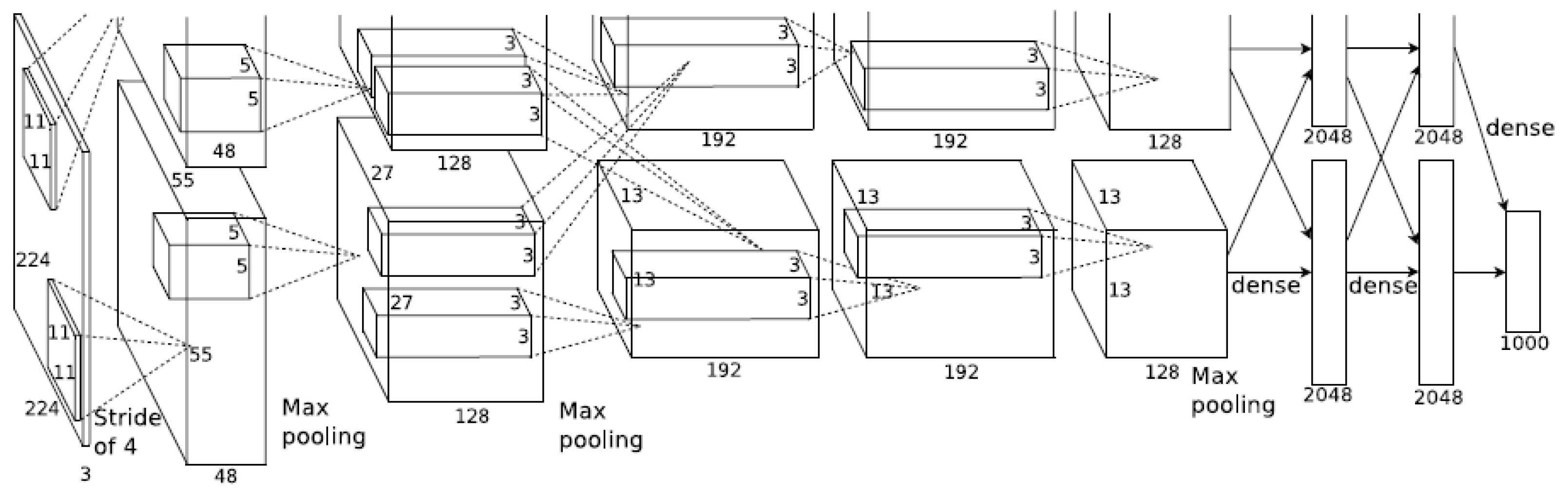
For original AlexNet structure, as shown in
Figure 1, there are a total of eight layers including five convolutions and three fully connected layers in this network. It is obvious that the AlexNet structure proceeds in both the upper and the down layer with 2GPUs at the same time, which improves the computing efficiency greatly [
32].
The first layer is the input layer wherein RGB images with pixels of 224 × 224 × 3 are preprocessed into 227 × 227 × 3. In this layer, 96 convolution kernels 11 11 3 in size are used to extract the features. With the stride movement of four pixels, FeatureMap generates 55 × 55 × 96. FeatureMap is input into the first ReLu activation function and then processed via max-pooling with a pooling unit of size 3 3 to obtain pixel sets of 27 × 27 × 96. Local response normalization is adopted in this layer with the output 27 × 27 × 96, and the data is divided into two groups as 27 × 27 × 48 because of two GPUs.
Next, for the second layer, the input has been two sets of 27 × 27 × 48. For each set, 128 convolution kernels 5 5 48 bring about the output of 27 × 27 × 128. There are the same calculation processes in this layer as the first layer, including ReLu function and local response normalization, finally with the output of two sets 13 × 13 × 128.
The third layer is fully connected to the two GPUs in second layer. However, only convolution and ReLu are processed in this layer with 384 convolution kernels 3 3 256, with the FeatureMap of 13 × 13 × 384 and 13 × 13 × 192 for each GPU.
Same process happen in the fourth layer with the output of 13 × 13 × 192.
In the fifth layer, the input data are two sets of 13 × 13 × 192 with 128 convolution kernels of size 3 3 192. The scale of the pooling operation is 3 3, the step size of the operation is 2, and then the output of 6 × 6 × 256 is obtained.
The sixth layer is a fully connected layer with the input of 6 × 6 × 256. There are a total of 4096 filters with size of 6 6 256 that can perform convolution operations. Since the size of convolution kernel is same as the size of input, there is only one value after convolution operation. Therefore, the size of the convolution pixel layer is 4096 × 1 × 1. Namely, there are 4096 neurons. The 4096 neurons are processed by ReLu function and output 4096 values.
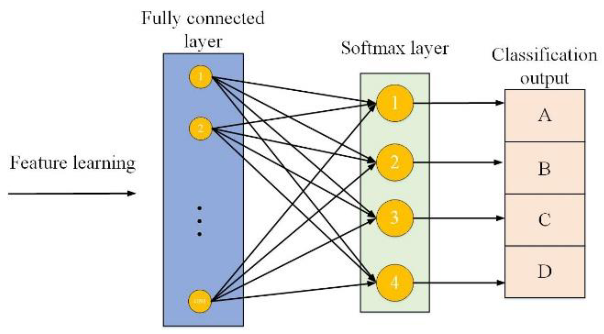
There are same fully connected, ReLu function and Dropout process in the seventh layer with the 4096 input. Finally, the 4096 data are fully connected to the 1000 neurons in the eighth layer. The probability of the 4096 data moving toward the 1000 categories can be calculated accordingly. The category corresponding to the largest probability value is selected as the category of the initial input image.
Unlike the SVM method, which has an uncalibrated computation process and scores for all classes that are not easily interpretable, the Softmax classifier allows the user to compute “probabilities” for all labels. For example, given an image, the SVM classifier might give scores [12.5, 0.6, −23.0] for the classes “cat”, “dog”, and “ship”. The Softmax classifier can instead compute the probabilities of the three labels as [0.9, 0.09, 0.01], which allows the confidence in each class to be interpreted
4. Case Study
In this section, the proposed G-DCNN model is applied and validated with a real-world case study.
4.1. Problem Description
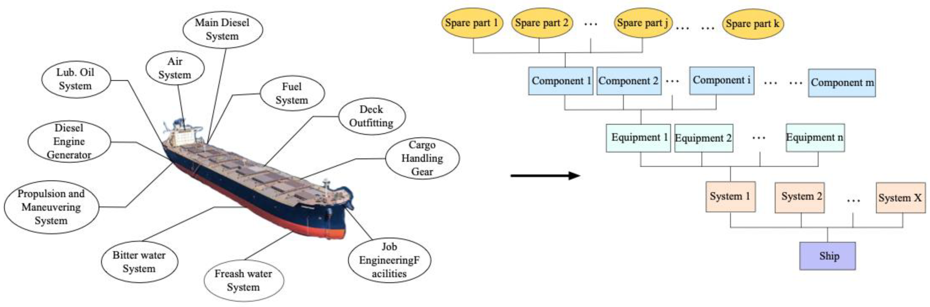
Ships are a typical long-cycle equipment system with an average life span of 30–50 years. Throughout the life cycle, they are subject to regular repairs and maintenance requiring extensive spare parts storage and supply. A regular ship has more than 10 systems consisting of 4000+ components as shown in
Figure 6. Some of the components are critical to the reliable operation but highly expensive to keep in stock at all times. It is also common for the ship to carry a large number of spare parts that may not be replaced for years.
There are a total of 73 ships served on the trading routes in this case study company, which demand vast types and huge quantities of spare parts to ensure reliable operation over the equipment’s whole life cycle. Therefore, it is essential and challenging for the shipping company to make strategic purchasing and stocking decisions according to the spare parts classes.
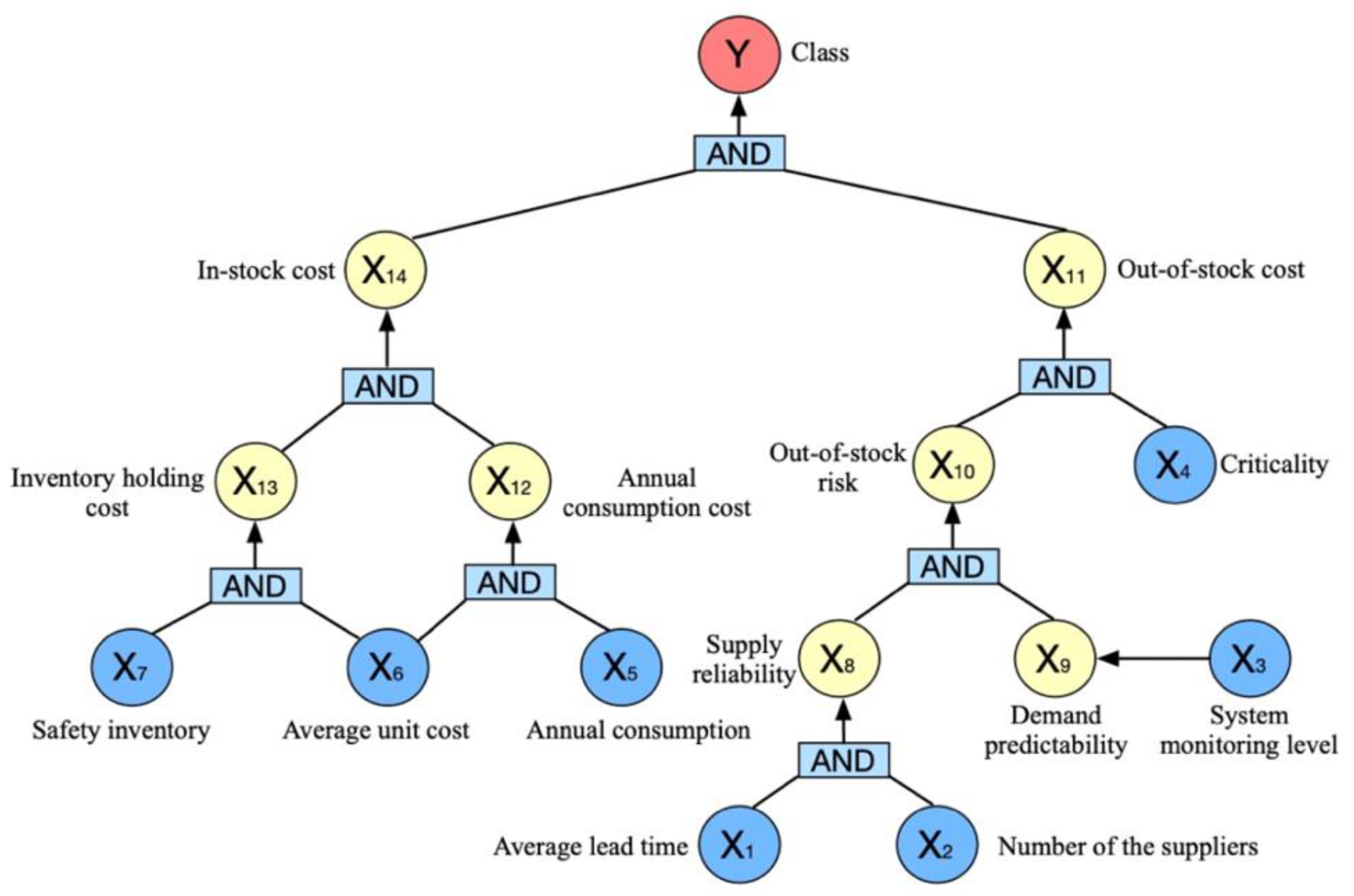
4.2. Hierarchical Structure of Ship Spare Ship Parts Classification
There are three main categories of classification criteria most commonly used in cases such as: (1) the inherent properties of the spare parts (criticality and cost); (2) consumption characteristics including failure rate and inventory turnover; (3) supply chain characteristics (lead time and supply reliability). Fourteen criteria are selected for this case study under advisement of the spare parts manager to determine the final class of spare parts: X
1 (average lead time), X
2 (number of suppliers), X
3 (system monitoring level), X
4 (criticality), X
5 (annual consumption), X
6 (average unit cost), X
7 (safety inventory), X
8 (supply reliability), X
9 (demand predictability), X
10 (out-of-stock risk), X
11 (out-of-stock cost), X
12 (annual consumption cost), X
13 (inventory holding cost), X
14 (in-stock cost).
Table 1 provides further description of the 14 criteria.
All the 14 criteria are collected based on expert knowledge and the literature in view of inventory, supply, and technology information. There are seven input variables in this case, as shown in
Table 1, wherein X
1 (average lead time), X
2 (number of suppliers), X
5 (annual consumption), X
6 (average unit cost), and X
7 (safety inventory) are quantitative values gained from the actual dataset while X
3 (system monitoring level) and X
4 (criticality) are qualitative values assessed by the spare parts manager based on their personal experience. The hierarchical structure of spare parts classification in the ship system is constructed here according to both causal relationship and expert knowledge. As shown in
Figure 7, the relationship of multiple criteria can be explained clearly.
For criteria, they can be scaled into different levels according to the data feature space. The original structure and distribution of criteria data for the spare parts are shown in
Table 2.
In the hierarchical structure, the variable relationship is constructed into layers and a final level emerges that is determined by the inventory cost and out-of-stock cost. The target output of hierarchical structure falls into four classes: A, B, C and D. The spare parts in class A are always highly expensive to keep in stock but are seldom needed. These out-of-stock spare parts will bring about the system heavy losses. Thus, the corresponding component is focused on closely monitoring and prognosis. The spare parts in class B are also highly expensive to keep in stock but not as much as class A, and the replacement of spare parts in class B happens more frequent. It is often strategic to decide the inventory amount of B spare parts and guarantee supplies. The spare parts in class C are always those that are used as part of normal consumption of scheduled maintenance that are ordered in regularly. They are neither expensive nor difficult to obtain when necessary. Spare parts in class D can be the daily consumption items that have little influence on the operation.
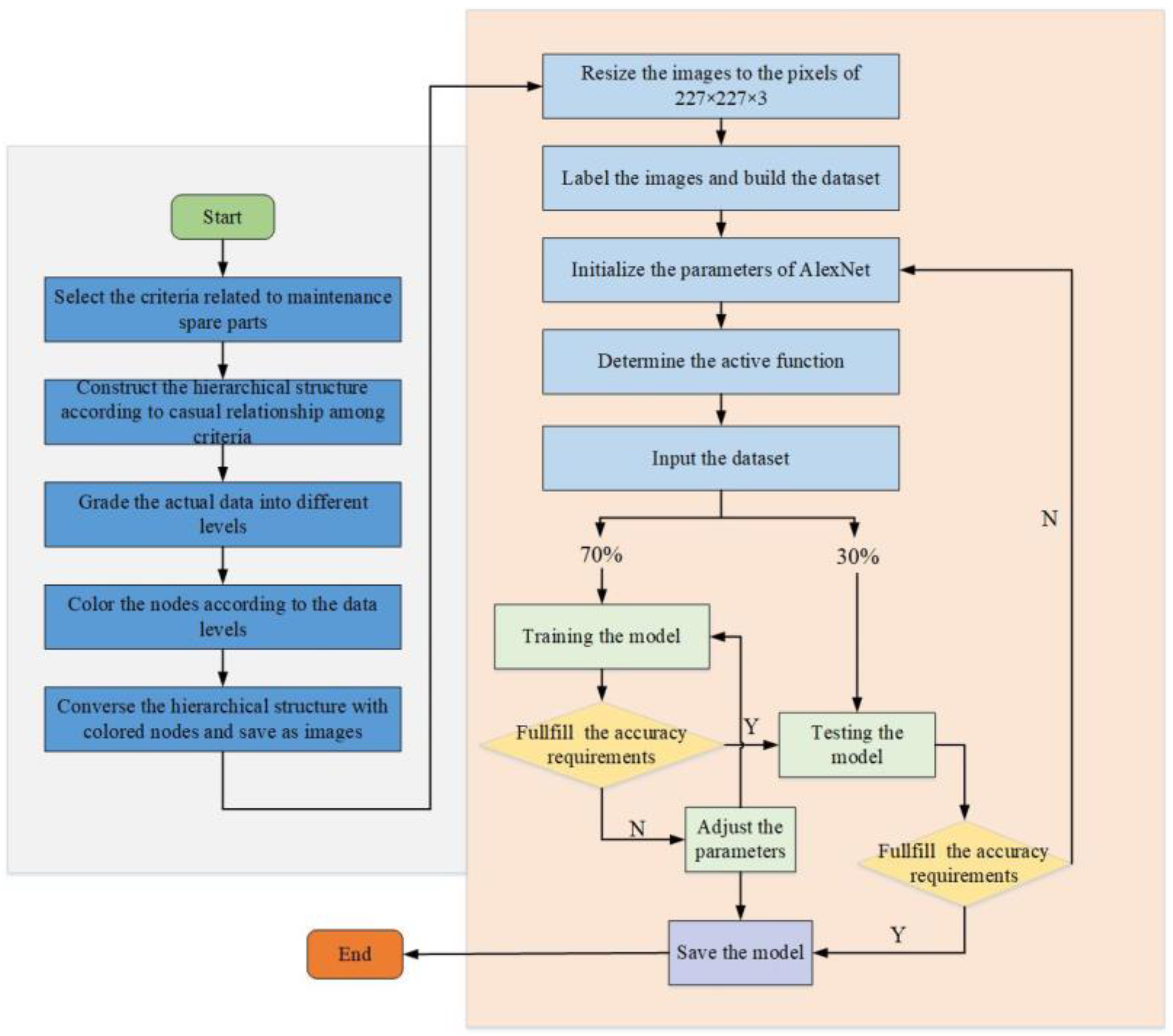
4.3. Hierarchical Classification Structure Image Conversion
To convert the spare parts classification into an image classification problem, 15 total variables involved in the hierarchical structure are represented by different colors according to their level status.
Table 3 describes the color assignments corresponding to specific criteria.
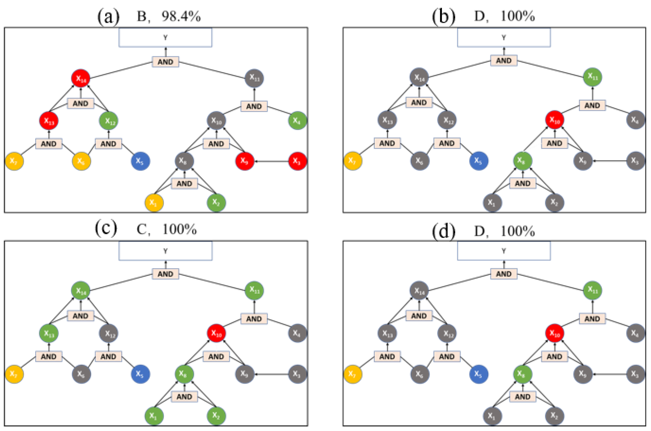
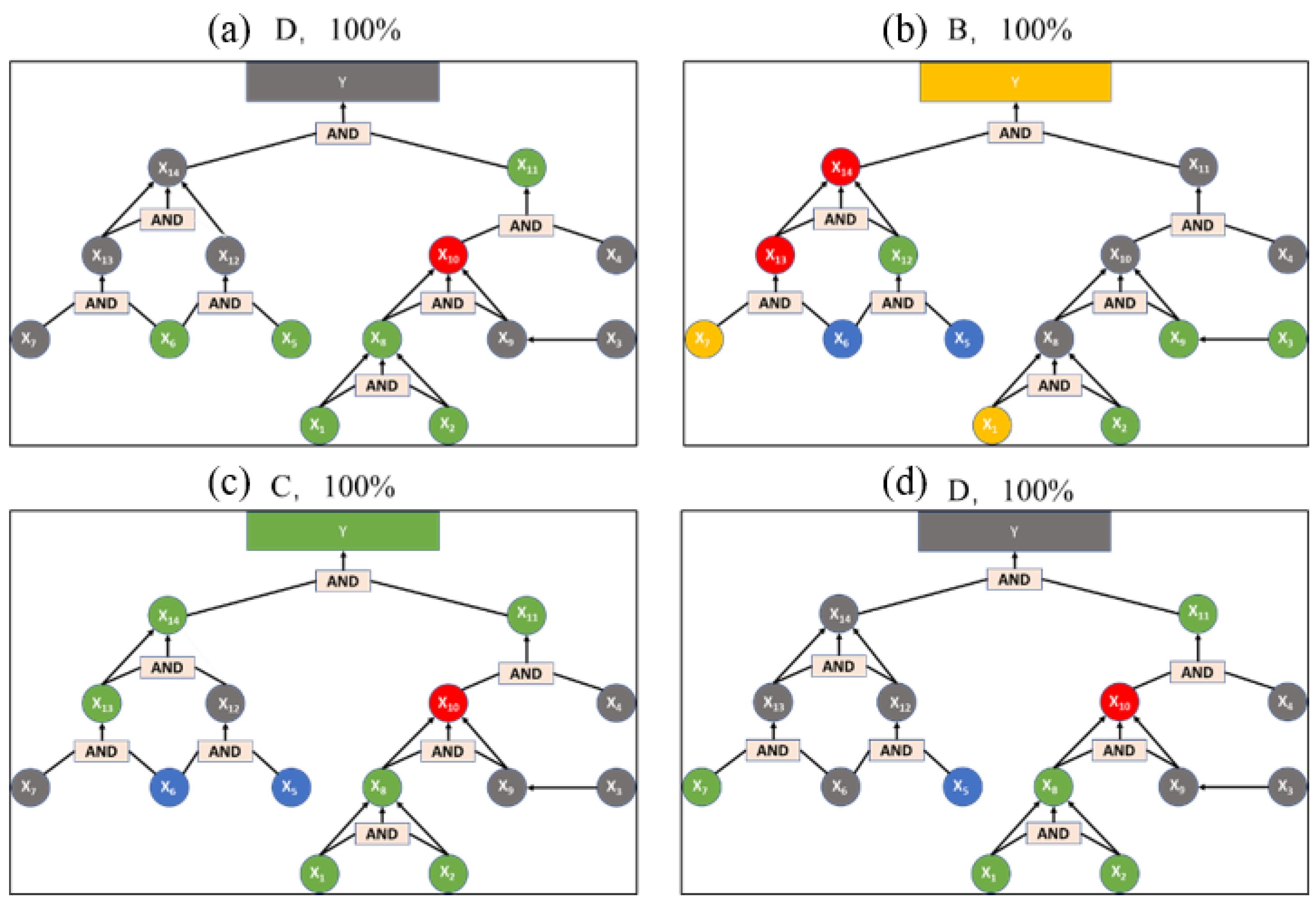
An example of spare part No. 144 (Oil temperature control valve) is given in
Table 4 and
Figure 8. All of its criteria are colored according to their actual status, the part appears to fall into class B.
4.4. Supervised Learning Analysis Based on Proposed Method
After the variables are assigned with different colors, the hierarchical structure could be updated and saved as images. In the first phrase, the learning process is conducted under a supervised environment, and the model is designed to be trained by two different datasets to determine how the sample quantity affects the results.
4.4.1. Classification Results Analysis with Few-Shot Samples
In the primary learning process, 189 labeled spare parts from the auxiliary system are selected: four from class A, 26 from class B, 43 from class C, and 116 from class D. The dataset is divided into training and testing sets.
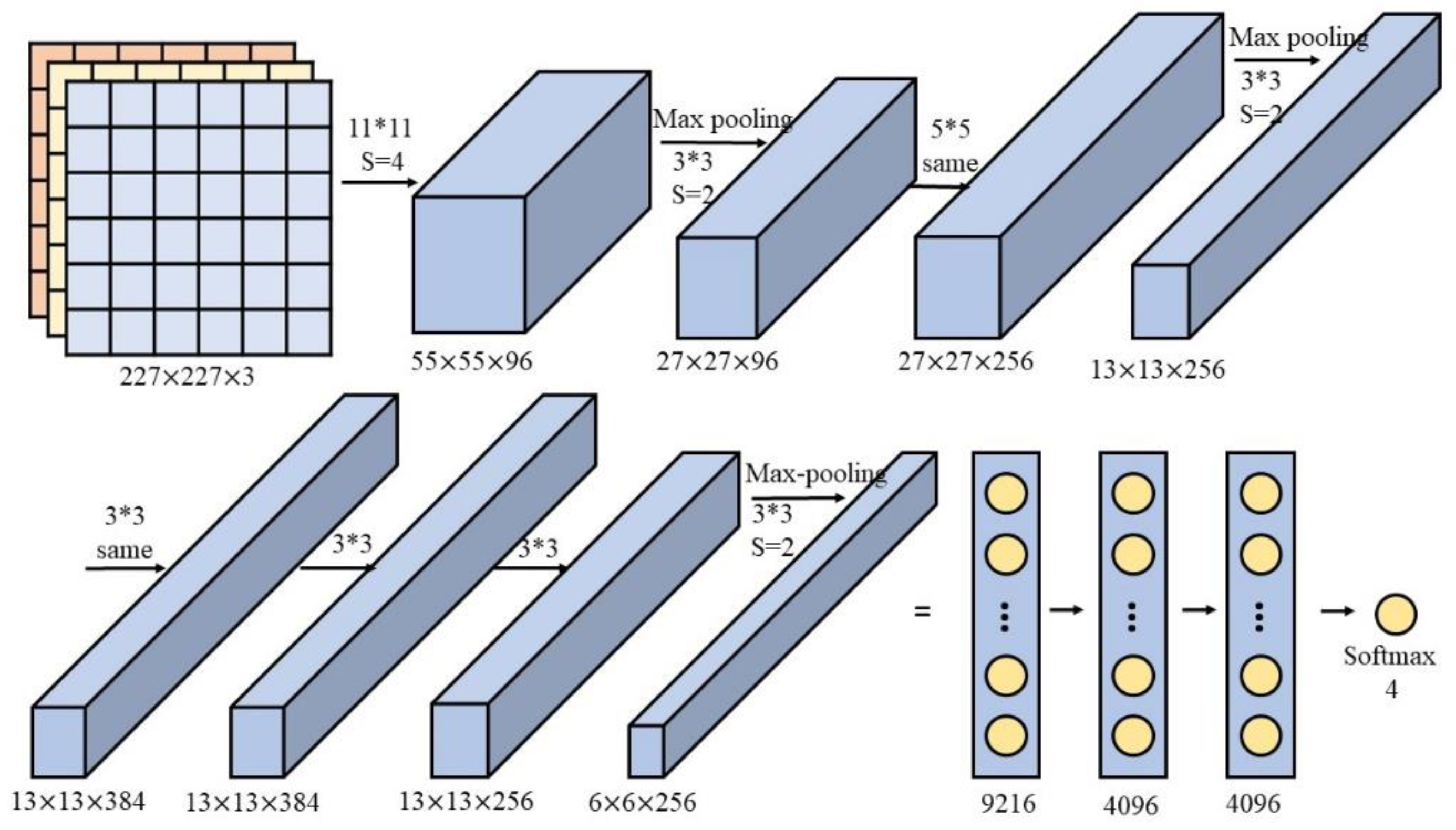
All the spare parts data are transferred into colored hierarchical structure and saved as images. Subsequently, all the images are processed in the modified AlexNet model as discussed in
Section 3.2. The modified AlexNet structure has five convolution layers and three fully connected layers. Every image is 227 × 227 in size; the ReLU activations ensure that no outputs after the convolution or fully connected layers have overfitting problems. Once the output is calculated and output by the last fully connected layer, a Softmax layer determines the final category of the image. The final classification results in this case split the images into four different classes: A, B, C, and D.
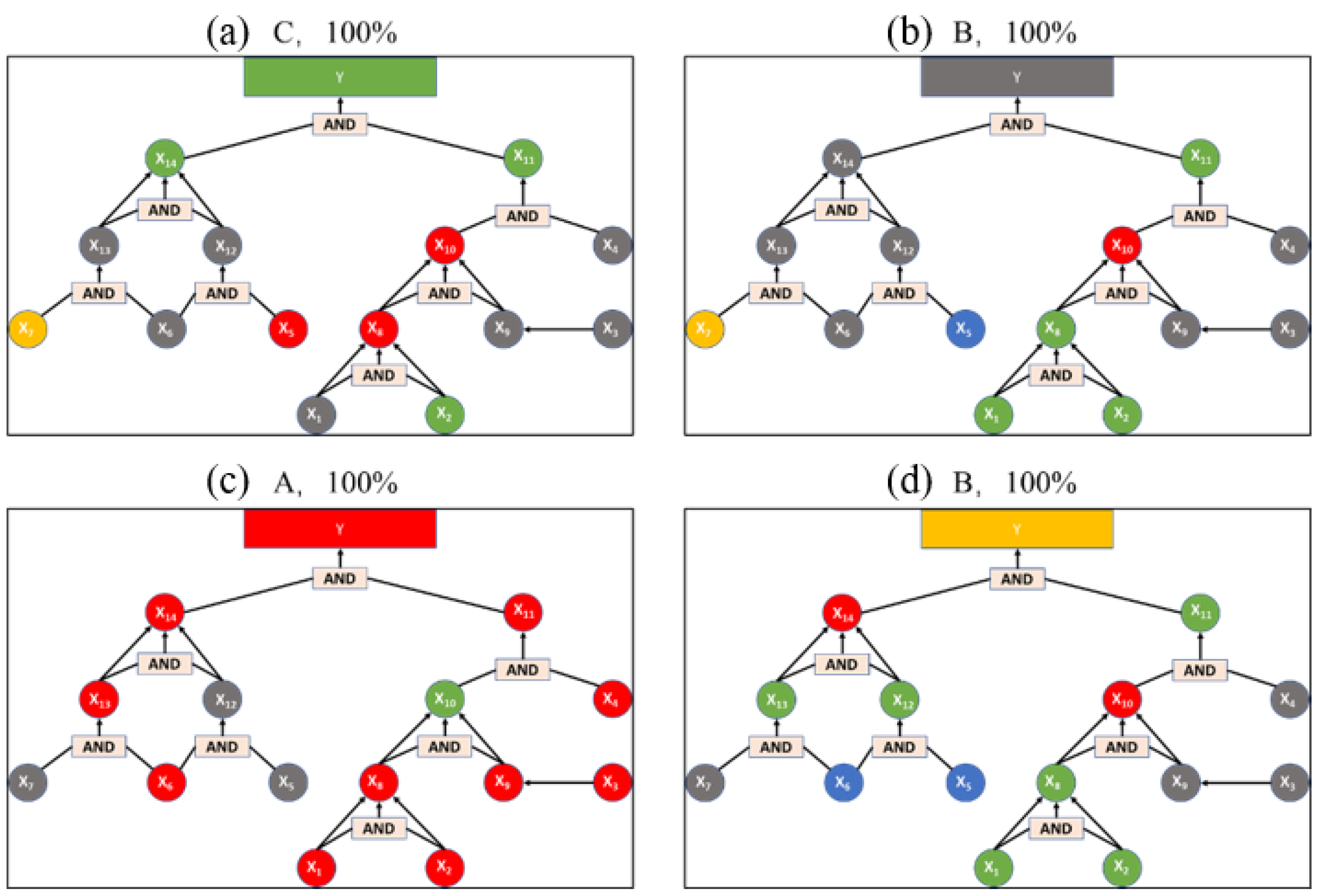
For the 189 images in this step, the first random 100 images are trained using the modified AlexNet, as shown in
Figure 9. Some of the classification results are shown in
Figure 8. It is indicated that the four results are D, B, C, D respectively. It is obvious that the listed four spare parts images are all classified with an accuracy of 100%. Additionally, for the overall training result, the average accuracy of the modified model reaches 99.8%, which can fully satisfy the practical demand.
Then, the constructed model is also used to test the remaining 89 images, and the commonly used indicator recall ratio
r and precision ratio
p are adopted to evaluate its performance:
where
is a true positive classified correctly as positive,
is a false negative misclassified as false, and
is a false positive misclassified as positive. The test accuracy of each category is determined here as follows:
where
is a true negative classified correctly as negative.
The classified results for
TP,
FP,
TN, and
FN are shown in
Table 5, and the results of
r and
p for the testing are shown in
Table 6.
For practical application in the spare parts classification, as shown in
Table 5, there is one sample in class A that is classified as false positive. It is the true spare part No. 23 that is easily classified to be A because both its unit price and annual inventory cost are high. However, in the actual management, this item is classified into B class since it is in high monitoring and the supply reliability is high.
As shown in
Table 5, the overall accuracy for B, C and D is 86.7%, 87.5% and 97.9%, respectively. However, the accuracy for class A is merely 50%, since there are only two samples in the testing set. However, when the results are analyzed with precision and recall, it indicates the modified AlexNet structure appears to perform well. Especially for class A, the recall rate is 100%, although the precision ratio is only 50%. It is obvious that
p and
r metrics contradict each other. One of the main reasons is that class A has the fewest number of training samples, which may cause an under-fitting problem in the machine learning models. Thus, for the unbalanced dataset of class A, we explore the F-measure value to assess its performance:
For class A, the value is 0.667, which can still prove the effectiveness of the model. The characteristic of the result is consistent with the fact that category A are always the most critical, expensive, and highly reliable spare parts; accordingly, these parts have limited stock, which complicates the training results in this test.
4.4.2. Re-Classified Results Analysis with Additional Samples
As mentioned above, few-shot problems emerged in the training process. Meanwhile, to consider and research the model learning ability, the samples are extended to 804 spare parts of the whole ship to cover a sufficient number of class A parts to verify the model. For the data distribution, there are 70 spare parts from class A, 122 spare parts from class B, 174 spare parts from class C, and 438 spare parts from class D. The whole spare parts are divided into two different datasets; the first 450 parts are regarded as the training set and the remaining parts as the test set. The overall training accuracy is 97% in this case. A portion of the training results are shown in
Figure 10.
The training results are acceptable. An additional test model is built using the remaining spare parts dataset. The classification results for
TP,
FP,
TN, and
FN are shown in
Table 7.
The accuracy of class A has been improved to 97.5% after these additional samples are added, while class B, C, and D maintained 100% accuracy. The G-DCNN algorithm appears to yield ideal classification results when it is applied to labeled samples.
4.5. Semi-Supervised Learning Analysis Based on Proposed Method
However, it is difficult to achieve the exact level descriptions of spare parts in practice. A semi-supervised learning analysis technique is developed based on the proposed method to verify the generality of the rules. The final color boxes of the structure are removed from the level judgment in the hierarchy to produce un-labeled samples, as shown in
Figure 11. The remaining variables are still used to test the effectiveness of the modified AlexNet algorithm in this case.
A total of 324 images are selected from all the 804 spare parts of the whole ship with a random ratio of labeled samples for further verification. A portion of the training results are shown in
Figure 12. The overall training accuracy is 95.2% in this case, which is still acceptable. Then, the selected spare parts are used to test, and the test results for
TP,
FP,
TN, and
FN in the semi-supervised learning process are shown in
Table 5.
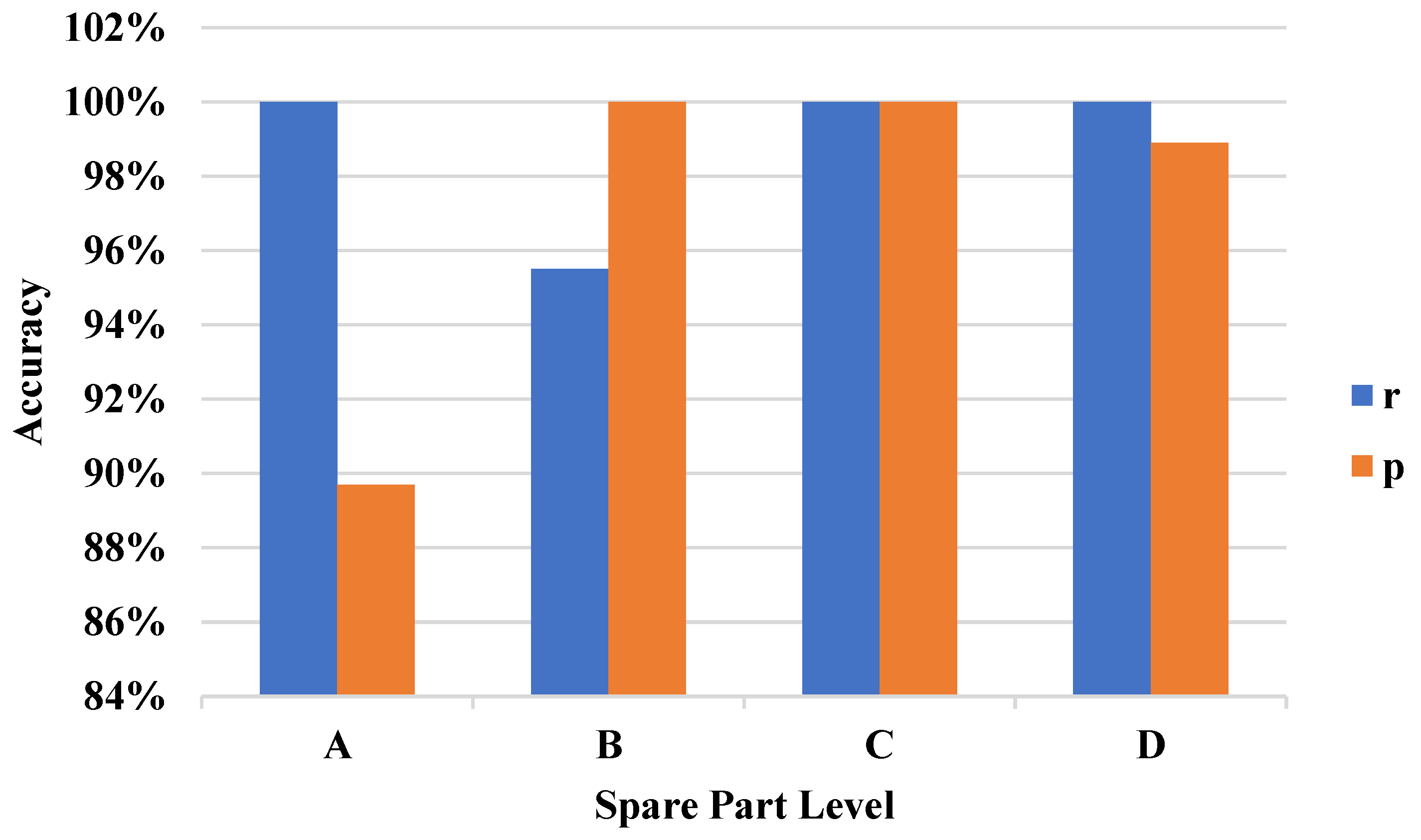
Figure 13 shows that with an increasing number of class A spare parts, the precision ratio increases to a very high level. Even without the final color box for the level judgment, the spare parts of different levels still have high
r and
p. Compared to supervised learning, the non-supervised learning shows lower precision for certain spare parts but the error is still within an acceptable range. The non-supervised results, in other words, do also demonstrate the effectiveness of the proposed method.
4.6. Comparative Study
We further compared the proposed method to other traditional classification methods including SVM, BP Neural Network (BPNN), and K-Nearest Neighbor (KNN) using the same dataset and accuracy indicator.
The SVM parameter with the cost coefficient and kernel function coefficient is 1 and
initially, where
is the number of the features. The BPNN has one input layer, one hidden layer, and one output layer. The numbers of input neurons, hidden neurons, and the output neurons are
,
, and
respectively, wherein
represents the number of the images and
is the characteristics of the image. There are 10 neighbors in the KNN.
Table 6 shows detailed information gathered in this comparative analysis, where the modified AlexNet structure shows the best average accuracy.
Table 9 shows that the average accuracy of the modified AlexNet structure for spare part classes A, B, C, and D is 0.90, 0.95, 1.0, and 0.99 respectively; the proposed method outperforms all other methods tested here in terms of average accuracy. The SVM algorithm produced relatively close results at 0.88, 0.90, 0.84, and 0.98 for classes A, B, C, and D, respectively. As discussed above, class A had the fewest samples while class C and D had more samples. However, the performance of the modified AlexNet structure is consistent for all four classes. This suggests that the proposed approach is effective regardless of the number of available datasets.
Neither SVM nor KNN is an effective tool for practical spare parts management because of their “black boxes”; they cannot offer understandable explanations to decision-makers regarding the rule’s assignment of criteria. The proposed method, conversely, makes the extracted criteria and hierarchical structure explicable and modifiable according to the expert knowledge or feedback based on the results. In the learning phase, the proposed method changes the traditional classification problem into an image classification problem which is helpful to the data visualization. It also outranks other methods tested here in terms of its accuracy and calculation speed.
5. Conclusions
For accurate spare parts classification, advanced condition monitoring technology should be developed and applied to the critical components, which will benefit a reliable maintenance logistics system. Moreover, this image identification method will also be considered to use for operation dashboard monitoring and fault diagnosis.
The graph-based deep convolutional neural network (G-DCNN) method developed in this study transforms the traditional classification problem into an image identification problem, realizing the visible and accurate classification of spare parts. The hierarchical classification structure is constructed to take unlimited criteria into consideration, which will be adjusted according to the practical demand. Additionally, the causal relationship between the criteria can be explained well through the hierarchical structure. Due to the transfer learning thought, AlexNet is modified to solve the spare parts classification problem by its excellent image identification ability. Both ReLu function and Dropout are adopted to eliminate overfitting problems under the condition of a two-GPU deep network. Through the case study results analysis, we can see a well performed model by cross validation and comparison. In particular, the influence of dataset amount to the learning model is obvious by A-class spare parts.
However, there are some problems unelaborated in this study that will be continued in the future. Regarding to the hierarchical structure, we intend to propose a quantitative approach that can deal with the causal relationship and status level division. With respect to the AlexNet application in spare parts classification, we may try to simplify its structure for more convenience in understanding and calculation in the future.


