Comparative Analysis of Exemplar-Based Approaches for Students’ Learning Style Diagnosis Purposes

Featured Application

Exemplar-based approach for students’ learning style diagnosis described in this paper may be applied in virtual learning environments; automatically predicted learning style may be used for personalizing virtual learning environments.

Abstract

A lot of computational models recently are undergoing rapid development. However, there is a conceptual and analytical gap in understanding the driving forces behind them. This paper focuses on the integration between computer science and social science (namely, education) for strengthening the visibility, recognition, and understanding the problems of simulation and modelling in social (educational) decision processes. The objective of the paper covers topics and streams on social-behavioural modelling and computational intelligence applications in education. To obtain the benefits of real, factual data for modeling student learning styles, this paper investigates exemplar-based approaches and possibilities to combine them with case-based reasoning methods for automatically predicting student learning styles in virtual learning environments. A comparative analysis of approaches combining exemplar-based modelling and case-based reasoning leads to the choice of the Bayesian Case model for diagnosing a student’s learning style based on the data about the student’s behavioral activities performed in an e-learning environment.

1. Introduction

This paper aims to present thorough, multidisciplinary research for making contributions, starting from concepts, models, and ending with recommendations and decision making capable to contribute to the effective educational policy formation agenda.

In modern educational theories, effective learning paths should take into account learners’ needs and characteristics [1]. According to [2], learners’ needs and characteristics are usually described in learners’ profiles (modules) and include prior knowledge, intellectual level, interests, goals, cognitive traits (working memory capacity, inductive reasoning ability, and associative learning skills), learning behavioural type (according to his/her self-regulation level), and, finally, learning styles.

Identification of students’ learning styles and creation of learning paths (scenarios) based on those learning styles using intelligent technologies has become a very popular topic in scientific literature [3,4]. Proper application of learning styles while creating optimal learning paths (scenarios) should result in higher student motivation, which in its turn is a good premise to improve learning results and effectiveness.

According to [5], a wide range of data about the behaviour of students in virtual learning environments should be used to generate good quality, real-time predictions about suitable materials and activities for each student individually. This should lead to success in acquiring knowledge and skills. In this case, a number of educational data mining and modelling methods and techniques could be used to identify and (if necessary) refine students’ learning styles.

In the current paper, the authors analyse an application of case-based reasoning (CBR) and Bayesian networks (BN) for students’ learning styles diagnosis. The objective of the research is to propose an exemplar-based probabilistic approach to model students’ learning style, as the current rule-based approaches or neural networks are mainly used for this purpose. In modelling, exemplar models explain real-life events that are problematic for modelling that uses sets of rules. Exemplar models are appropriate in situations where it is necessary to take into account the frequency effect, the dynamical aspects, and complexity. They use methods that generate models from data. Exemplar models aim to capture and store a detailed record of events over time and compare new observations against exemplars already stored. A new exemplar of the event is classified according to its similarity to the exemplars already stored. Similarity might be computed in various ways, such as the ‘distance’ between the new exemplar and the exemplar already stored in the parameter space, assessing similarity by conditional probability, i.e., computing the probability of the newly observed exemplar given the features of the exemplar or using any loss function. The best-known examples of exemplar-based modelling are the nearest neighbor method and case-based reasoning.

In this paper, first, a case-based reasoning (CBR) method that uses old experiences and adapts them for finding a solution to new problems is described. Then, graphical representation called Plate notation is briefly introduced. It is used to describe statistical models, including template models for graphical Bayesian network (BN) modelling. Second, a literature analysis on modelling approaches combining CBR and Bayes network is conducted, trying to identify the current status of the development of the framework for Bayesian case-based reasoning. The literature analysis focuses on exemplar-based approaches, exploring possibilities of combining BN and CBR and searching for niches to improve the overall BN + CBR approach. In the paper, a comparative analysis of existing CBR+BN models is conducted. Attention is paid to the learner’s feedback issues. Finally, after discussion and weighting the pros and cons of applying a combined BN-CBR approach for diagnosing student learning styles, conclusions are made and future research trends are presented, choosing the Bayesian case to model students’ learning style.

2. Methods

2.1. Combining Case-Based Reasoning and Bayesian Approach for Students’ Learning Style Modelling

As the aim of this scientific research is to explore possibilities and issues in the area of applying combined Bayesian and case-based reasoning approaches to model student learning styles, papers and video material on the theme were reviewed. A literature-based approach has been used. The target goal of the review of papers about Bayesian networks, mixture and mixed membership modelling (Latent Dirichlet allocation, topic models), case-based reasoning (CBR), rule-based reasoning (RBR) methods and their combination (Bayesian Case model (BCM) and interactive BCM (iBCM) [6], CBR + BN, CBR + RBR) was to comparatively analyze the main trends existing in the area of modelling, which integrates CBR methods for prediction, diagnosis, and reasoning. The potential to predict student learning styles based on his/her behavioral factors (learner’s behavioral activities in automated hypermedia learning systems) that determine learning style was discussed. As a result of the research, the Bayesian case model is proposed for dynamic prediction of a student’s learning style. BCM is a generative model, also known as “latent variable model”, which models uncertainty using probability and provides a way of modeling how a set of observed data arises from a set of underlying causes. As Bayesian probability theory is used for modelling aleatoric uncertainty, BCM combines a Bayesian approach with the case-based reasoning method, which models epistemic uncertainty arising due to limited knowledge or data. Using case-based reasoning, new problems are solved by retrieving cases describing similar prior problems from memory and adapting their solutions to the new case. In this way, BCM mimics the natural human decision-making process.

2.2. Case-Based Reasoning and Similarity-Based Retrieval

Following [7], case-based reasoning describes a methodology for solving problems. The term consists of case—an experience of a solved problem that may be represented in different ways; based—meaning that the reasoning is based on cases stored in case base; reasoning—meaning that conclusions should be made using cases, given a new problem to be solved. Major types of experiences occur in classification, diagnosis, prediction, planning, and configuration [7]. Using these experiences, solutions to new problems may be found and represented in different ways: commenting, presenting illustrations, explanations, advising, seeing that effects occurred in previous analogous situations, etc. In their content, these representations are some kinds of exemplars of previous experiences. Reasoning by exemplars imitates the natural process of human thinking [8]; therefore, it should be used in machine learning and artificial intelligence.

Applying case-based reasoning, we make an approximate reasoning using knowledge about previous experiences recorded as cases in a case base, which is also called memory. Knowledge can either be represented explicitly or be hidden (for example, in a latent variable, in an algorithm). The so-called “4R” process is performed in case-based reasoning: retrieve (search using index structure), reuse (adapt in various levels of granularity), revise (test in reality and modify), and retain (store/learn new case in case base in order to improve it) [7].

CBR divides an experience into two parts [7]: a problem part (description of a problem situation) and a solution part (description of the reaction to a situation). There are two major ways to formulate problems: standardized formulation (using mathematical models, formulas, etc.) and interactive formulation, using user’s feedback or dialogue with the user. In CBR, a failed solution is also an important piece of information and should be stored in the memory. Experiences may be saved in various forms: visual, textual, and conversational. In a typical, most simple way, cases are represented as feature–value pairs (also called attribute–value pairs) that need to be identified for both the problem and solution [7]. The concept of a feature’s importance (weight) also takes part. Authors of [7] describe the important attribute as one having a large influence on the choice of which case is the nearest neighbour. For case representation Case retrieval nets, the Dynamic Memory Model, and the Category and Exemplar Model may be used [9,10]. Cases may also be combined with other knowledge.

To reuse cases from the past, a recorded experience needs to be similar to the new problem. Thus, each attribute in a new case requires its own similarity function. In the similarity assessment, comparing new case with cases that already exist in the case base, the relative relevance of each attribute also has to be represented. The new case is most similar to the nearest neighbour’s case; therefore, the global similarity can be computed as sum of local similarities [7]:

$${\displaystyle \sum }_{\mathrm{i}=1}^{\mathrm{n}}\left({\mathrm{w}}_{\mathrm{i}}\ast \mathrm{sim}({\mathrm{x}}_{\mathrm{i}},{ \mathrm{y}}_{\mathrm{i}}\right))|1\le \mathrm{i}\le \mathrm{n}$$

(1)

Depending on a concrete task, similarity may be obtained in various ways: using the Euclidean distance, using a real-valued function, classification and clustering algorithms (fuzzy, nearest neighbour, etc.), and modelling similarity as the result of a dot product over feature vectors [11]. To compare a new case with past cases from the case base by using the common space of attributes, existing models for similarity-based retrieval may also be applied: ARCS, MAC/FAC models, etc. For example, [11] presents an efficient two-stage similarity-based model MAC/FAC, which uses content vectors to inexpensively search the memory first (MAC phase), and then applies a more expensive literal similarity matcher (FAC phase) for obtaining structurally sound matches.

After retrieval of the most similar case, an adaptation step may be performed in order to obtain the final solution to new problem.

2.3. Bayesian Approach and Bayesian Inference in Generative Models

The Bayesian approach to modeling uncertainty is useful when data are limited, worries about overfitting exist, there are reasons to believe that some facts are more likely than others, but that information is not contained in the data we model and when we are interested in precisely knowing how likely certain facts are, as opposed to just picking the most likely fact [12]. The core of Bayesian analysis is to marginalize over the posterior distribution of parameters so that a better prediction result is obtained, both in terms of accuracy and generalization capability [13].

For the problem of inferring parameter $\mathsf{\theta }$ for a distribution from a given set of data $\mathrm{x}$, Bayes’ theorem says that the posterior distribution is equal to the product of the likelihood function θ−>$\mathrm{p}(\mathrm{x}|\mathsf{\theta })$ and the prior $\mathrm{p}\left(\mathsf{\theta }\right)$, normalized by the probability of the data p(x) [14]:

$$\mathrm{p}\left(\mathsf{\theta },\mathrm{x}\right)=\frac{\mathrm{p}\left(\mathrm{x}|\mathsf{\theta }\right)\mathrm{p}\left(\mathsf{\theta }\right)}{{\displaystyle \int }(\mathrm{p}(\mathrm{x}|{\mathsf{\theta }}^{\prime })\mathrm{p}\left({\mathsf{\theta }}^{\prime }\right)|\mathrm{d}{\mathsf{\theta }}^{\prime })}$$

(2)

That means, to calculate the posterior we need to normalize by the integral. Since the likelihood function is usually defined from the data-generating process, we can see that the different prior choices can make the integral more or less difficult to calculate. If the prior has the same algebraic form as the likelihood, then we can obtain a closed-form expression for the posterior, avoiding the need for numerical integration [15]. This is the case of an analytical posterior distribution. For other cases, the standard Monte Carlo method can be used when we try to obtain a sampling approximation of the integral. In standard Monte Carlo integration, samples from a distribution are drawn, and some expectation is approximated using the sample average rather than calculating a difficult or intractable integral. In this case the Strong Law of Large Numbers is exploited [16].

In most cases it is hard to do exact inference in Bayesian networks, even in simple cases, as the posterior distribution is not analytically solvable [17]. Only few cases exist when exact inference is possible [17]: in large models, when latent variables are not cyclic; when the prior and posterior are conjugate distributions, having conjugate prior to the likelihood function; and when distributions have finite support, as a discrete distribution with finite support can only have a finite number of possible realizations [17].

An approximate inference quite often includes parts of exact inference [17]. In making an approximate inference using the Bayesian approach, few cases can also be distinguished [17]:

• using Monte Carlo methods (for example, Gibbs sampling), when posterior distribution is represented as a collection of weighted samples;
• representing posterior distribution as parametric distribution and using variational methods for analytical approximation to the posterior probability of the unobserved variables;
• making amortized inference: learning to do inference quickly (“bottom-up”, “pattern-recognition”, “data-driven”).

The idea of the Monte Carlo method is to use some agent (for example, Gibbs sampler) to sample from the prior distribution and weight by likelihood (or transform samples so that they become samples from the posterior) [17]. As simply “guessing” from a prior distribution makes sampling inefficient, there are types of sampling that use some guiding distribution. For example, in importance sampling, sampling is done from guide $\mathrm{q}\left(\mathrm{z}\right)$, weighting by $\mathrm{w}=\frac{\mathrm{p}\left(\mathrm{z},\mathrm{x}\right)}{\mathrm{q}\left(\mathrm{z}\right)}$. It is like “a good guess”, when guiding distribution is considered to be close to the real posterior distribution, parameters of which we compute. When needed, a guiding distribution also may be learned from the neural network [17]. In the Markov chain Monte Carlo (MCMC) method, when conditional distributions are not known exactly, a “guide” is proposed, and the proposal is accepted or rejected using feedback from model [17]. In other words, instead of using a predetermined guide distribution, as this is done in the case of importance sampling, random walking over $\mathrm{Z}$ is performed. $\mathrm{Z}$ is such that the proportion of samples ${\mathrm{z}}^{\ast }$ is proportional to $\mathrm{p}\left({\mathrm{z}}^{\ast }|\mathrm{x}\right)$. Randomly walking, we take correlated samples from a Markov chain, and a new sample is based on the feedback from the previous sample. In MCMC it is presumed that the posterior distribution is stationary [17].

Having a prior distribution of latent variables, generative models predict the likelihood of observations (poster distribution), given a latent variable. The Monte Carlo approach is used to generate a hypothetical posterior distribution based on “guess parameters”. Having a prior over the parameters and some likelihood function, it is possible to combine those to compute the posterior of the parameters (according to Bayes theorem):

$$\mathrm{p}\left(\mathsf{\theta }|\mathrm{X}\right)=\frac{\mathrm{p}\left(\mathrm{X}|\mathsf{\theta }\right)\mathrm{p}\left(\mathsf{\theta }\right)}{\mathrm{p}\left(\mathrm{X}\right)}$$

(3)

Here, $\mathrm{p}\left(\mathsf{\theta }|\mathrm{X}\right)$ is the posterior, $\mathrm{p}\left(\mathrm{X}|\mathsf{\theta }\right)$ is likelihood, $\mathrm{p}\left(\mathsf{\theta }\right)$ is prior, and $\mathrm{p}\left(\mathrm{X}\right)$ is a normalizing constant.

MCMC is applied when direct sampling from joint posterior distribution is difficult. It uses Gibbs sampling to estimate the model parameters, i.e., evaluation of the conditional posterior distribution of each variable conditioned on the other variables. In other words, Gibbs sampling is used to obtain a sample from the posterior distribution with multiple variables. In Gibbs sampling the conditional probability of one axis given all the others must be computed, i.e., sampling from all of the conditional distributions for all the model’s parameters must be possible. Practical difficulty is faced in that this is rarely possible unless only simple models are used. In Gibbs sampling the parameter value simulated from its posterior distribution in one iteration step is used as the conditional value in the next step [18]. Repeating the process provides the result of an approximate random sample to be drawn from the posterior distribution. Sampling begins by creating a preliminary clustering to generate start values for the parameters [18]. The start values may be determined through a qualified guess or using neutral values. Clustering is preferred since the Markov chains converge faster when the start values are closer to their target values. A non-hierarchical clustering is used with an iterative algorithm that minimizes the sum of distances from each object to its cluster centroid, over all clusters. This algorithm moves objects between clusters until the sum cannot be decreased further. The result is a set of clusters that are compact and well-separated [18]. As Gibbs sampling is slow, collapsed Gibbs sampling is used. Its idea is to sample from a distribution with one of the conditioned variables (one of the full conditionals) integrated out.

Thus, in summary, in Bayesian updating without a prior conjugate, the Gibbs update on a randomly chosen subset of the new full data set is performed since previous data points are dependent on the new data (for example, Latent Dirichlet allocation (LDA) uses Gibbs sampling algorithm [19]). The size of the subset may be adjusted to achieve an appropriate trade-off between speed and accuracy [16]. Theoretically, the data are generated by the following process: first, $\mathrm{p}\left(\mathsf{\theta }\right)$ is sampled, and then the observables x from a distribution which depends on θ are sampled, i.e., $\mathrm{p}\left(\mathsf{\theta },\mathrm{X}\right)=\mathrm{p}\left(\mathsf{\theta }\right)\times \mathrm{p}(\mathrm{x}|\mathsf{\theta })$. Note that $\mathrm{p}(\mathrm{x}|\mathsf{\theta })$ can take a variety of parametric forms [20].

For classical Bayesian inference, assumption about a likelihood function for the data must be done, and then parameters may be estimated. However, here every sample from the posterior is some setting of “guess parameters”. Posterior means can be computed to get a single “best” value of parameters (averaging the samples). The “best” in that case would be in the sense of minimizing the expected squared distance from the true parameters [21]. In Gibbs sampling, samples are simulated from a generative process. All conditional distributions of the target distribution are sampled exactly. When drawing from the full-conditional distributions is not straightforward (not having obtained the full conditional distribution), other samplers “within-Gibbs” are used, for example, Metropolis hasting rejection sampling for Markov chains.

2.4. Related Works

General knowledge may be modeled by statistical distributions [22]. The type of uncertainty that deals with assigning a probability of a particular state given a known distribution is referred to as aleatory uncertainty, which can perfectly be modelled using Bayesian networks. In Bayesian reasoning, uncertainty about the unknown parameter is represented by a probability distribution. This probability distribution is subjective and reflects personal judgment of uncertainty. Another type of uncertainty, epistemic uncertainty, is related to cognitive mechanisms of knowledge processing; therefore, some lack of knowledge exists in a sense that it is limited by knowledge processing mechanisms. Epistemic uncertainty is also known as systematic uncertainty, which is due to things one could in principle know but does not know in practice. The case-based reasoning method is applied for modelling epistemic uncertainty. It is based on situation-specific experiences and episodic knowledge [23].

For better decision making that includes both types of uncertainty, it may be appropriate to apply a combination of the CBR method and Bayesian network model. Therefore, literature on combining CBR with BN has been reviewed.

Authors in [22] state that CBR and BN can be combined in parallel, in sequence BN -> CBR, and in sequence CBR -> BN.

According to [23], in Artificial Intelligence, integration or a combination of various methods is a popular approach. Authors of [23] introduce the basic types of case-based reasoning integrations and indicate that case-based reasoning is usually combined with rule-based reasoning [24], model-based reasoning, and soft computing methods (i.e., fuzzy methods, neural networks, genetic algorithms). They distinguish five combinations of models depending on the degree of coupling between integrated components: standalone, transformational, loose coupling, tight coupling, and fully integrated. Authors of [23] also systematize intelligent methods for CBR integration. According to their research results, most of the efforts to integrate CBR with other methods or models have been input into CBR integration with rule-based reasoning systems.

Authors in [25] present different architectures for CBR and BN combinations. In a parallel way, both methods use all of the input variables and then produce a classification independently. Authors in [25] introduce metareasoner, which decides during runtime which strategy to use (based on Bayesian network or on CBR) according to collected performance data. It is assumed that a method or model that performed well on a previous task will continue to do so in the future as learning is gradual.

Authors in [26] describe a technique that integrates CBR and BN to build user profiles incrementally. Regardless of the diversity of various architectures, the main way of integrating CBR and BN is through a common space between CBR and BN parameters (a generalizing schema is presented by [27]), comparing new observations with all retrieved cases and trying to find the most similar ones.

Authors in [28] conducted trials to combine CBR and semantic networks. The goal was to generate more detailed and meaningful explanations. Authors mentioned that, in this case, a challenge is the lack of a formal basis for the semantic network.

Qualitative comparison between CBR and BN is made by [29]. It is stated that difficulties in BN are computational complexity, in the case of big data sets, and difficulty to obtain the initial parameters or add a new node. CBR is treated as an easier approach that has the main difficulty of describing cases by experts.

Authors in [30] describe an optimized hybrid approach for fault diagnosis using a combination of BN and CBR. The Chi-square test is applied instead of heuristic algorithms for construction of BN and modification of its structure in the case of newly added nodes or removed ones. Optimization for message passing is also proposed: when a problem occurs, instead of the usual inference performed on all the nodes of BN, the inference process is executed only on a subset of nodes. This shortens computational time.

In [31] a combination of BN (dynamic part) and semantic network (static part) for domain modelling is presented, and Bayesian case retrieval as a two-step process is described.

Not one single author (for example [32,33]) emphasized a lack of experimental work in the field of automatic learner’s model generation and personalization of learning environments.

2.5. Modelling Based on Bayesian Approach and/or Case-Based Reasoning

2.5.1. Mixture Model

Mixture models are flexible tools that allow modelling the associated structure of a set of variables (their joint density) using a finite mixture of simpler densities [34]. Mixture models have a single latent variable (called indicator variable) that points to the mixture component. Mixture components can be modeled using a prior distribution for mixing proportions that selects a reasonable subset of components to explain any finite training set [35]. Formally, the mixture model is defined in the following way:

$$\mathrm{P}\left(\mathrm{x}\right)={\displaystyle \prod }_{\mathrm{i}=1}^{\mathrm{n}}{\displaystyle \sum }_{{\mathrm{c}}_{\mathrm{i}}=1}^{\mathrm{K}}\left(\mathrm{p}({\mathrm{c}}_{\mathrm{i}}\right)\mathrm{p}({\mathrm{x}}_{\mathrm{i}}|{\mathrm{c}}_{\mathrm{i}})); \mathrm{X}=\{{\mathrm{x}}_{\mathrm{i}}, \dots ,{\mathrm{x}}_{\mathrm{n}}\};$$

(4)

Here,$\mathrm{p}\left({\mathrm{c}}_{\mathrm{i}}\right)$ is the probability that the example is in cluster ${\mathrm{c}}_{\mathrm{i}}$. $\mathrm{p}({\mathrm{x}}_{\mathrm{i}}|{\mathrm{c}}_{\mathrm{i}})$ is the probability of ${\mathrm{x}}_{\mathrm{i}}$ if i is in cluster ${\mathrm{c}}_{\mathrm{i}}$ The generative process of the mixture model consists of cluster sampling and sampling data examples from the cluster distribution. Mixture models infer mixtures of distributions for each component separately. In most cases, the goal to compute posterior distributions of parameters or latent variables requires multidimensional integration. Deriving posterior means or simply identifying regions of high posterior density value pose highly complex computational challenges. Standard Monte Carlo methods are available for simulating from a posterior distribution associated with a mixture [36], allowing implicit integration over the entire parameter space.

By the law of large numbers, integrals described by the expected value of some random variable can be approximated by taking the empirical mean (the sample mean) of independent samples of the variable. When the probability distribution of the variable is parametrized, Markov chain Monte Carlo (MCMC) sampler may be used [13]. As to draw independent samples from a joint posterior distribution is computationally intractable, a Markov chain is constructed, i.e., MCMC generates samples from the posterior distribution by constructing a reversible Markov chain [37]. It is expected that in a very long run samples will take values that look like draws from the target distribution (at equilibrium). By the ergodic theorem, the stationary distribution is approximated by the empirical measures of the random states of the MCMC sampler [13]. Various algorithms are used for posterior sampling (i.e., sampling to generate the posterior distribution); for high-dimensional Gaussian distributions, Gibbs sampler is recommended [36], which is used to approximate the hidden variable distributions. These determine the next steps of the Markov chain.

2.5.2. Latent Dirichlet Allocation-Mixed Membership Model

As the research includes Bayesian methods that may be used for students’ learning style modelling, first, we briefly describe Latent Dirichlet allocation, which is a generative model for collections of discrete data, a sophisticated application of the Bayesian technique. As typically LDA is used in topic models to classify text in a document to a particular topic, LDA is described using a topic modelling example. Then, it is adapted to learning style modelling by analogy. Section 2.5.3 and Section 2.6.1 explain how the LDA approach may be used to model learning style.

In topic modelling, documents are represented as random mixtures over latent topics, where each topic is characterized by a distribution over all the words. LDA builds a topic per document model and words per topic model, modeled as Dirichlet distributions. Each document is modeled as a multinomial distribution of topics, and each topic is modeled as a multinomial distribution of words. LDA assumes that documents are produced from a mixture of topics. Preprocessing of the raw text, conversion of text to a bag of words, and specification of how many topics are in the data set are made before LDA is performed [38]. As [15] explains, LDA works by first making a key assumption: the way a document was generated was by picking a set of topics and then for each topic picking a set of words. So, LDA reverse-engineers this process. LDA assumes that the prior is arising from the Dirichlet distribution. At each iteration, the posterior is updated in order to reflect more proper topics. To find groups of tightly co-occurring words, LDA has a trade-off two goals: for each document, allocate its words to as few topics as possible, and for each topic, assign high probability to as few terms as possible [39]. In LDA, it is a must to specify the number of topics first. Thus, we have the probability distribution of topics in documents, which indicates how much the document “likes” the topic, and the probability distribution of words in topics indicates how much a topic “likes” a word.

Following [40], in LDA, we assume that words are generated by topics (by fixed conditional distributions) and that those topics are infinitely exchangeable within the document. An infinite sequence of random variables is infinitely exchangeable if every finite subsequence is exchangeable. De Finetti’s representation theorem states that exchangeable observations are conditionally independent relative to some latent variable, and an epistemic probability distribution could then be assigned to this variable. Authors of [40] refine that the joint distribution of an infinitely exchangeable sequence of random variables is as if a random parameter was drawn from some distribution; then the random variables in question were independent and identically distributed, conditioned on that parameter. By de Finetti’s theorem, the probability of a sequence of words and topics must therefore have the form:

$$\mathrm{p}\left(\mathrm{w},\mathrm{z}\right)={\displaystyle \int }\mathrm{p}\left(\mathsf{\theta }\right){\displaystyle \prod }\mathrm{p}({\mathrm{z}}_{\mathrm{n}}|\mathsf{\theta })\mathrm{p}\left({\mathrm{w}}_{\mathrm{n}}{|\mathrm{z}}_{\mathrm{n}}\right)\mathrm{d}\mathsf{\theta }$$

(5)

$\mathsf{\theta }$ is the random parameter of a multinomial distribution over topics, and w is a document in the document corpus. The text of a document is treated as bag of words disregarding grammar and even word order but keeping multiplicity. $\mathrm{z}$ is a hidden topic variable. LDA distribution on documents is obtained by marginalizing out the topic variables and endowing $\mathsf{\theta }$ with a Dirichlet distribution [40].

Using LDA for making inference, it is needed to compute the posterior distribution of the hidden variables given a document:

$$\mathrm{p}\left(\mathsf{\theta },\mathrm{z}|\mathrm{w},\mathsf{\alpha },\mathsf{\beta }\right)=\frac{\mathrm{p}\left(\mathsf{\theta },\mathrm{z},\mathrm{w}|\mathsf{\alpha },\mathsf{\beta }\right)}{\mathrm{p}(\mathrm{w}|\mathsf{\alpha },\mathsf{\beta })}$$

(6)

Parameters $\mathsf{\alpha }$ and $\mathsf{\beta }$ are corpus-level parameters, assumed to be sampled once in the process of generating a corpus. Although the posterior distribution is intractable for exact inference, a wide variety of approximate inference algorithms can be considered for LDA, including Laplace approximation, variational approximation, and Markov chain Monte Carlo [40]. Applying MCMC, all latent variables are sampled from the posterior distribution. Gibbs sampling may be used. In addition to variational methods, it is also worth to mention the possibility to use Non-negative Matrix Factorization with Kullback Leibler divergence (NMF-KL), which approximates the LDA model under a uniform Dirichlet distribution. In the context of comparing the multiplicative algorithm to solve NMF-KL with the variational inference algorithm for LDA, it can be stated that the NMF-KL “multiplicative updates roles” can be approximated to the updates established by variational inference algorithm for LDA [41].

2.5.3. Differences between Mixed and Mixed Membership Models

There is a difference between pure Mixture model and model, using Latent Dirichlet allocation (LDA) (called “mixed membership model”). Mixed-membership model is an extension of the mixture model to grouped data where each “data point” is itself a collection of data, and each collection can belong to multiple groups. Mixed membership model captures both homogeneity and heterogeneity, but a mixture is less heterogeneous, as each group can only exhibit one component. In contrast to mixture models, mixed membership models (also referred to as partial membership models) assume that observational data points may only partly belong to population mixture categories, referred to in various fields as topics, extreme profiles, pure or ideal types, states, or subpopulations (for students’ learning style modelling-learning styles). The degree of membership then is a vector of continuous non-negative latent variables that adds up to 1 [42]. For example, documents each may exhibit multiple themes and to different degrees. Mixed membership models share the same set of distributions on words, but mix over them differently for each group. In turn, in mixture models, membership is a binary indicator [42]. Mixture models are a way of putting similar data points together into “clusters”, where clusters are represented by the component distributions. The idea is that all data points of the same type, belonging to the same cluster, are more or less equivalent and all come from the same distribution, and any differences between them are matters of chance [43].

In a mixture model, for students’ learning style modelling, behavioral activities in a student’s log are presumed to co-occur, and, given that, the entire student’s log is assigned a single learning style cluster (inference about the highest probable learning style of the learner is made); in turn, in a mixed-membership model, it is presumed that behavioral activities co-occur in a learning style cluster within a student’s log, and the model returns the highest probable clusters in that log (i.e., each log has a distribution over the prevalence of learning styles in that log) [15].

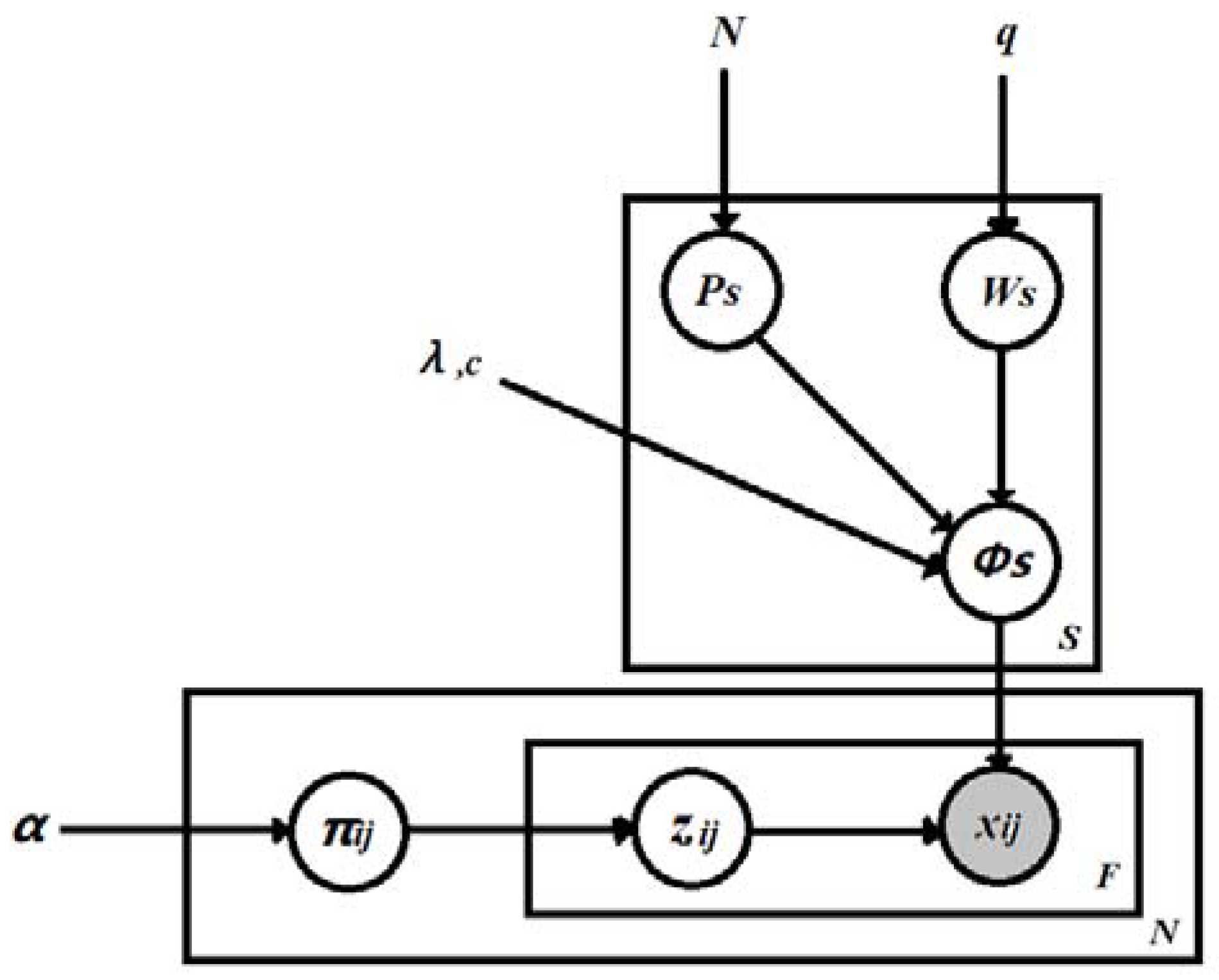
2.5.4. Bayesian Case Model

Bayesian case model is comprehensively presented by Been Kim and her colleagues [8]. Been Kim states that BCM is a general framework for Bayesian case-based reasoning (CBR) and prototype classification and clustering. It brings the intuitive power of CBR to a Bayesian generative framework, performing joint inference on clustering and explanations of the clusters. BCM captures dependencies among features via prototypes [8].

BCM is a discrete mixture model, i.e., it treats data as a mixture of several components. Each feature belongs to one of the components, and each component has a simple parametric form [8]. BCM is a generative statistical model that has clustering and explanation parts [8]. Thus, having N observations ($\mathrm{X}=\{{\mathrm{x}}_{\mathrm{i}}, \dots ,{\mathrm{x}}_{\mathrm{n}}\}$), each ${\mathrm{x}}_{\mathrm{i}}$ represents a random mixture over clusters. Generative models can specify a joint probability distribution over observed variables and latent variables, i.e., given an observable variable $\mathrm{X}$ and a target variable $\mathrm{Y}$, it models the joint probability distribution on $\mathrm{X}\times \mathrm{Y}$. That is, a generative model is a model of the conditional probability of the observable $\mathrm{X}$, given a target Y:p($\mathrm{X}$|$\mathrm{Y}$ = x).

BCM generates each observation using the important pieces of related prototypes [8]. As in BCM, the underlying structure of the observations is represented by a standard discrete mixture model, each feature $\mathrm{j}$ of the observation $\mathrm{i}({\mathrm{x}}_{\mathrm{i}}$) comes from one of the clusters, the index of the cluster for ${\mathrm{x}}_{\mathrm{ij}}$ is denoted by ${\mathrm{z}}_{\mathrm{ij}}$, and the full set of cluster assignments for observation–feature pairs is denoted by $\mathrm{z}$. Each ${\mathrm{z}}_{\mathrm{ij}}$ takes on the value of a cluster index between 1 and $\mathrm{S}$ [8]. BCM augments the standard mixture model with prototypes and subspace feature indicators that characterize the clusters, thus making BCM more interpretable. BCM allows sets of observations to be explained by latent variable $\mathrm{z}$, i.e., to infer why some parts of the data are similar. In mixture models, the latent variable $\mathrm{z}$ corresponds to the mixture component, and it takes values in a discrete set; thus, $\mathrm{p}\left(\mathrm{z}\right)$ is always a multinomial distribution. A graphical representation of BCM is presented in Figure 1 [8]. The model is presented in Plate notation [44,45].

Authors in [8] also presented the full BCM model in statistical form:

• ${\mathsf{\varphi }}_{\mathrm{sj}}~\mathrm{Dirichlet}({\mathrm{g}}_{{\mathrm{p}}_{\mathrm{sj}},{\mathrm{w}}_{\mathrm{sj}\mathsf{\lambda }}})$ ∀ s, j;
• ${\mathrm{g}}_{{\mathrm{p}}_{\mathrm{sj}},{\mathrm{w}}_{\mathrm{sj}\mathsf{\lambda },}}\left(\mathrm{v}\right)=\mathsf{\lambda }(1+\mathrm{c}{1}_{\left[{\mathrm{w}}_{\mathrm{sj}}=1{ \mathrm{and} \mathrm{p}}_{\mathrm{sj}}=\mathsf{\theta }\right]})$;
• ${\mathrm{p}}_{\mathrm{s}}~\mathrm{Uniform} \left(1, \mathrm{N}\right)\forall \mathrm{s};$
• ${\mathrm{w}}_{\mathrm{sj}}~\mathrm{Bernoulli}\left(\mathrm{q}\right)\forall \mathrm{s}, \mathrm{j};$
• ${\mathsf{\pi }}_{\mathrm{i}}~\mathrm{Dirichlet}\left(\mathsf{\alpha }\right)\forall \mathrm{i};$
• ${\mathrm{z}}_{\mathrm{ij}}$~Multinomial (${\mathsf{\pi }}_{\mathrm{i}}$) ∀ i, j;
• ${\mathrm{x}}_{\mathrm{ij}}$~Multinomial (${\mathsf{\varphi }}_{{\mathrm{z}}_{\mathrm{ij}}}$) ∀ i, j;

As it is presented in the model, there are some hyperparameters $\left(\mathrm{c}, \mathsf{\lambda }, \mathrm{q}\right)$ in BCM. Generally, parameters can help in defining or classifying a particular system. Parameters of the priori are called hyperparameters. It is a typical characteristic of conjugate priors that the dimensionality of the hyperparameters is one greater than that of the parameters of the original distribution. In the mixture model, using the Bayesian setting, the mixture weights and parameters themselves are random variables, and prior distributions will be placed over the variables. In BCM, the weights are typically viewed as a K-dimensional random vector drawn from a Dirichlet distribution (i.e., from the conjugate prior of the categorical distribution), and the parameters are distributed according to their respective conjugate priors.

Authors in [8] emphasize that in BCM c and $\mathsf{\lambda }$ are constant hyperparameters that indicate how much the prototype will be copied in order to generate the observations. Setting $\mathrm{c}, \mathsf{\lambda },$ and $\mathrm{q}$ can be done through cross-validation, another layer of hierarchy with more diffuse hyperparameters, or plain intuition. For $\mathsf{\alpha }$ there are natural settings (all entries being 1) [8]. Mixture weights ${\mathsf{\pi }}_{\mathrm{i}}$ (proportion of elements in each cluster) are generated according to a Dirichlet distribution, parameterized by hyperparameter $\mathsf{\alpha }$. Hyperparameter $\mathsf{\alpha }$ “controls” how many different clusters we want to have per data point, i.e., per log of the student. To use BCM for classification, vector ${\mathsf{\pi }}_{\mathrm{i}}$ is used as $\mathrm{S}$ features for a classifier, such as SVM [8], which categorizes unlabeled data, representing the examples as points in space, mapped so that the examples of the separate categories are divided by a clear gap that is as wide as possible. New examples are then mapped into that same space and predicted to belong to a category based on which side of the gap they fall [8]. It must be noted that Dirichlet is the prior conjugate for categorical (multinomial) distribution; therefore, sampling is not necessary in this case, as it is possible to marginalize and evaluate the probability distribution exactly.

The generative model is trained with a large amount of data; after training, it is able to generate data similar to the initial set of data. There are some methods developed for pre-training for generative modelling: Maximum Likelihood Estimation, variance algorithms, Markov Monte Carlo method, and others [46]. As it has already been mentioned, generally, generation can be done by sampling from prior and weighting by likelihood (it is the expectation maximization method), using some guide distribution (it is called importance sampling), using Markov Monte Carlo (iteratively sampling the unknown variables of the model from their conditional distributions), or variational methods. Markov chain sampling methods for Dirichlet process mixture models are presented in [47].

In the BCM generative story, clusters are generated first (each data point is repesented by distribution over clusters). Prototype ${\mathrm{p}}_{\mathrm{s}}$ is generated by sampling uniformly over all observations [8], i.e., initially it is presumed that every cluster is equally probable. Each element of the feature indicator vector ${\mathrm{w}}_{\mathrm{sj}}$ that indicates important features for the cluster is generated according to a Bernoulli distribution with hyperparameter $\mathrm{q}$ [8]. The distribution of feature outcomes ${\mathsf{\varphi }}_{\mathrm{s}}$ for cluster s is generated so that it mostly takes outcomes from the prototype ${\mathrm{p}}_{\mathrm{s}}$ for the important dimensions of the cluster. It is determined by vector g indexed by possible outcomes v through ${\mathsf{\varphi }}_{\mathrm{sj}}~\mathrm{Dirichlet}({\mathrm{g}}_{{\mathrm{p}}_{\mathrm{sj}},{\mathrm{w}}_{\mathrm{sj}\mathsf{\lambda },}})$:

$${\mathrm{g}}_{{\mathrm{p}}_{\mathrm{sj}},{\mathrm{w}}_{\mathrm{sj}\mathsf{\lambda },}}\left(\mathrm{v}\right)=\mathsf{\lambda }(1+\mathrm{c}{1}_{\left[{\mathrm{w}}_{\mathrm{sj}}=1{ \mathrm{and} \mathrm{p}}_{\mathrm{sj}}=\mathsf{\theta }\right]})$$

(7)

Here, $\mathrm{c}$ and $\mathsf{\lambda }$ are constant hyperparameters that indicate how much we will copy the prototype in order to generate the observations [8].

Authors in [8] clarify that the explanatory power of BCM results from how the clusters are characterized. While a standard mixture model assumes that each cluster takes the form of a predefined parametric distribution, BCM characterizes each cluster by a prototype ${\mathrm{p}}_{\mathrm{s}}$ and a subspace feature indicator ${\mathrm{w}}_{\mathrm{sj}}$. Intuitively, the subspace feature indicator selects only a few features that play an important role in identifying the cluster and prototype.

BCM performs joint inference on latent variables: cluster labels ${\mathrm{z}}_{\mathrm{ij}}$, prototypes ${\mathrm{p}}_{\mathrm{s}}$, and important features ${\mathrm{w}}_{\mathrm{sj}}$. $\mathsf{\varphi }$ and $\mathsf{\pi }$ are integrated out. Collapsed Gibbs sampling is applied to perform inference, as this has been observed to converge quickly, particularly in mixture models [8].

2.6. Proposed Approach for Students’ Learning Style Prediction

2.6.1. Bayesian Case Model for Students’ Learning Style Modelling

When applying the Bayesian approach for student’s learning style identification, learning style is considered as latent parameter of interest $\mathsf{\theta }$, and student’s log consisting of his/her behavioral activities is considered as an observation ${\mathrm{x}}_{\mathrm{i}}$. $\mathrm{X}=\{{\mathrm{x}}_{\mathrm{i}}, \dots ,{\mathrm{x}}_{\mathrm{n}}\}$ will be a set of complete observations from a density that depends on $\mathsf{\theta }:\mathsf{\pi }(\mathrm{x}|\mathsf{\theta })$. According to the Bayes theorem, inference on the conditional probability of student’s learning style is based on posterior distribution of θ, using a prior distribution $\mathsf{\pi }\left(\mathsf{\theta }\right):$

$$\mathsf{\pi }\left(\mathsf{\theta }|\mathrm{X}\right)={\displaystyle \prod }_{\mathrm{i}=1}^{\mathrm{n}}\frac{\mathsf{\pi }\left({\mathrm{x}}_{\mathrm{i}}|\mathsf{\theta }\right)\mathsf{\pi }\left(\mathsf{\theta }\right)}{\mathsf{\pi }\left(\mathrm{X}\right)}$$

(8)

Here, $\mathsf{\pi }\left(\mathrm{X}\right)={\displaystyle \int }{\displaystyle \prod }_{\mathrm{i}=1}^{\mathrm{n}}(\mathsf{\pi }\left({\mathrm{x}}_{\mathrm{i}}|\mathsf{\theta })\mathsf{\pi }\left(\mathsf{\theta }\right)\mathrm{d}\mathsf{\theta }\right)$ is the marginal density of $\mathrm{X}$. For future observation ${\mathrm{x}}_{\mathrm{n}+1}$, its predictive distribution after observing ${\mathrm{x}}_1$, ${\mathrm{x}}_2$, …, ${\mathrm{x}}_{\mathrm{n}}$ can be computed as

$$\mathsf{\pi }\left({\mathrm{x}}_{\mathrm{n}+1}|\mathrm{X}\right)={\displaystyle \int }\mathsf{\pi }({\mathrm{x}}_{\mathrm{n}+1}|\mathsf{\theta }){\displaystyle \prod }_{\mathrm{i}=1}^{\mathrm{n}}\frac{\mathsf{\pi }\left({\mathrm{x}}_{\mathrm{i}}|\mathsf{\theta }\right)\mathsf{\pi }\left(\mathsf{\theta }\right)}{\mathsf{\pi }\left(\mathrm{X}\right)\mathrm{d}\mathsf{\theta }}=\mathsf{\pi }\left(\left\{\mathrm{X},{\mathrm{x}}_{\mathrm{n}+1}\right\})/\mathsf{\pi }(\mathrm{X}\right)$$

(9)

As it has already been mentioned in this paper, for approximate inference Gibbs sampling may be performed. For the sake of context, we briefly recall that Gibbs sampler is a Markov chain Monte Carlo algorithm for obtaining a sequence of observations that are approximated from a specified multivariate probability distribution, when direct sampling is difficult [48]. In Markov chain Monte Carlo, especially in Gibbs sampling, a collapsing down procedure for reducing random components may be used [49]. The idea of collapsing means skipping the steps of sampling parameter(s) values in standard data augmentation [49]. One or some parameters (called nuisance parameters) may be eliminated by integrating them out, i.e., marginalizing (focusing on the sums of distributions in the margin) over the distribution of the variables being discarded. Gibbs sampler, which integrates out (marginalizes over) one or more variables when sampling for some other variable, is called collapsed Gibbs sampler.

Model-based student learning style clustering is based on a finite mixture of distributions, in which each mixture component is taken to correspond to a different learning style cluster. The LDA framework models a per-cluster distribution of behavioral activities of the student, helping to understand what cluster each activity might be referring to. LDA treats each learning style cluster assignment as a multinomial random variable drawn from a symmetric Dirichlet and logistic normal prior. Inference algorithms build the latent space, a collection of learning styles for the corpus and a collection of learning style proportions for each of its logs. Mixed membership models allow each student’s log to exhibit multiple components, where each component is a distribution over behavioral activities. Conditioned on collection, inspecting the posterior of the components reveals the “learning styles” inherent in the logs, i.e., the significant patterns of activities associated under a single learning style [42].

In the case of exemplar-based dynamic modeling of students’ learning style using BCM, the model could generate student learning style clusters based on historical data about the student’s behavioral activities in a virtual learning environment. A principal diagram depicting BCM application for modelling students’ learning style using students’ behavioral data in virtual learning environment is presented in Figure 2. First, data mining of students’ logs stored in a virtual learning environment (VLE) must be done. The result of the data mining procedure should be a set of logs each consisting of a particular student’s behavioral activities in a virtual learning environment. Each log should be presented as bag of independent data objects, i.e., student’s behavioral activities that reflect his/her learning style (data objects are correlated in some way, representing the student’s learning style). Data mining methods were explored and described by authors in [50], but this paper focuses on BN + CBR modelling only.

In students’ leaning style model, which is a model of high-dimensional discrete data, we model student behavioral activity data in a virtual learning environment as coming from a mixture distribution, with mixture components corresponding to learning style clusters. We use the following notions. Observation is log with student’s behavioral activities stored. Having groups of observations, each group is modeled with a mixture. Components are distributions over the vocabulary of behavioral activities (recurring patterns of observed activities). The posterior components look like learning styles (distributions that place their mass on behavioral activities that exhibit a learning style). Probabilities associated with each component are called the mixture weights. The mixture components (the individual distributions that are combined to form the mixture distribution) are shared across groups. Proportions are how much each log reflects each learning style pattern. The mixture proportions vary from group to group. For example, a log that is half of one learning style and half of another learning style will place the corresponding proportions in those two learning styles.

Thus, BCM treats each log as a mixture of leaning styles. Proportions of learning styles are drawn once per document, and learning styles are shared across the corpus. In other words, BCM predicts student’s learning style, presenting it in the form of proportions of learning style clusters. Each cluster is represented by the prototype and important features. As BCM is an exemplar-based model, prototypes and important features representing each cluster are the real students’ behavioral activities performed in the virtual learning environment.

To the best of our knowledge, BCM has never been applied for modelling learning style in adaptive hypermedia learning systems. Thus, application of the exemplar-based Bayesian case model that uses a combined CBR + BN approach for student’s learning style modelling is new. The key difference between BCM and other approaches proposed for student learning style modelling is that BCM captures learning style “patterns” as real data examples rather than uses a classification of learning styles described in advance by experts. BCM’s ability to describe each learning style cluster by the prototype and subspace feature indicators may be considered as an advantage that contributes to a better understanding of generated learning styles.

2.6.2. Enhanced Bayesian Case Model: Interactivity

Authors in [6] also present an iBCM-interactive Bayesian case model, which is able to use feedback from a user and integrate knowledge transferred interactively into the model. This capability is beneficial to learning style modelling in that each student is presented a possibility to specify his/her preferences, i.e., what features are most important for him/her or which actual log should be considered as prototype. Following [6], users provide direct input to iBCM in order to achieve effective clustering results, and iBCM optimizes the clustering by achieving a balance between what the actual data indicate and what the user indicates as useful. iBCM lets users interact directly with a representation that maps parameters of the model. Besides that, iBCM explains its internal states in an easy-to-understand manner. For implementation of interactivity, iBCM introduces interacted latent variables that represent a variable inferred through both user feedback and the data [6].

2.6.3. Bayesian Patchworks

Authors of [52] present advanced models that are capable to make inferences with high accuracy, computational efficiency, and deep insight into data. A supervised approach is used for the models. In these models, each new case is modeled as a mixture of different parts of past cases (parents), where the past cases vote on the features and labels of the new case. Thus, each new case is a patchwork of parts of past cases. Authors of [52] presented three variations of models: model I that counts each vote from a neighbor equally; model II that uses a degree of influence of the neighbor, weighting the votes; model III in which a degree (weight) between 0 and 1 following a Beta distribution is assigned to the relationship between parent and individual. Explanations in Bayesian patchwork models tend to be similar to the way people naturally reason about cases [52].

The main difference between Bayesian patchwork and BCM is that the former includes individual-level effects from parents, whereas BCM uses prototypes instead [52]. That is, in order to determine the distribution of values for any feature, the patchwork model “includes“ the influence from parents, whereas in BCM the outcome values of the feature depend only on clusters.

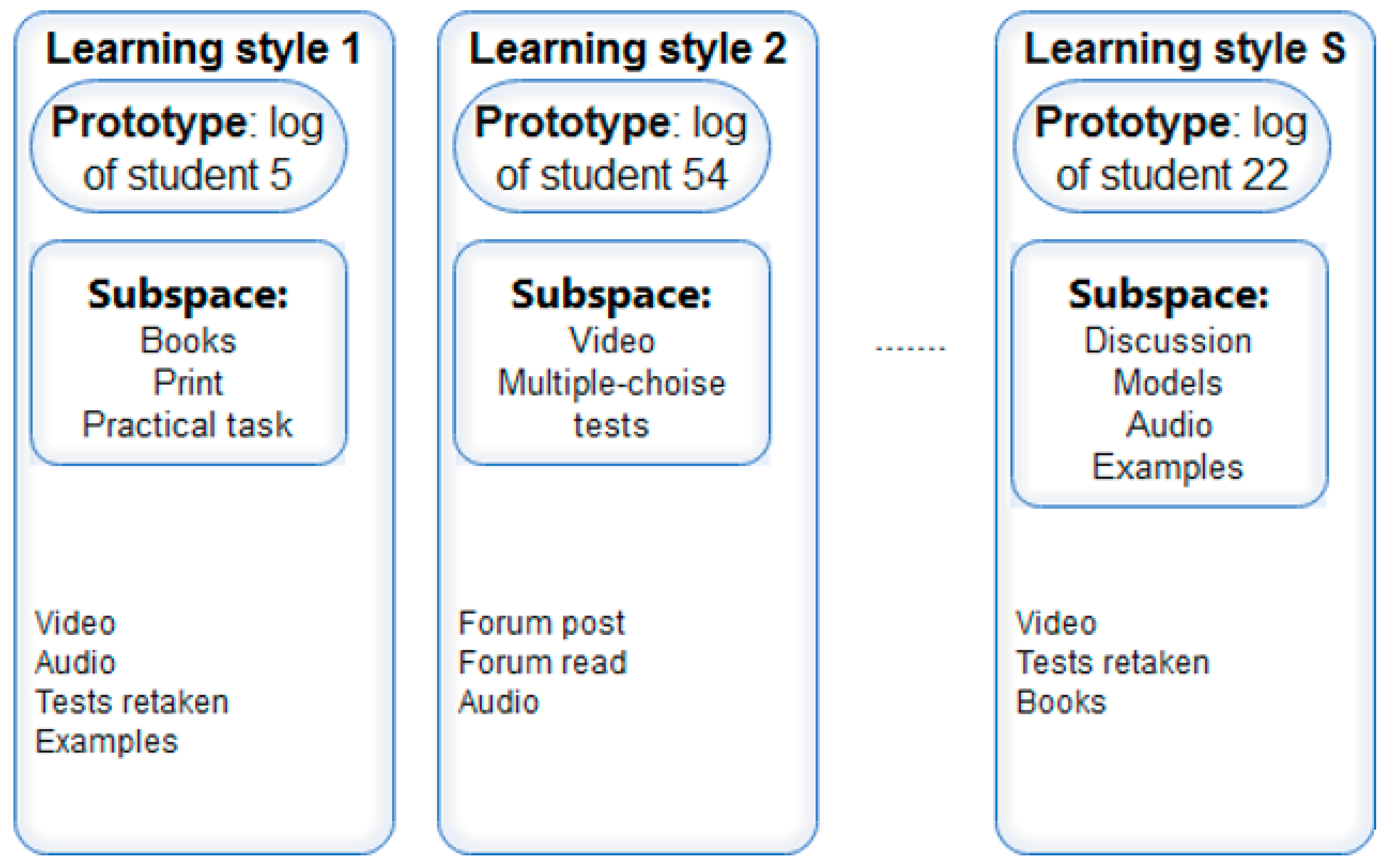
2.6.4. Interpretability

Machine learning algorithms build mathematical or/and statistical models based on sample data (“training data”). Relying on patterns and inference, these models make predictions, diagnoses, or decisions on specific tasks without using explicit instructions. Machine learning conditions improve products, processes, and research. However, computers usually do not explain their predictions, which is a barrier to the adoption of machine learning [53]. Interpretable models and methods for interpretation enabling humans to comprehend why certain decisions or predictions have been made were developed to cope with interpretability problems.

Authors in [53] define interpretability as the degree to which a human can understand the cause of a decision. Authors in [54] treat interpretability as the degree to which a human can consistently predict the model’s result. One can describe a model as interpretable if he/she can comprehend the entire model at once.

Authors in [55] point out that in explaining the predictions of a machine learning model, we rely on some explanation method, which is an algorithm that generates explanations. An explanation usually relates the feature values of an instance to its model prediction in a humanly understandable way [56]. The main questions are “What”, “How”, and “Why”; authors in [53] emphasize answers to “Why”. In spite of that, in some cases non-causal explanations exist (for example, answering the question ‘what happened’), and causality is the most important explanation; that is, an explanation should refer to causes. Probabilistic theories that BCM are based on state that event $\mathrm{X}$ is a cause of event $\mathrm{Y}$ if and only if the occurrence of $\mathrm{X}$ increases the probability of $\mathrm{Y}$ occurring.

BCM, which is proposed for students’ learning style diagnosis, uses exemplar-based explanations. It generates a prototype (example (actual data point) that best represents the cluster) and subspace (set of important features) for each cluster. In subspaces, the binary variable has value 1 for important features. Authors in [53] define a prototype as a data instance that is representative of all the data. In general, the importance of a feature is defined as the increase in the prediction error of the model after we permuted the feature’s values, which breaks the relationship between the feature and the true outcome [53]. There are permutation feature importance algorithms to train the feature importance. Depending on the purpose, they may use a training data set or test data set for training feature importance. Here it is necessary to emphasize the fundamental difference between generative and discriminative models, including the difference in the way it defines what important features are. As Kim Been explains, in BCM important features are whatever the particular cluster has in common (and also the rest has high likelihood in the entire generative process), and unimportant features are the ones where if they are changed arbitrarily, their cluster membership does not change. Thus, prototype and subspace form an explanation of a cluster. It is noteworthy again that in BCM, which uses an exemplar-based approach, an explanation consists of real data examples. For students’ learning style modelling using BCM, explanations for each cluster will consist of the following:

• prototype presented as log of behavioral activities of the student; this log best represents the cluster; in turn, a cluster represents learning style, and its features (for learning style modeling–behavioral activities) have cluster labels;
• subspace of important features, i.e., behavioral activities that have been performed most frequently in the virtual hypermedia learning environment by students whose learning style corresponds to the style represented by the cluster (Figure 4).

Besides prototypes, influential instances, criticisms, adversarial examples, etc., also may be used for explanations. Following [53], an instance is called “influential” when its deletion from the training data considerably changes the parameters or predictions of the model. In turn, criticism is a data instance that is not well represented by the set of prototypes. The purpose of criticisms is to provide insights together with prototypes, especially for data points that the prototypes do not represent well. Prototypes and criticisms can be used independently from a machine learning model to describe the data, but they can also be used to create an interpretable model or to make a black box model interpretable [53]. Authors in [54] describe an MMD-critic approach that combines prototypes and criticisms in a single framework. Maximum mean discrepancy (MMD) measures the discrepancy between two distributions [54]. MMD-critic uses the MMD statistic as a measure of similarity between data points and potential prototypes, and it efficiently selects prototypes that maximize the statistic. In addition to prototypes, MMD-critic selects criticism samples, i.e., samples that are not well-explained by the prototypes using a regularized witness function score [54]. Application of the MMD-critic approach may be usable in virtual learning environments for cases when, instead of personalization according to individual student’s learning style, the virtual learning environment needs to be automatically adapted to the learner model that is specific for most of students. Criticisms as explanations about what are not captured by prototypes could serve as indicators of students’ behavioral activities in the learning environment that are rare and therefore not worthy of attention (or worthy of exceptional attention, depending on specific task).

2.7. Comparative Analysis of Models and Networks

Results from the comparative analysis of models and methods are among the contributions of this paper to dynamic student learning style modelling; a short summary is presented in

Table 1. Comparative analysis of the models and methods using combined BN + CBR.

Criteria	BN/CBR	Optimized BN + CBR [30]	BCM [8,50,54,57,58]	Bayesian Patchworks [52]	Mixed Membership [57]
Model structure learning	heuristic algorithms	chi-squared test for construction of relationships between nodes and in case of change of number of nodes	generative mixture model, feature values exist in a discrete set that is not necessarily binary; uses clustering, number of clusters is previously defined	Bayesian hierarchical model, generative	generative statistical model, Latent Dirichlet allocation (LDA, standard mixture model); students are represented as random mixtures over latent learning styles, where each learning style is characterized by a distribution over all the behavioral activities in the student’s log
Features’ learning from data	expert-centric, data-centric	expert-centric, data-centric; effect centric	BCM uses generative story to explain parameters; generation of features is a result of a single prototype sharing its feature with the new observation; generation of features is correlated; collapsed Gibbs sampling being used converges quite quickly; After training the model, BCM cannot add new features	generation of features is a result of a vote among parents; generation of features is correlated	reverse-engineering the process where students’ logs are created by picking a set of learning styles and then for each learning style picking a set of behavioral activities; assumption that each feature value is generated independently;
Inference process	exact inference [59]: conditional probability tables’ update by marginal probability; using Bayes theorem; message passing algorithm	exact inference [59]: conditional probability tables’ update by marginal probability; using Bayes theorem; message passing algorithm on the subset of relevant nodes only	BCM is brute-force (proof by exhaustion, or proof by case analysis, complete induction); BCM makes joint approximate inference on latent and evidence variables; it uses Gibbs update, approximation of the posterior distribution using collapsed Gibbs sampling [59]	joint approximate inference on the selection of past cases that are influential to each new case, the subset of features of the past cases that are relevant to the new case, and how strong the influences of the past cases are on the new case; Metropolis-within-Gibbs sampling [59]; similar to nearest neighbors	variational Bayes approximation of the posterior distribution; alternative inference techniques use Gibbs sampling [59] and expectation propagation
Influence/effect on values of BN features/parameters	calculate the new (posterior) joint distribution of the network by conditioning it on the evidence	calculate the new (posterior) joint distribution of the network by conditioning it on the evidence	at cluster level, using prototype; BCM limits new cases to be compared with only certain learned past cases (the prototypes) [52]; BCM’s generation of features is a result of a single prototype sharing its feature with the new observation [52]; generation of features is correlated through clusters [52]	at individual (parents) level: the distribution of values for any feature is generated by parents; BPatch’s generation of features is a result of a vote among parents [52]; generation of features is correlated through parents [52]	cluster proportions’ level; LDA has a strong (and false) assumption that each feature value is generated independently [52]
Computation time; use of memory	learning BN is NP hard; depends on inference algorithm [59]	comparing with BN/CBR: reduced time of computation due to saving of previous cases and reuse of them thus avoiding calculation of inference repeatedly; and due to reduction of complexity (reduction of the number of nodes involved in the diagnosis process)	generative story: convergence to the true distribution is extremely slow	slightly slower than BCM; comparing to BN + CBR: much slower; more memory than BCM; suited for small datasets the total number of influential neighbors for each new case is a critical factor in the performance of the model	fast collapsed Gibbs sampling for LDA can be as much as 8 times faster than the standard collapsed Gibbs sampler for LDA
Prediction accuracy	±80%; prediction accuracy decreases with an increase of BN size	prediction accuracy greater that in BN/CBR due to saving of previous cases and reuse of them	high unsupervised clustering accuracy as a function of iterations; prediction accuracy comparable to or better than prior art for standard datasets, in BCM classification accuracy was 85.9% [8,51]; prediction accuracy better than in LDA	high; classification accuracy depends on hyperparameters	±80%;
Handling missing data points	two main approaches for learning BN parameters are Expectation-Maximization (EM) and a simulation-based Gibbs sampler called Data Augmentation (DA) [60]. The Expectation step involves the performance of inference in order to obtain sufficient statistics. In Maximization step the Maximum Likelihood (ML) estimates are computed from the sufficient statistics. These two steps are iterated until the parameter estimates converge [61]. Data Augmentation is similar, but it is non-deterministic. Instead of calculating expected statistics, a value is drawn from a predictive distribution and imputed. Similarly, instead of calculating the ML estimates, draws from the posterior distribution on the parameter space (conditioned on the sufficient statistics of the most recent imputed dataset) are made. Based on Markov chain Monte Carlo theory, this will eventually return realizations from the posterior parameter distribution [61]. Other: Bound and Collapse (BC) approach; structural EM (SEM); eMC3; eMC4 (importance sampling, that does not require exact inference in a BN; specifying an approximate distribution is cheaper than a perfect one) [61]. When data are missing at random, Multivariate Imputation by Chained Equations (MICE) method may be applied [62]. It imputes data on a variable-by-variable basis by specifying an imputation model per variable [62]. Depending on the nature of the data, Random forest, a non-parametric imputation method, may be applicable to various variable types that works well with both data missing at random and not missing at random [62]. In some cases, list-wise or pair-wise deletion of the missing observations can be used or other methods may be applied [63]		BCM will ignore missing features and only focus on what is common between data points explicitly for clustering or cluster all data points with missing feature (-s) in one cluster-existing Bayesian Case model [8,51] is not targeted for missing data	any method for imputation may be used. Besides that, for each dimension of features, an artificial output representing missing value can be added	implementations of latent class (LC) models (i.e., mixture models that describe the distribution of categorical data) for multiple imputation (MI) [34]: The Maximum Likelihood LC model (MLLC), the standard Bayesian LC model (BLC), the Divisive LC model (DLC), and the Dirichlet Process Mixture of Multinomial distributions (DPMM)
Explanations	heuristic and normative methods exist for BN explanations. According to [64], there are the following types of explanations: explanations of evidence (abduction: Pearl’s propagation, linear restrictions system, weighted Boolean function acyclic directed graph, genetic algorithm based or stochastic annealing based approximate abduction), explanations of model (static explanations, containing information in data base) and explanations of reasoning at micro and macro levels (dynamic explanations: reasoning process that produced results; explanations why the network did not produce expected results; hypothetical reasoning)) [64]. Verbal, graphical, multimedia explanations may be presented. As CBR represents domain knowledge-oriented method, general domain model combined with CBR enables to generate targeted explanations for the user as well as for its internal reasoning process [27]. Typically, BN + CBR generate explanations given the observed symptoms. CBR models designed explicitly to produce explanations rely on the backward chaining of the causal relation from a solution, which does not scale as complexity increases [8,51]; other CBR models require to be created by experts;		in BCM, the underlying structure of the observations is represented by a standard discrete mixture model. Explanations produced by mixture models are typically presented as distributions over features [8,51]. BCM uses generative story to explain parameters. BCM preserves the power of CBR in generating interpretable output, where interpretability comes not only from sparsity but from the prototype exemplars [8,51]. Explanations are based on natural exemplars: a prototype and a set of important features defining a cluster [8,51];	model provides explanations that are similar to the way the reasons are presented naturally. Deep insights into data	explanations presented as distributions over features. LDA represents documents as mixtures of topics that spit out words with certain probabilities. It is a way of automatically discovering topics that documents contain–LDA finds a set of topics that are likely to have generated the collection of documents
Scalability	high number of features and complexity hinder performance of BN. CBR improves BN performance, reducing the complexity	No restrictions on network size and topology	in BCM, Gibbs sampling [65] inference technique is used to perform inference. However, there are other techniques that may scale better for larger datasets (e.g., variational inference, tensor decomposition methods). Since not all distributions used in BCM are within the exponential families (exponential distribution is a case of the gamma distribution, and it is a memoryless distribution), the current BCM model does not offer closed-form updates (i.e., updates that can be evaluated in a finite number of operations, solved analytically) when using variational inference. Modification or approximation of the BCM model may ease the derivation of variational inference [8,51]	generally, patchwork is a distributed density clustering algorithm with linear computational complexity and linear horizontal scalability. Bayesian Patchworks may be treated as a form of adaptive k nearest neighbors. Each case is generated by several neighbors, each using a different distance measure to the present case. Considering neighbors through different lenses makes more sense than fixing one distance measure, and having only one way to search for nearest neighbors [52]	variational inference, F + LDA, F + Nomad LDA, Alias LDA, Light LDA, Warp LDA, LDA* or other methods should be used instead of Gibbs sampling for large data sets and/or scalable and efficient distribution of the computation across multiple machines [66]

. A comparative analysis was conducted bearing in mind the purpose to apply CBR and BN in combination for student learning style identification. In making a choice from the below-mentioned variants for dynamic student learning style modelling, the properties specified in Table 1 should be considered as minimum.

Results of the comparative analysis highlighted that for modelling based on large, discrete data sets, BCM is the best choice as it converges faster than Bayesian patchworks, its prediction accuracy is high, and it has human-understandable explanations. For BCM, the effect on values of features is at cluster (not individual) level; therefore, BCM is relevant for students’ learning style modelling based on generation of learning style clusters.

3. Discussion

During our systematic review of the literature on the combination of BN and CBR, two main trends for modeling student learning style, based on student’s behavior in virtual learning system, were highlighted. Both of them also can have some variations (for example, using (or not) student’s feedback, having (or not) the possibility to change/remove features that influence learning style, optimizing (or not) message propagation in BN, using different models for case representation or using different similarity measures, etc.). The first trend is based on employment of a simple or optimized Bayesian network and CBR, combining these two by a common parameter space. This approach is reasonable for cases when BN is constructed by experts, using the learning style model known in advance (for example, Felder–Silverman learning styles model). Using the first approach, inferences about the dominate learning style of the student can be made, and proportions of student styles according to the learning style model chosen can be concluded.

The second approach (using BCM) does not use a previously defined learning style model; for each student, a model is generated from his/her behavioral data or students’ past cases’ data. BCM preserves the power of CBR in generating interpretable output, where interpretability comes not only from sparsity but from the prototype exemplars. According to recent publications of authors who systematized methods being used in dynamic learning style identification (for example [32,67]), and to the best of our knowledge, BCM has never been applied for modelling learning style in adaptive hypermedia learning systems. Thus, application of an exemplar-based Bayesian case model using combined CBR + BN for student’s learning style modelling is new.

For both approaches, having information about the student’s learning style and using corresponding scenarios of possible adaptations of the virtual learning environment, the virtual learning environment can be personalized in a way that best fits the particular student.

In spite of that, this paper has no intention of describing the modeling of student learning styles using a Bayesian hierarchical model, but we must note that this option should be suitable for modeling student learning styles. The Bayesian hierarchical model models data from several subjects, and different parameter values may be characteristic to the individual models of each subject. In the Bayesian hierarchical model some parameters are partly determined, and the model can infer these parameters from data, i.e., from individual distributions defined by other parameters. The tension between fitting each subject as well as possible (optimal choice of individual parameters) and fitting the group as a whole exists in the Bayesian hierarchical model. This tension results in a movement of the individual parameters toward the group mean, given that we do not desire to over fit the data, and we fit the noise in each individual’s data [68]. Thus, both the information in posterior distributions over parameters and posterior predictive distributions over data provide direct information about how a model accounts for data [68]. Using the property of the Bayesian hierarchical model that the joint posterior carries more information than the individual marginal distributions, and presuming that for modeling student learning styles we have individual models with their own parameters for each student, the hierarchical Bayesian model may also be seen as a way for modelling a learning style characteristic for all students (or a group of students) and/or for inferring individual student learning styles.

4. Comparing Performances of LDA and BCM

In this section, we discuss the performances of the LDA and BCM.

Linear discriminant analysis (LDA) is a generalization of Fisher’s linear discriminant. It finds a linear combination of features that characterizes or separates two or more classes. It may be used as a linear classifier or for dimensionality reduction before classification. Unlike discriminative machine learning techniques that tend to be useful primarily for binary classification, LDA described in this paper is appropriate for multi-class domains [67]. Following [67], the insight behind LDA is that the k − 1 dimensional subspace connecting the centroids of each class provides a simpler reduced manifold to make decisions, where k is the number of different image classes. LDA as a classification algorithm is unsupervised in that there is no need to label data, just a prior distribution is needed as it is a Bayesian model. Since precision and recall necessarily depend on the true classes, they cannot be directly applied to an unsupervised method. It is possible to evaluate clustering methods, but accuracy is not a correct criterion. Thus, it is not appropriate to use accuracy as performance criterion for LDA. In order to compare BCM prediction accuracy with LDA, the BCM-learned cluster labels are provided as features to a supervised learning model, support vector machine (SVM) with linear kernel [8], i.e., the mixture vector π from BCM can be used as a feature of length S for input to other classification methods, such as SVM or logistic regression [8]. Then, SVM is trained on the low-dimensional representations provided by LDA, and both SVNs are compared. It is known from the literature that the prediction accuracy when using the full dataset acquired by LDA matches that for the same dataset when using a combined LDA and SVM approach [8]. It was identified from the literature, mainly [8], that BCM’s accuracy is better than that produced by LDA: 0.76 ± 0.017 vs. 0.77 ± 0.03. The improved accuracy of BCM over LDA is explained in part by the ability of BCM to capture dependencies among features via prototypes, data points with a label in the given datasets [8]. Furthermore, comparing Bayesian patchworks’ accuracy with that of BCM, an improvement in accuracy continues to be observed [53] (

Table 2. Comparison of accuracy produced by LDA, BCM, and Bayesian patchworks [8,51].

LDA	BCM	Bayesian Patchworks
0.76	0.77	0.83

).

5. Conclusions

BCM is proposed for learning style identification. Application of BCM for diagnosing student learning styles is new. To the best of our knowledge, BCM has never been applied for modelling learning styles in adaptive hypermedia learning systems. Using BCM, each learner will be assigned the highest probable cluster that corresponds to the learning style represented by actual co-occurring behavioral activities in VLE.

Student learning styles predicted by BCM may be used for learning personalization: learning content adaptation (presentation of the content that fits the learner’s learning style), presentation of personal instructions, recommendation of learning material in the form that is preferred by the particular student, creation of learning scenarios according to student’s needs, etc. Clusters generated by BCM might be used not only for personalization of the virtual learning environment according to the student’s needs (hypermedia learning systems could automatically adapt according to the student’s learning style identified by BCM), but also by teachers helping them to prepare versions of courses relevant to prototypes and important features of particular clusters. Having clusters of learning styles based on actual student behavioral data, teachers or instructors would be presented the possibility to prepare learning courses that meet individual needs of students.

As in most cases few learning styles are intrinsic to the same student, LDA might also be usable for identification of proportions of student learning styles. In this case, dominant learning styles will be assigned to each student according to data from his/her logs consisting of his/her behavioral activities in VLE.

Further research trends should explore, more in depth, mechanisms for incorporating learner’s feedback into student learning style models. Experimental BCM applications for identifying student learning styles are also intended.

References

1. Kurilovas, E. On Data-Driven Decision-Making for Quality Education. Comput. Hum. Behav. 2020, 207, 105774. [Google Scholar] [CrossRef]
2. Jevsikova, T.; Berniukevičius, A.; Kurilovas, E. Application of Resource Description Framework to Personalise Learning: Systematic Review and Methodology. Inform. Educ. 2017, 16, 61–82. [Google Scholar] [CrossRef]
3. Kurilovas, E.; Dagiene, V. Computational Thinking Skills and Adaptation Quality of Virtual Learning Environments for Learning Informatics. Int. J. Eng. Educ. 2016, 32, 1596–1603. [Google Scholar]
4. Kurilovas, E.; Kurilova, J.; Andruskevic, T. On Suitability Index to Create Optimal Personalised Learning Packages. In Proceedings of the International Conference on Information and Software Technologies, Druskininkai, Lithuania, 13–15 October 2016. [Google Scholar]
5. Kurilovas, E. Advanced Machine Learning Approaches to Personalize Learning: Learning Analytics and Decision Making. Behav. Inf. Technol. 2019, 38, 410–421. [Google Scholar] [CrossRef]
6. Kim, B.; Glassman, E.; Johnson, B.; Shah, J. iBCM: Interactive Bayesian case model empowering humans via intuitive interaction. In Computer Science and Artificial Intelligence Laboratory Technical Report; DSpace@MIT, Massachusetts Institute of Technologies: Cambridge, MA, USA, 2015. [Google Scholar]
7. Richter, M.M.; Weber, R.O. Case-Based Reasoning: A Textbook; Springer: Berlin, Germany, 2013; ISBN 978-3-642-40167-1. [Google Scholar]
8. Kim, B. Interactive and Interpretable Machine Learning Models for Human Machine Collaboration. Ph.D. Thesis, Massachusetts Institute of Technology, Cambridge, MA, USA, 2015. [Google Scholar]
9. Aamodt, A.; Plaza, E. Case-Based Reasoning: Foundational Issues, Methodological Variations, and System Approaches. AI Commun. 1994, 7, 39–59. [Google Scholar] [CrossRef]
10. Costa, M.; Sousa, O.; Neves, J. Managing Legal Precedents with Case Retrieval Nets. 1999. Available online: http://jurix.nl/pdf/j99-02.pdf (accessed on 14 March 2021).
11. Forbus, K.; Gentner, D.; Law, K. MAC/FAC: Model of similarity-based retrieval. Cogn. Sci. 1995, 19, 141–205. [Google Scholar] [CrossRef]
12. Kramer, A. Introduction to Bayesian Inference. 2016. Available online: https://www.datascience.com/blog/introduction-to-bayesian-inference-learn-data-science-tutorials (accessed on 7 January 2021).
13. Stack Exchange. 2018. Available online: https://stats.stackexchange.com/questions/307882/why-is-it-necessary-to-sample-from-the-posterior-distribution-if-we-already-know (accessed on 7 January 2021).
14. Doll, T. LDA Topic Modeling: An Explanation. 2018. Available online: https://towardsdatascience.com/lda-topic-modeling-an-explanation-e184c90aadcd (accessed on 14 March 2021).
15. Liu, S. Latent Dirichlet Distribution. 2019. Available online: https://towardsdatascience.com/dirichlet-distribution-a82ab942a879 (accessed on 14 March 2021).
16. Stack Exchange. Bayesian Updating without Conjugate Prior. 2013. Available online: https://stats.stackexchange.com/questions/45371/bayesian-updating-without-conjugate-prior?rq=1 (accessed on 14 March 2021).
17. Hewitt, L. Bayesian Inference in Generative Models. 2018. Available online: https://www.youtube.com/watch?v=PRY2NbOXbHk (accessed on 14 March 2021).
18. Franzen, J. Bayesian Inference for a Mixture Model Using the Gibbs Sampler. 2006. Available online: http://gauss.stat.su.se/rr/RR2006_1.pdf (accessed on 14 March 2021).
19. Quora. Why Is LDA a Mixture Model. Available online: https://www.quora.com/Why-is-LDA-a-mixture-model (accessed on 14 March 2021).
20. Grosse, R.; Srivastava, N. Lecture 16: Mixture Models. 2018. Available online: http://www.cs.toronto.edu/~rgrosse/csc321/mixture_models.pdf (accessed on 14 March 2021).
21. r/learnmath-Explain to Me Like I’m Five: Gibbs Sampling. 2012. Available online: https://www.reddit.com/r/learnmath/comments/x4pqe/explain_to_me_like_im_five_gibbs_sampling/ (accessed on 14 March 2021).
22. Bruland, T.; Aamodt, A.; Langseth, H. Architectures Integrating Case-Based Reasoning and Bayesian Networks for Clinical Decision Support. In Proceedings of the Intelligent Information Processing V—6th IFIP TC 12 International Conference, Manchester, UK, 13–16 October 2010. [Google Scholar]
23. Prentzas, J.; Hatzilygeroudis, I. Case-based reasoning integration: Approaches and applications. In Case-Based Reasoning: Processes, Suitability and Applications; Nova Science Publishers: New York, NY, USA, 2011; pp. 1–28. [Google Scholar]
24. Marling, C.; Sqalli, M.; Rissland, E.; Munoz-Avila, H.; Aha, D. Case-based reasoning integrations. AI Mag. 2002, 23, 69. [Google Scholar] [CrossRef] [Green Version]
25. Houeland, T.; Bruland, T.; Aamodt, A.; Langseth, H. A Hybrid Meta Reasoning Architecture Combining Case-Based Reasoning and Bayesian Networks; Semantic Scolar, Allen Institute for AI: Seattle, WA, USA, 2011. [Google Scholar]
26. Schiaffino, S.; Amandi, A. User profiling with case-based reasoning and Bayesian networks. In Proceedings of the International Joint Conference IBERAMIA-SBIA 2000, Atibaia, Brazil, 19–22 November 2000; pp. 12–21. [Google Scholar]
27. Nikpour, H. Prediction and explanation by combined model-based and case-based reasoning. In Proceedings of the Twenty-Fourth International Conference on Case-Based Reasoning (ICCBR 2016), Atlanta, GA, USA, 31 October–2 November 2016. [Google Scholar]
28. Nikpour, H.; Aamodt, A.; Bach, K. Bayesian-Supported Retrieval in BNCreek: A Knowledge-Intensive Case-Based Reasoning System. In Case-Based Reasoning Research and Development; Springer: Cham, Switzerland, 2018; pp. 323–338. [Google Scholar]
29. Gonzalez, K.; Burguillo, J.C.; Llamas, M. A qualitative comparison of techniques for student modelling in intelligent tutoring systems. In Proceedings of the Frontiers in Education, 36th Annual Conference, San Diego, CA, USA, 27–31 October 2006. [Google Scholar]
30. Bannacer, L.; Ciavaglia, L.; Chibani, A.; Amirat, Y. Optimization of fault diagnosis based on the combination of Bayesian networks and case-based reasoning. In Proceedings of the 2012 IEEE Network Operations and Management Symposium, Maui, HI, USA, 16–20 April 2012. [Google Scholar]
31. Aamodt, A.; Langseth, H. Integrating Bayesian networks into knowledge intensive CBR. In AAAI Technical Report WS-98-15; AAAI: Palo Alto, CA, USA, 1998. [Google Scholar]
32. Khamparia, A. Knowledge and intelligent computing methods in e-learning. Int. J. Technol. Enhanc. Learn. 2015, 7, 221–242. [Google Scholar] [CrossRef]
33. Ferreira, L.D.; Spadon, G.; Carvalho, A.C.; Rodrigues, J.F. A comparative analysis of the automatic modeling of Learning Styles through Machine Learning techniques. In Proceedings of the 2018 IEEE Frontiers in Education Conference (FIE), San Jose, CA, USA, 3–6 October 2018. [Google Scholar]
34. Vidotto, D.; Kaptein, M.C.; Vermunt, J.K. Multiple Imputation of Missing Categorical Data using Latent Class Models: State of the Art. Psychol. Test Assess. Model. 2015, 57, 542. [Google Scholar]
35. Neal, R.M. Bayesian mixture modeling by Monte Carlo simulation. In Technical Report CRG-TR-91-2; Computer Science, University of Toronto: Toronto, ON, Canada, 1991. [Google Scholar]
36. Celeux, G.; Kamry, K.; Malsiner-Walli, G.; Marin, J.-M.; Robert, C. Computational Solutions for Bayesian Inference in Mixture Models. 2018. Available online: https://www.researchgate.net/publication/329772148_Computational_Solutions_for_Bayesian_Inference_in_Mixture_Models (accessed on 14 March 2021).
37. While My MCMC Gently Samples, Bayesian Modelling, Data Science and Phython. MCMC Sampling for Dummies. 2015. Available online: https://twiecki.io/blog/2015/11/10/mcmc-sampling/ (accessed on 7 January 2021).
38. Dwivedi, P. Doing Cool Things with Data. NLP: Extracting the Main Topics from Your Dataset Using LDA in Minutes. 2018. Available online: https://towardsdatascience.com/nlp-extracting-the-main-topics-from-your-dataset-using-lda-in-minutes-21486f5aa925 (accessed on 14 March 2021).
39. Gormley, M. Dirichlet process and Dirichlet process mixtures. In Probabilistic Graphical Models; School of Computer Science, Carnegie Mellon University: Pittsburgh, PA, USA, 2016. [Google Scholar]
40. Blei, D.; Ng, A.; Jordan, M. Latent Dirichlet allocation. J. Mach. Learn. Res. 2003, 3, 993–1022. [Google Scholar]
41. De Paulo Faleiros, T.; de Andrade Lopes, A. On the equivalence between algorithms for non-negative Matrix Factorization and Latent Dirichlet Allocation. In Proceedings of the International Conference on Computational Science and Its Applications, Trieste, Italy, 3–6 July 2017. [Google Scholar]
42. Airoldi, E.M.; Blei, D.M.; Erosheva, E.A.; Fienberg, S.E. Introduction to Mixed Membership Models and Methods. Handb. Mix. Membsh. Model. Appl. 2020, 100, 3–14. [Google Scholar]
43. Shalizi, C. Mixture Models. 2020. Available online: https://www.stat.cmu.edu/~cshalizi/uADA/12/lectures/ch20.pdf (accessed on 10 June 2021).
44. About: Plate Notation. 2019. Available online: http://dbpedia.org/page/Plate_notation (accessed on 19 January 2021).
45. Zinkov, R. Stop Using Plate Notation. 2013. Available online: https://www.zinkov.com/posts/2013-07-28-stop-using-plates/ (accessed on 7 January 2021).
46. Lu, S.; Yu, L.; Feng, S.; Zhu, Y.; Zhang, W.; Yu, Y. CoT: Cooperative Training for Generative Modeling of Discrete Data. In Proceedings of the ICLR 2019 Conference, New Orleans, LA, USA, 6–9 May 2019. [Google Scholar]
47. Neal, R.M. Markov chain sampling methods for Dirichlet process mixture models. J. Comput. Graph. Stat. 2000, 9, 249–265. [Google Scholar]
48. Wikipedia. Maximum Entropy Probability Distribution. 2019. Available online: https://en.wikipedia.org/wiki/Maximum_entropy_probability_distribution (accessed on 14 March 2021).
49. Liu, J.S. The Collapsed Gibbs Sampler in Bayesian Computations with Applications to a Gene Regulation Problem. J. Am. Stat. Assoc. 1994, 89, 958–966. [Google Scholar] [CrossRef]
50. Goštautaitė, D. Recommendation systems and recommendation dashboards for learning personalization. In Proceedings of the INTED2019—13th International Technology, Education and Development Conference, Valencia, Spain, 11–13 March 2019. [Google Scholar]
51. Kim, B.; Rudin, T.; Sah, J. The Bayesian CASE model: A generative approach for case-based reasoning and prototype classification. In Proceedings of the Neural Information Processing Systems, Montreal, QC, Canada, 8–13 December 2014. [Google Scholar]
52. Moghaddass, R.; Rudin, C. Bayesian Patchworks: An Approach to Case-Based Reasoning. 2018. Available online: https://arxiv.org/abs/1809.03541v1 (accessed on 14 March 2021).
53. Molnar, C. Interpretable Machine Learning. A Guide for Making Black Box Models Explainable. Creative Commons Attribution-NonCommercial-ShareAlike 4.0 International License. 2019. Available online: https://christophm.github.io/interpretable-ml-book/index.html (accessed on 12 May 2021).
54. Kim, B.; Khanna, R.; Koyejo, O.O. Examples are not enough, learn to criticize! Criticism for interpretability. In Proceedings of the NIPS’16: 30th International Conference on Neural Information Processing Systems, Barcelona, Spain, 5 December 2016. [Google Scholar]
55. Garg, V.K.; Wang, Y. Signal Types, Properties, and Processes. In The Electrical Engineering Handbook; Academic Press: New York, NY, USA, 2005. [Google Scholar]
56. Miller, T. Explanation in Artificial Intelligence: Insights from the Social Sciences. 2018. Available online: https://arxiv.org/pdf/1706.07269.pdf (accessed on 12 May 2021).
57. Quora. What Is the Good Explanation of HDP Latent Dirichlet Allocation. 2015. Available online: https://www.quora.com/What-is-the-good-explanation-of-HDP-latent-Dirichlet-allocation (accessed on 14 March 2021).
58. Kim, B. Bayesian CASE Model—Generative Approach for Case-Based Reasoning and Prototype Classification. 2015. Available online: https://www.youtube.com/watch?v=xSViWMPF7tE (accessed on 19 January 2021).
59. Guo, H.; Hsu, W. A Survey of Algorithms for Real-Time Bayesian Network Inference. In AAAI Technical Report WS-02-15; AAAI: Palo Alto, CA, USA, 2002. [Google Scholar]
60. Biostatistics and Medical Informatics. Learning Bayesian Networks. 2018. Available online: http://pages.cs.wisc.edu/~dpage/cs760/BNall.pdf (accessed on 12 May 2021).
61. Riggelsen, C.; Feelders, A. Learning Bayesian Network Models from Incomplete Data using Importance Sampling. In Proceedings of the Tenth International Workshop on Artificial Intelligence and Statistics, Bridgetown, Barbados, 6–8 January 2005. [Google Scholar]
62. Rai, S.S. 3 Methods to Handle Missing Data. 2019. Available online: https://www.datascience.com/blog/missing-data-imputation (accessed on 10 May 2021).
63. Sauro, J. 7 Ways to Handle Missing Data. 2015. Available online: https://measuringu.com/handle-missing-data/ (accessed on 12 May 2021).
64. Lacave, C.; Diez, F.J. A review of explanation methods for Bayesian networks. Knowl. Eng. Rev. 2002, 17, 107–127. [Google Scholar] [CrossRef]
65. Tomar, A. Machine Learning. Topic Modelling Using LDA and Gibbs Sampling Explained. 2018. Available online: https://medium.com/@tomar.ankur287/topic-modeling-using-lda-and-gibbs-sampling-explained-49d49b3d1045 (accessed on 7 January 2021).
66. Yu, H.F.; Hsieh, C.J.; Dhillon, I. Fast and Scalable Algorithms for Topic Modeling. 2015. Available online: https://bigdata.oden.utexas.edu/project/scalable-topic-modeling/ (accessed on 12 May 2021).
67. Mohanty, N.; Rath, T.M. Handbook of Statistics; Elsevier: Amsterdam, The Netherlands, 2013. [Google Scholar]
68. Shiffrin, R.M.; Lee, M.D.; Kim, W.; Wagenmakers, E.J. A Survey of Model Evaluation Approaches with a Tutorial on Hierarchical Bayesian Methods. Cogn. Sci. 2008, 32, 1248–1284. [Google Scholar] [CrossRef] [PubMed]
Figure 1. Bayesian case model: graphical representation in Plate notation [8].
Applsci 11 07083 g001
Figure 2. Generation of students’ learning style clusters represented by prototype and important Figure 3.
Applsci 11 07083 g002
Figure 3. Bayesian case model [51] for students’ learning style prediction.
Applsci 11 07083 g003
Figure 4. Example of BCM explanations for learning styles.
Applsci 11 07083 g004