Article

A Decoupling Strategy for Reliability Analysis of Multidisciplinary System with Aleatory and Epistemic Uncertainties

1
School of Mechanical Engineering and Automation, Beihang University, Beijing 100191, China
2
Beijing Institute of Mechanical and Electrical Engineering, Beijing 100072, China
*
Author to whom correspondence should be addressed.
Appl. Sci. 2021, 11(15), 7008; https://doi.org/10.3390/app11157008
Submission received: 1 July 2021 / Revised: 22 July 2021 / Accepted: 26 July 2021 / Published: 29 July 2021
(This article belongs to the Special Issue Uncertainty Analysis of Mechanical Systems)

Abstract

:
In reliability-based multidisciplinary design optimization, both aleatory and epistemic uncertainties may exist in multidisciplinary systems simultaneously. The uncertainty propagation through coupled subsystems makes multidisciplinary reliability analysis computationally expensive. In order to improve the efficiency of multidisciplinary reliability analysis under aleatory and epistemic uncertainties, a comprehensive reliability index that has clear geometric meaning under multisource uncertainties is proposed. Based on the comprehensive reliability index, a sequential multidisciplinary reliability analysis method is presented. The method provides a decoupling strategy based on performance measure approach (PMA), probability theory and convex model. In this strategy, the probabilistic analysis and convex analysis are decoupled from each other and performed sequentially. The probabilistic reliability analysis is implemented sequentially based on the concurrent subspace optimization (CSSO) and PMA, and the non-probabilistic reliability analysis is replaced by convex model extreme value analysis, which improves the efficiency of multidisciplinary reliability analysis with aleatory and epistemic uncertainties. A mathematical example and an engineering application are demonstrated to verify the effectiveness of the proposed method.

1. Introduction

With progress in science and technology, the focus on the effect of uncertainty has received increasing attention in engineering design. As an indispensable ingredient of reliability-based multidisciplinary design optimization (RBMDO), the multidisciplinary reliability analysis (MRA) plays a decisive role in evaluating the reliability of multidisciplinary systems. In RBMDO, the probabilistic model on basis of a large amount of statistical data is the most common method to quantify aleatory uncertainty and it has achieved great success [1,2]. With the development of artificial intelligence technology, some machine learning and advanced statistical framework, such as probability boxes [3], are introduced into the field of reliability evaluation. Xiang et al. [4] proposed a deep reinforcement learning-based sampling method for reliability analysis, which uses a deep neural network as agent to select test points automatically and construct the surrogate model for reliability assessment. Ghoreishi et al. [5] proposed a Bayesian surrogate learning for reliability analysis, which increases the minimum number of possible samples from various disciplines to achieve accurate and reliable uncertainty propagation in coupled multidisciplinary systems. These methods all need enough statistical information.
However, the lack of statistical data often makes it difficult to quantify the statistical distribution of the design parameters. It is incapable of obtaining credible results for a probabilistic model, so non-probabilistic models such as convex models are used to quantify single interval uncertainty. Actually, uncertainties are ubiquitous in each design stage of complex engineered systems, which can be classified into aleatory uncertainty (AU) and epistemic uncertainty (EU) according to human cognition [6]. Aleatory uncertainty is also known as random uncertainty, stochastic uncertainty and irreducible uncertainty. It describes the internal changes of the physical system and has sufficient test data and perfect information. Conversely, the epistemic uncertainty is affected by negligence, experimental conditions or other cognitive ability caused by the lack of knowledge and imperfect information, so it is also known as reducible uncertainty, subjective uncertainty, etc. Many scholars have studied some reliability analysis methods considering interval or other epistemic uncertainties. Fuzzy theory [7], possibility theory [8], evidence theory [9] and convex set theory [10] have been used to quantify epistemic uncertainty and to conduct reliability analysis.
In many circumstances, both aleatory and epistemic uncertainties coexist in the complex and coupled multidisciplinary systems. According to different analysis principles, the current reliability analysis methods under mixed uncertainties can be divided into “transformation type” and “analysis type”. “Transformation type “refers to transforming different uncertainty variables into the same type of uncertainty variables, and then using the reliability analysis method under a single type of uncertainty for analysis. Researchers such as Du et al. [11] transformed random variables into fuzzy variables according to the principle of probability possibility consistency and the most conservative condition. Shah et al. [12] used evidence theory and random expansion method to study the uncertainty of implicit state when random variables and interval variables exist at the same time. While, “analysis type” refers to the analysis of system reliability by different uncertainty quantification theories without any transformation for the mixed uncertainties. Researchers such as Huang et al. [13] have established the conditional possibility model of failure based on probability/possibility theory, and analyzed the reliability based on the principle of cut set.
For a multidisciplinary system, due to the coupling between disciplines, uncertainty will spread among disciplines, so it is necessary to combine reliability analysis method with multidisciplinary optimization strategy [14], but the direct integration of reliability analysis method and multidisciplinary design optimization (MDO) strategies is inefficient when solving large-scale MDO problems, because when both aleatory and epistemic uncertainties are involved, the procedure of direct integration method will become a nested three-layer loop. Therefore, Meng [15] proposed an efficient uncertainty-based design optimization strategy with random and interval variables for multidisciplinary engineering systems. The method evaluates the uncertainty constraints in the worst case, but it cannot evaluate the impact of interval uncertainties on the design space.
For this purpose, the methods proposed in this paper mainly studies from two following aspects: (1) considering the multisource uncertainties, a multidisciplinary reliability comprehensive evaluation index with clear geometric meaning is proposed. It is pointed out that the reliability should be an interval rather than a single value under the condition of aleatory and epistemic uncertainties. The minimum value of the reliability interval is used as the measurement standard, and the interval difference directly reflects the influence of epistemic uncertainties on the limit state function. (2) Based on the comprehensive evaluation index, a decoupling strategy for multidisciplinary reliability approach under multisource uncertainties (MU-DBMRA) is proposed, which divide the three-layer nested loop of MRA process into a sequential monocyclic process, consisting of multidisciplinary probabilistic reliability analysis (MPRA), multidisciplinary convex reliability analysis (MCRA) and multidisciplinary analysis (MDA). Results of example analysis indicate that the proposed method can solve decoupling problems of MRA process in a proper way, and greatly improve efficiency of MRA.
This paper is constructed as follows: the first section introduces the related works of uncertainty quantification and PMA principle used in this paper; the second section introduces principle and algorithm flow of the proposed method under multisource uncertainties. Section 3 presents one numerical example and one engineering design example for demonstration. Section 4 concludes and presents possible future work.

2. Related Works

2.1. Mixed Uncertainties Quantification Based on Probability Theory and Convex Set Theory

In order to make the best use of uncertainties, both the probability and convex set theories are employed to quantify the aleatory and epistemic uncertainties respectively. The multi-ellipsoid convex model [16] is adopted to quantify the epistemic uncertainty. The epistemic uncertainty involved in this paper refers to the interval uncertainty.
When there are enough data or information for the design variables, they can be modeled using the probability theory. The normal random variable x can be transformed into a standard normal random variables u by:
u = ( x x ¯ ) σ
where x ¯ and σ are the mean value and the standard deviation of x, respectively.
Generally, the aleatory variables x can be transformed to a set of uncorrelated normal variables via the Rosenblatt transformation [17]. This transformation from x to u is based on the condition that the cumulative distribution functions (CDF) of the random variables remain the same before and after the transformation. The transformation can be expressed by
F X i ( x i ) = Φ ( u i ) , i = 1 , 2 , , n
where Φ(•) is the (cumulative distribution functions) CDF of the standard normal distribution.
Then, the transformed standard normal variable can be denoted as
u i = Φ 1 [ F X i ( x i ) ]
For example, the normally distributed random variable xi~N(μi, σi) and the transformed ui can be obtained with Equation (4).
u i = Φ 1 [ F X i ( x i ) ] = Φ 1 [ Φ ( x i μ i σ i ) ] = x i μ i σ i
where Φ−1(•) is the inverse standard normal cumulative distribution function. As a result, all the random variables can be transformed into independent standard normal ones in u space.
For the quantification of epistemic uncertainties, scholars have also made a lot of attempts and innovations. In this paper, a convex model, which has a clear concept, simple model and straightforward multiple variables, is used to quantify epistemic uncertainties. When dealing with variables, convex model requires less uncertain information and only needs to know its disturbance range.
Ellipsoidal convex model, referred to as ELP model, can be expressed as follows:
Ω S E L P = { α ( t ) R r : [ α α ¯ ] T W [ α α ¯ ] θ 2 }
where α is the uncertainty parameter to be described, W is a weighted matrix, which reflects the correlation between different variables; θ is the radius of the ellipsoid, which reflects the disturbance range and degree of uncertainties; α ¯ express the nonzero principal value (or mean value) of α. For the convenience of processing, the epistemic uncertainty variables quantized by convex model can be standardized as follows.
Firstly, the positive definite matrix W is Eigen decomposed:
QTWQ = Λ
where QTQ = I; Λ is the characteristic matrix of W.
v = 1 ε Λ Q T ( α α ¯ )
The original convex model can be transformed into:
E c = { v | v T v 1 }
Ec is a set of unit multiellipsoids in standard space. So far, the interval uncertainty parameter vector with only critical information is transformed into the corresponding standardized vector in the ellipsoid model, and the calculation of limit state function in reliability analysis can be carried out in a specific region.

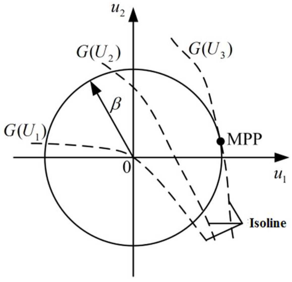
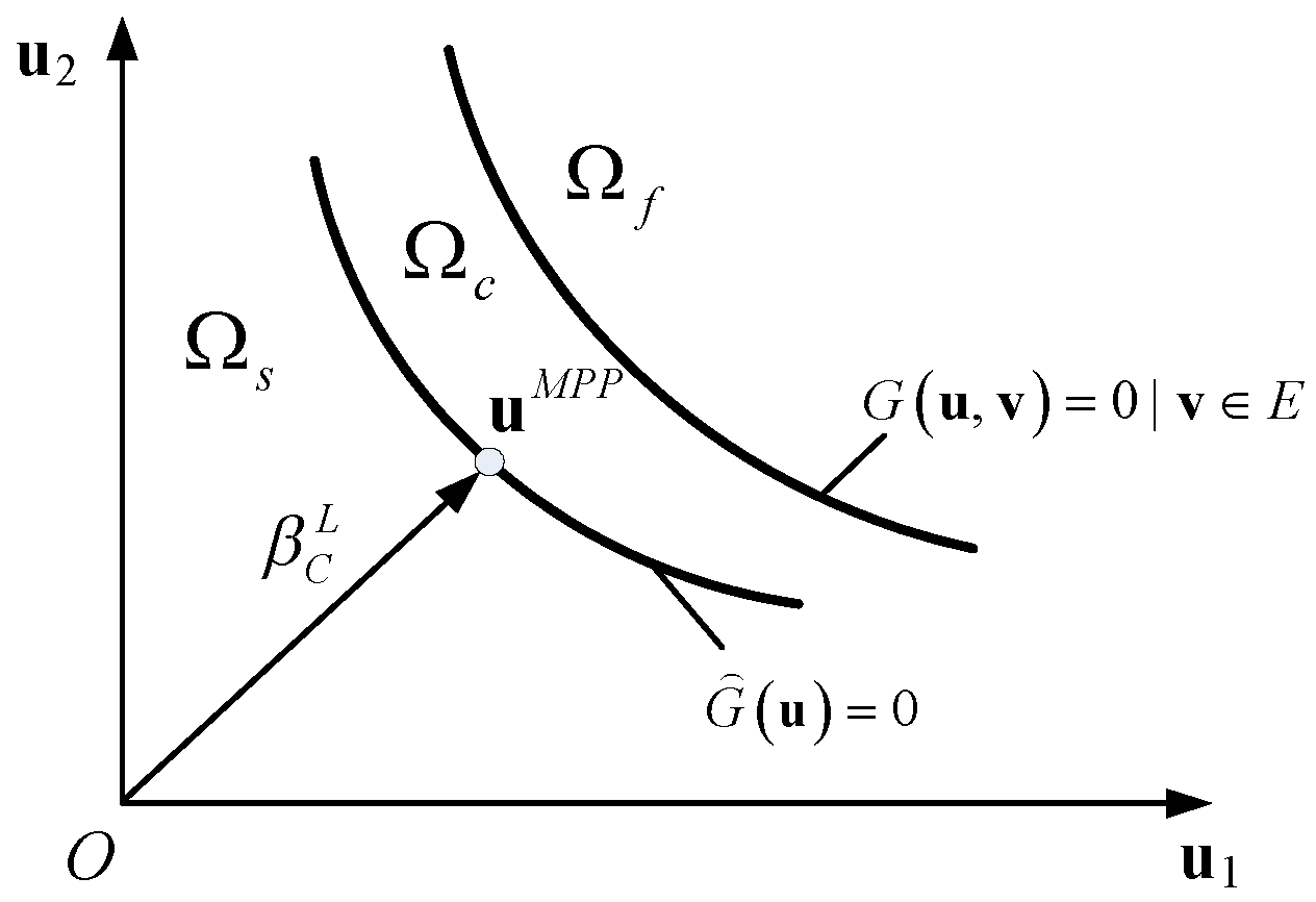
2.2. Performance Measure Approach (PMA) for Reliability Analysis

Performance measure approach (PMA), which is also called inverse reliability analysis method, generally refers to the problem of solving the value of the limit state function under the given reliability index [18]. In the reliability based design optimization, the inverse reliability analysis problem used to evaluate the constraints is usually expressed in the mathematical form as shown in Equation (9).
min   g ( u ) s . t .   u = β
where u is the design variable in the standard normal space, and g(u) is the limit state function in the standard normal space, β represent the specified reliability index. The practical meaning of Equation (9) is to find the point on the specified hypercircular surface that makes the limit state function get the minimum value in the standard normal space. The specified hypercircular takes the coordinate origin of standard normal space as its center and the specified reliability index β as its radius. The point which makes the limit state function minimum is also called most probable point (MPP) of PMA. PMA plays an important role in reliability based design optimization. Through reliability analysis based PMA, the relationship between deterministic constraints and reliability constraints can be established, which provides a strong support for the decoupling of reliability analysis and optimization calculation [6].
The essence of inverse reliability analysis is to solve the optimization problem shown in Equation (9). In order to explain its true meaning more clearly, we will take the two-dimensional (containing two variables) problem as an example. For two-dimensional variable problems, the practical significance of the problem described by Equation (9) can be shown in Figure 1.
It can be seen from the figure that the essence of MPP solved by inverse reliability analysis in standard normal space is the intersection of the specified circle and isoline of state function which has the smallest value and the curve with the smallest value is tangent to the specified circle.
At the same time, when dealing with non-normal aleatory variables, PMA involves fewer nonlinear changes. At the same time, in multidisciplinary system optimization, the PMA method does not need to calculate the specific reliability value and only needs to evaluate the value of limit state function, so the PMA method has high robustness and efficiency for a multidisciplinary system.

3. Materials and Methods

3.1. Reliability Comprehensive Evaluation Index Considering Multisource Uncertainties

When the aleatory uncertainties and epistemic uncertainties are fully considered, the limit state function of the multidisciplinary reliability design optimization model is transformed from the original one which only contains aleatory uncertain design variables and coupling state variables to one which includes both aleatory uncertain variables, epistemic uncertain variables and coupling state variables. Because of the existence of epistemic uncertain design variables, the value of limit state function is no longer a single value (i.e., no longer a single failure surface), but a series of values (i.e., there are a series of failure surface families) between the minimum and maximum values of the limit state function. At this time, the reliability value becomes an interval. In fact, this is also uncertainty, that is, the uncertainties brought by uncertainties.
In order to ensure the high reliability of the design, we propose to use the minimum value of limit state function as the criterion to measure reliability, and the difference of limit state function value to describe the influence of epistemic uncertainties on reliability. The larger the interval difference, the greater the degree of epistemic uncertainties. In fact, the range of the limit state function also directly indicates that designers need to do more experiments on these epistemic variables to improve the reliability of design or obtain more data and knowledge through other channels, reduce the epistemic uncertainty of design parameters, reduce the impact on the limit state function, and then improve reliability of the complex engineering system design.
As shown in Figure 2, the whole standard normal space (U space) is divided by Ω into three parts: safety area (Ωs = {u: min G(u, v, y) > 0|v ∈ E}), critical region (Ωc = {u: min G(u, v, y) = 0|v ∈ E}), and failure region (Ωf = {u: min G(u, v, y) < 0|v ∈ E}). Where u is the standard normal random variables, v is the normalized vector of epistemic variables, and y is the vector of coupling state variable, G(u, v, y) represent the limit state function after space transformation. G(u, v, y) > 0 indicates that it meets the reliability requirements.
The junction of safety area Ωs and critical area Ωc represents a unique spatial curve (surface)   G ( u ) = 0 , which is called “the most probable failure surface”.
The comprehensive evaluation index of multidisciplinary reliability under multisource uncertainty is defined as: in the standard U space, the shortest distance (i.e., the lower limit of interval) from “ the most probable failure surface “ to the coordinate origin is regarded as the reliability evaluation value, and is recorded as β C L (C is comprehensive, which means comprehensive reliability index, L is the lower limit of reliability interval), and the farther the most likely failure surface is from the origin, the smaller the failure probability of limit state function is. In fact, the solution of comprehensive reliability evaluation index can be given by Equation (10):
β C L = min u T u   s . t .   G ( u , v ) = 0
where,
G ( u , v ) = G ( u , v ) s . t .   v i T v i 1 i = 1 , 2 , , n
Equation (10) is used to search for the most probable point (uMPP) of aleatory uncertain variables, and Equation (11) is used to solve the worst point (vWCP) of epistemic uncertain variables. By combining (10) and (11), the MPP can be solved by the multiconstraint optimization problem shown in Equation (12)
Find   ( u , v ) β C L = min u T u   s . t .   G ( u , v ) = 0      v i T v i 1   ( i = 1 , 2 , , n )
Obviously, if epistemic uncertainties do not exist, the comprehensive reliability evaluation index defined in Equation (12) will degenerate to the traditional probability reliability evaluation index. Therefore, the reliability evaluation index proposed in this paper has more general significance.
In addition, the proposed reliability evaluation system can also find the maximum value of the reliability of the limit state function under the influence of the epistemic uncertainties by Equation (13):
β C U = max u T u s . t .   G ( u , v ) = 0
Therefore, the reliability of limit state function under the joint influence of aleatory and epistemic uncertainties is a region, which is expressed as [βL, βU], its difference is recorded as Δβ = βUβL, which directly reflects the influence of the epistemic uncertain design variables on the limit state function. Therefore, the comprehensive evaluation index of multidisciplinary reliability is a kind of generalized reliability evaluation index, which has two meanings: (1) the evaluation index is no longer a single evaluation measure, but a reliability evaluation interval; (2) the difference between the upper and lower limits of the evaluation index directly reflects the influence of epistemic uncertainties on the reliability of limit state function and complex system design.

3.2. Mathematical Model of Reliability with Aleatory and Epistemic Uncertainties

Take Figure 3 as an example. When execute reliability analysis to the constraints of the ith discipline, the mathematical model of which in standard normal space and standard ellipsoid space is as shown in Equation (10):
min   G i N u m ( u s , u i , v s , v i , y i ) s . t .   u s , u i = β t    v i N E T v N E 1 i = 1 , 2 , 3 ; N u m = 1 , 2 , , m ; N E = 1 , 2 , , n
GNumi (us, ui, vs, vi, yi) is the Numth function of reliability constraint of discipline i; us is the system shared aleatory design variables in U space; ui is the aleatory design variables of the ith discipline in U space; vs is the system shared epistemic design variables in V space; vi is the epistemic design variables of the ith discipline in V space; y•i, is the state variables input of discipline i from other disciplines, in which i means the number of disciplines; m represents the number of reliability constraint functions of discipline i, while Num means the number of reliability constraint functions of the ith discipline. According to different types of epistemic uncertainties. It can be divided into NE groups, with each group represented by a single elliptical convex model. The state equation of ith discipline is:
y i = y j i ( u s , u i , v s , v i , y i ) , i , j = 1 , 2 , 3 , i j
This equation can obtain the value of coupling state variables in the following way. This section also takes a complex system consisting of three coupling disciplines as an example (as shown in Figure 4) and explain its MDA process in detail.
us is the shared aleatory design variables of system input, and u1, u2 and u3 are aleatory variables of system input of discipline 1, discipline 2, and discipline 3 respectively; they are local aleatory independent variables. Vs is the shared epistemic design variable of system input, and v1, v2 and v3 are the epistemic variables of system input of discipline 1, discipline 2 and discipline 3 respectively; they are local epistemic independent variables. yij(ij) is the interdisciplinary coupling-state variables, representing the output of discipline i and the input of discipline j. zi(i = 1, 2, 3) represents the output of discipline 1, discipline 2, and discipline 3. In particular, the aleatory variables in this paper refer to variables in line with a certain distribution, while the epistemic variables refer to those with interval uncertainties.
Multidisciplinary analysis under aleatory and epistemic uncertainties is a process that takes full account of system input parameters and calculates the output of system. Because there are different coupling degrees between different disciplines, each discipline output will not only be affected by the discipline input itself, but also by the coupling relationship between disciplines. This means to find each subsystem output, the coupling state variable yij(ij) should be analyzed and evaluated first. Multidisciplinary analysis under aleatory and epistemic uncertainties is similar to that under aleatory uncertainties, including the following steps in detail:
Step 1: List the input-output relationships among each subsystem:
The input-output relationships among discipline 1 is:
{ z 1 = z 1 ( u s , u 1 , v s , v 1 , y 21 , y 31 ) y 12 = y 12 ( u s , u 1 , v s , v 1 , y 21 , y 31 ) y 13 = y 13 ( u s , u 1 , v s , v 1 , y 21 , y 31 )
Step 2: Connect coupling-state variables to establish equations of system analysis.
Take the three-disciplinary coupling system as an example. Its equations of coupling-state system is:
{ y 12 = y 12 ( u s , u 1 , v s , v 1 , y 21 , y 31 ) y 13 = y 13 ( u s , u 1 , v s , v 1 , y 21 , y 31 ) y 21 = y 21 ( u s , u 2 , v s , v 2 , y 12 , y 32 ) y 23 = y 23 ( u s , u 2 , v s , v 2 , y 12 , y 32 ) y 31 = y 31 ( u s , u 3 , v s , v 3 , y 13 , y 23 ) y 32 = y 32 ( u s , u 3 , v s , v 3 , y 13 , y 23 )
Step 3: Select an algorithm and solve it.

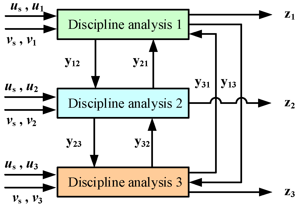
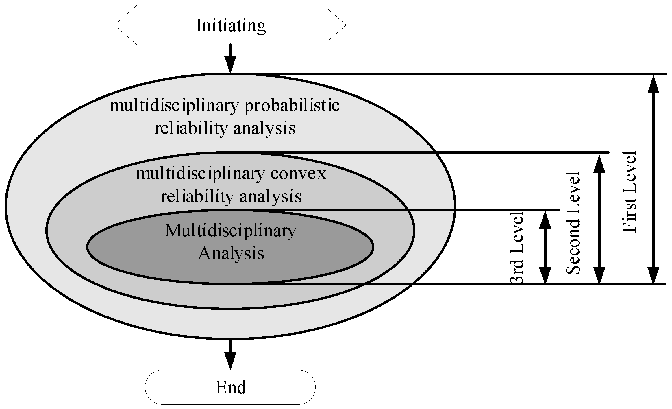
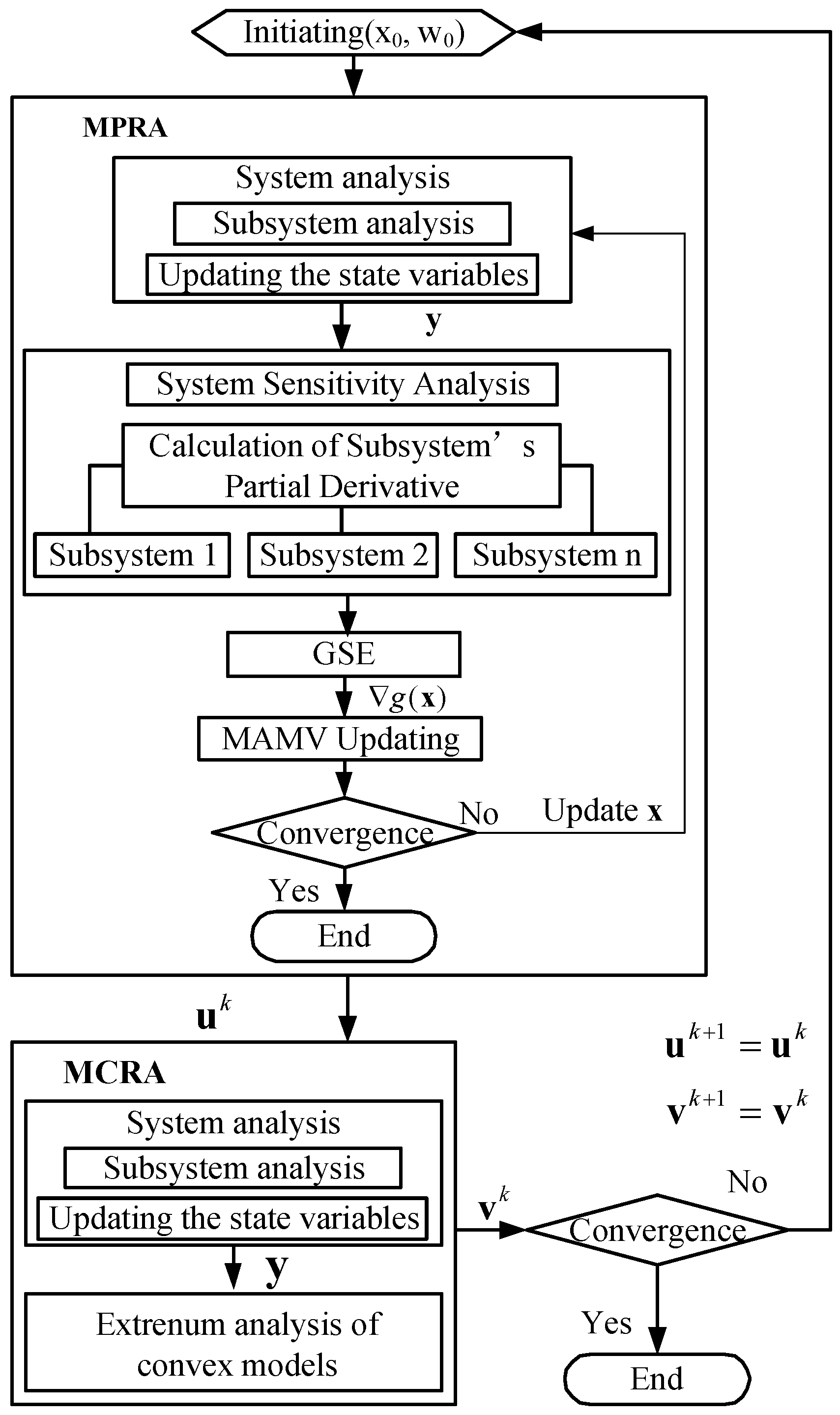
3.3. Decoupling Strategy for Multidisciplinary Reliability Approach

As shown in Figure 4, when both aleatory and epistemic uncertainties are involved, the procedure of MRA will become a nested three-layer loop. The MPRA loop lies in the outer loop, which searches the MPP through calling convex analysis and MDA repeatedly in the standard normal space. The second loop is the MCRA, which aims at finding the minimum of limit state function through calling MDA. The MDA in the inner loop is always invoked repeatedly by MPRA and MCRA, providing the value of coupled limit state function. Obviously, the computational effort of the three-layered procedure may be prohibitive especially for large-scale and coupled multidisciplinary systems.
Therefore, a decoupling strategy for multidisciplinary reliability is proposed to decouple the nested MRA into a sequence of cycles of three modules that are multidisciplinary probabilistic reliability analysis (MPRA), multidisciplinary convex reliability analysis (MCRA) and multidisciplinary analysis (MDA). As a result, a great number of MDA and reliability analyses can be eliminated.
In the MDA module, the values of the coupling state variables are obtained through the coordination relationship among the sub disciplines, and the values of the coupling state variables are used by MCRA and MPRA. So that all the reliability constraints only contain the design variables without coupling state variables.
In convex reliability analysis, Lagrange multiplier method [19] is used to convert constrained optimization problems to unconstrained problems. All epistemic uncertain design variables and Lagrange multiplicator λ are taken derivative based on the differential principle. KKT conditions is used to replace extremum search algorithm. In this way, the calculation efficiency of multidisciplinary convex reliability analysis can be improved.
For multidisciplinary probabilistic reliability analysis. Global sensitivity equations (GSE) [20] based on CSSO strategy are used to provide the prerequisite for parallel subspace sensitivity analysis and provides gradient information for updating the random design variables. Modified advanced mean value (MAMV) [21] method is used to search MPP.
The characteristics of the proposed method are as follows: (1) using PMA to improve the efficiency of reliability analysis from the model itself; (2) decoupling the three-layer nested analysis process; (3) adopting CSSO strategy and executing MDA and global sensitivity analysis to provide reliability analysis with the value and sensitivity information of limit-state functions; (4) adopting KKT conditions to replace the expensive extremum analysis.
When there are only aleatory uncertainties, the method proposed in this paper became a sequential multidisciplinary probabilistic reliability analysis which integrates the CSSO and PMA, as a matter of convenience, we call it SMPRA. When aleatory uncertainties and epistemic uncertainties exist simultaneously, the proposed method is a decoupling based multidisciplinary reliability analysis; we call it MU-DBMRA.
The flowchart of the proposed decoupling strategy is shown in Figure 5. Five steps are involved in this strategy.
Step 1: Set initial values us, ui, vs, vi, k = 1.
Step 2: Multidisciplinary probabilistic reliability analysis.
Step 2.1: Fix epistemic uncertain design variables (characterized by their mean values in first loop), and set loop number k = 1.
Step 2.2: Execute multidisciplinary analysis. Evaluate the value of state variable yk and limit-state functions g(xk).
Step 2.3: Execute system sensitivity analysis. Use GSE method to obtain the gradient of limit-state function x g ( x k ) .
Step 2.4: Convert the aleatory uncertain design variables xk to uk according to the Equation (1), and evaluate the gradient u g ( u k ) of the limit-state function in standard normal space according to the Equation (18):
u g ( u k ) = d g d x k x k u k = x g ( x k ) σ x
where σx are the variance of x.
Step 2.5: Search uMPP by MAMV method.
Step 2.5.1: Calculate the angle between uk and u g ( u k ) according to Equation (19). If γ k ε , execute step 2.7, otherwise step 2.5.2. ε is a small angle for like 0.01°.
γ k = cos 1 u k u g ( u k ) u k u g ( u k )
Step 2.5.2: If g ( u k ) > g ( u k 1 ) , update u according to Equation (20). Otherwise, update u according to Equation (21):
u k + 1 = β t u g ( u k ) u g ( u k )
u k + 1 = β t sin ( γ k ) ( sin ( γ k δ k ) u k u k + sin δ k u g ( u k ) u g ( u k ) )
where βt are the given reliability index. δ k in Equation (21) can be calculated by solving a one-dimensional maximum problem, as shown in Equation (22):
max   g ( u k + 1 ) = g { β t sin ( γ k ) ( sin ( γ k δ k ) u k u k + sin δ k u g ( u k ) u g ( u k ) ) }
Step 2.6: Convergence verification. If ∣uk + 1uk∣ < ε, execute step 2.7. Otherwise, convert the variable uk + 1 to the corresponding variable xk + 1 in original space and then execute step 2.2.
Step 2.7: uMPP = uk, Calculate g(uk), end.
Step 3: Multidisciplinary convex reliability analysis.
Step 3.1: Set aleatory uncertain variables, make u = uMPP.
Step 3.2: Execute multidisciplinary analysis. Calculate the value of state variable yk and limit-state function g(xk).
Step 3.3: Transform constrained optimization problems to unconstrained ones on the basis of Lagrange multiplier method.
Step 3.4: For the newly constructed optimization functions, take partial derivative of the epistemic uncertainties v and λ separately; calculate vmin and vmax,, the corresponding points of the extremum of limit-state functions, by Equation (23).
{ g i λ = 0 g i v i = 0
Step 4: Convergence verification.
Substitute the obtained uk, vkmin and vkmax into limit-state functions. If all multidisciplinary reliability constraints are satisfied and the objective function value converges, execute step 5, or k = k + 1, execute step 2.
Step 5: End.

4. Evaluation and Discussion

In this section, two numerical design examples are used to demonstrate the validity and efficiency of the proposed strategy. The implementation of the algorithm uses the MATLAB programming language.

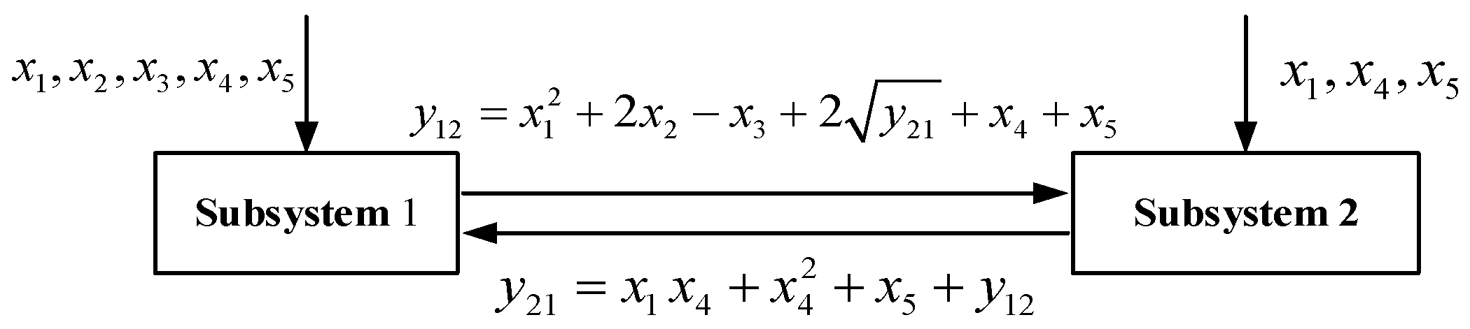
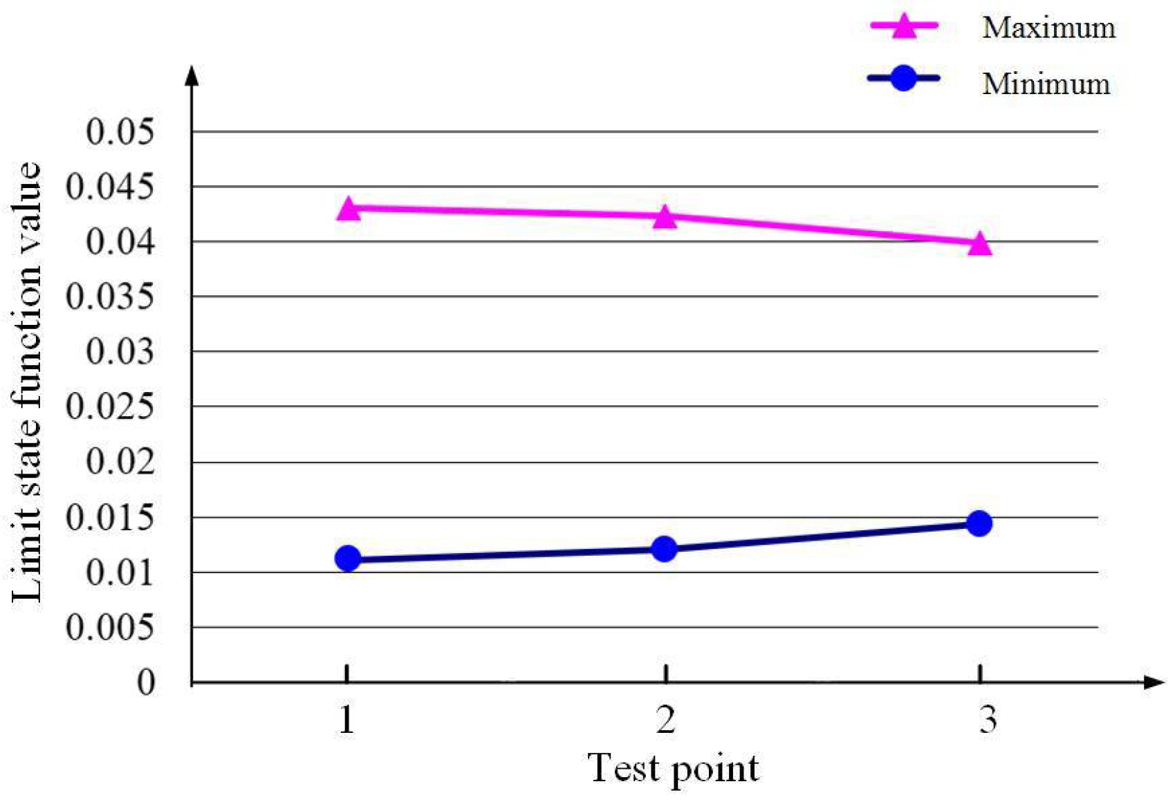
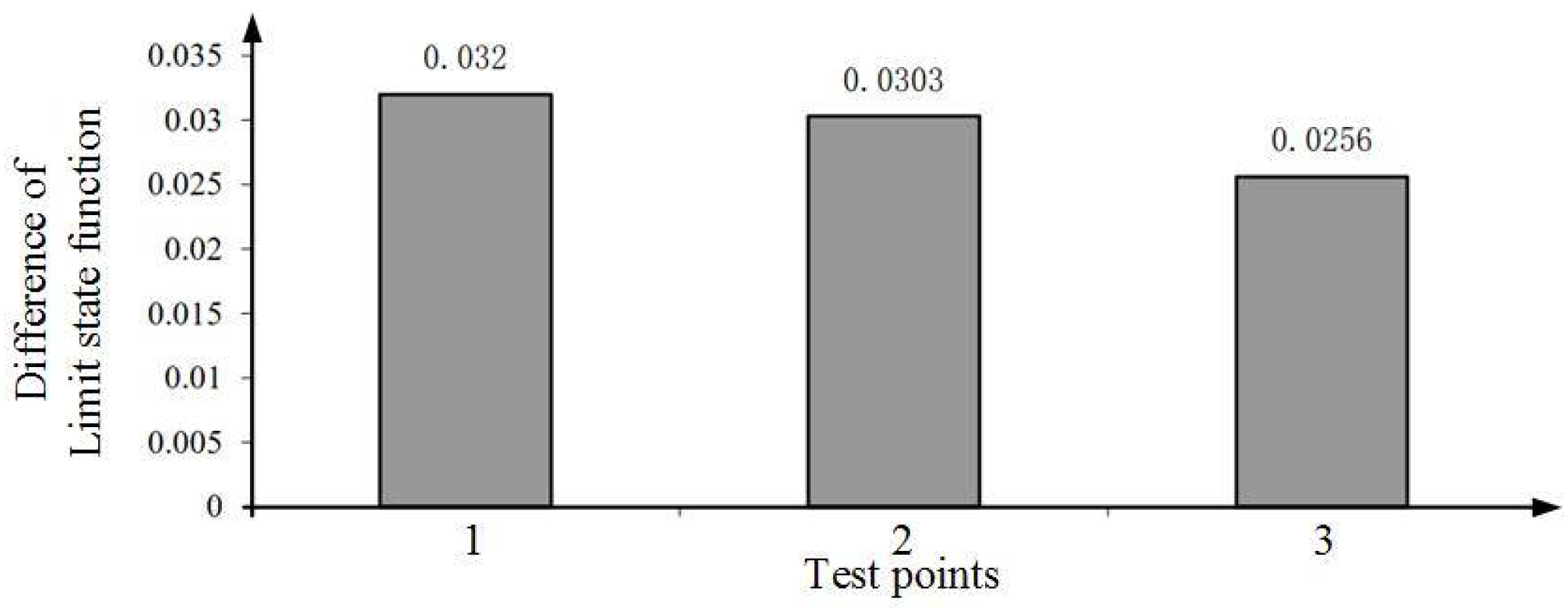
4.1. Numerical Example

As shown in Figure 6, the numerical example [22] consists of three subsystems and five design variables. Where x1, x2, x3 belongs to subsystem 1, subsystem 2 contains three design variables: x1, x4, x5. y12 and y21 are coupling-state variables; g1 and g2 are reliability constraints of subsystem 1 and subsystem 2 respectively.
The functional relationship between the two subsystems is as below:
(1) Subsystem 1:
x 1 = { x 1 , x 2 , x 3 , x 4 , x 5 } , y 1 = { y 12 } , g 1 = { g 1 } y 12 = x 1 2 + 2 x 2 x 3 + 2 y 21 + x 4 + x 5 g 1 = 5 ( x 1 2 + 2 x 2 + 2 x 3 x 4 + x 2 e y 21 ) 1.1 x 5
(2) Subsystem 2:
x 2 = { x 1 , x 4 , x 5 } , y 2 = { y 21 } , g 2 = { g 2 } y 21 = x 1 x 4 + x 4 2 + x 5 + y 12 g 2 = x 1 + x 4 + x 5 ( 0.4 x 1 ) + y 2
In order to verify the effectiveness and computational efficiency of the proposed method, two cases are selected:
Case 1: Suppose that aleatory design variables x = (x1, x2, x3, x4, x5)~N(μx, σx), and the mean value μx = (1, 1, 1, 1, 1), σx = (0.1, 0.1, 0.1, 0.1, 0.1).
Case 2: Suppose that x1, x2 and x3 are design variables with aleatory uncertainty, the mean value μx of x = (x1, x2, x3) equals (1, 1, 1) and the variance σx equals (0.1,0.1,0.1). Similarly, suppose that x4 and x5 are design variables with epistemic uncertainty. Furthermore, in order to further verify the influence of variation range of design parameters with epistemic uncertainty on limit-state functions, three test points are set:
Test point 1: The variation range can be described as below: x E = { x | ( x x ¯ ) T W ( x x ¯ ) 0.04 2 } ; the calibration value is x ¯ = [ x ¯ 4 , x ¯ 5 ] T = [ 1 , 1 ] T and the characteristic matrix is W x = [ 64 0 0 16 ] . Therefore, the conversion relationship of epistemic uncertainties in x-space and in v space is x 4 = v 4 200 + 1 , x 5 = v 5 100 + 1 .
Test point 2: Take the variation ε as 0.02 and the characteristic matrix w11 as 64, w12 as 0, w21 as 0 and w22 as 16, then the conversion relationship of epistemic uncertainties in x space and in v space is: x4 = v4/400 + 1, x5 = v5/200 + 1.
Test point 3: Take the variation ε as 0.04 and the characteristic matrix w11 as 16, w12 as 0, w21 as 0 and w22 as 64, then the conversion relationship of epistemic uncertainties in x space and in v space is: x4 = v4/100 + 1, x5 = v5/400 + 1.
Following multidisciplinary reliability analysis with SMPRA and MU-DBMRA (three test points) methods for the limit-state function g1 respectively, the obtained MPPs, their values and iteration times are shown in Table 1. In order to prove the effectiveness of the algorithm, we chose the method proposed in reference [7] to compare the results in test point 1. The solver of PMA in the contrasting method is sequential quadratic programming (SQP).
From Table 1, it can be seen that the limit-state function value obtained by MCs, MDF + SQP, IDF + SQP and MU-DBMRA methods are all positive, that is, the reliability constraint g1 satisfies the reliability design requirements. The iteration times of MDF + SQP, IDF + SQP and MU-DBMRA are 344, 308 and 258 separately. Mu-DBMRA has the highest efficiency. While, compared with MRA considering only aleatory uncertainties, the iteration times are 232 in SMPRA and 258 in MU-DBMRA respectively for test point 1. Obviously, they have the same magnitude and their calculation efficiency are basically equal. This should be mainly attributed to the following three reasons: (1) decoupling the nested multidisciplinary probabilistic reliability and multidisciplinary convex analysis; (2) adopting Lagrange multiplier method and KKT conditions to replace the expensive function extremum analysis, indicating that this method can keep great calculation effectiveness when dealing with multidisciplinary reliability analysis under aleatory and epistemic uncertainties at the same time.
Theoretically, when design parameters have both aleatory uncertainties and epistemic uncertainties, the limit-state function value should be an interval. As shown in Table 1, 0.0323 ∈ [0.0111, 0.0431], [0.0120, 0.0423], [0.0143, 0.0399], indicating that the single value of limit-state function calculated by SMPRA is in the value range of limit-state function calculated by MU-DBMRA, which, furthermore, verifies the correctness of the proposed method and theory.
From studies of three different test points, the variation tendency of the result for limit-state function analyzed by MU-DBMRA method is shown in Figure 7, and the difference is shown in Figure 8. It is thus evident that as the variation degree of epistemic uncertainties decreases, the maximum of the limit-state function also declines gradually, while the minimum increases gradually. In this way, the difference between the maximum and minimum of the limit-state function tends to diminish gradually. This also suggests that engineering designers need to collect information and data about epistemic uncertainties as much as possible, making it less uncertain and enhancing accuracy of multidisciplinary reliability analysis of the limit-state function. In addition, adopting the minimum of the limit-state function as the standard to test its reliability shows that the result of reliability analysis and design optimization by using MU-DBMRA is safe and reliable design result.

4.2. Speed Reducer

The speed reducer example is a classic problem of MDO [23], containing two subsystems and seven design variables, as shown in Figure 9. Specifically, design variables x1, x2, x3 and constraints g1, g2, g3, g4, g5 belong to gear subsystem; design variables x4, x5, x6, x7 and constraints g6, g7, g8, g9, g10, g11 belong to bearing subsystem.
This design example includes seven design variables: x1 = face width of the gear teeth, x2 = teeth module, x3 = number of pinion teeth, x4 = shaft-length, x5 = shaft length, x6 = shaft diameter, x7 = shaft diameter. Moreover, this design example is composed of 11 constraints (g1~g11) which are related to the bending condition, the compressive stress limitation, the transverse deflection of shafts and the substitute stress conditions. The optimal objective is to minimize the weight of the speed reducer. The constraints of the speed reducer are shown in the Table 2.
The functional relationship between two subsystems is shown as below:
Gear subsystem:
x 1 = { x 1 , x 2 , x 3 } y 21 = { x 4 : x 7 , g 6 : g 11 } g 1 = { g 1 : g 5 }
Bearing subsystem:
x 2 = { x 4 , x 5 , x 6 , x 7 } y 12 = { x 1 , x 2 , x 3 , g 1 : g 5 } g 2 = { g 6 : g 11 }
To verify the effectiveness and calculation efficiency of the proposed method, the set of design variables in the single-stage speed reducer example divided into the following two cases:
Test point 1: Set all the design variable x~N(μx, σx), σx = (0.1, 0.1, 0.1, 0.1, 0.1, 0.1, 0.1) and μx = (3.577, 0.700,17.000, 7.300,7.909,3.427,5.363).
Test point 2: Set the design variable x = (x1, x4, x5, x6, x7)~N(μx, σx), σx = (0.1, 0.1, 0.1, 0.1, 0.1) and μx = (3.577, 7.300, 7.909, 3.427, 5.363). Specifically, x2 and x3 are interval design variables; the vector x ¯ = [ x 2 ¯ , x 3 ¯ ] T = [ 0.700 , 17.000 ] T ; the characristic matrix is that Wx = [4,0, 0,1] with the variation range as x E = { x | ( x x ¯ ) T W ( x x ¯ ) 0.02 2 } .
For test point 1, the reliability index of all limit state functions is set as βt = 3.0. The sequential multidisciplinary reliability analysis method based on MAMV (SMPRA-MAMV) is used to evaluate the reliability. The values of limit state functions g1 to g5, g7, g9 and g11 (which only contains aleatory uncertain variables) and the MPPs are shown in Table 3. It can be seen that the values of g3 and g9 are less than zero, which does not meet the reliability requirements; the values of g1, g2, g4, g5, g7 and g11 limit state functions are greater than zero, which meets the reliability requirements.
For test point 2, the reliability index of all limit state function is set as βt = 3. Obtained MPPs, limit-state function values and iteration times of g7 and g8 through respective multidisciplinary reliability analysis are shown in Table 4 and Table 5. We chose the method proposed in reference [14] to compare the results for g6. The solver of PMA in the contrasting method is sequential quadratic programming (SQP).
From Table 4, it can ve discovered that the values of limit-state function under single aleatory uncertainties and under aleatory and interval uncertainties are all positive, indicating that the constraint condition g6 satisfies the given reliability requirement. Moreover, the value of limit state function under single aleatory uncertainties belongs to the value range of limit state function under random and interval uncertainties, which verifies the correctness of the proposed MU-DBMRA method. In terms of computational efficiency, the proposed MU-DBMRA method needs the least number of iterations when considering the aleatory and interval uncertainties, and its efficiency is 41.7% and 17.8% higher than MDF + SQP and IDF + SQP, respectively, which verifies the correctness and efficiency of the proposed method.
From Table 5, the values of limit-state function under single aleatory uncertainty are positive. In that circumstance, that x = {3.577, 7.300, 7.9000999, 3.427, 5.363} is regarded as a design point for the constraint condition to satisfy the reliability requirment, while for the limit-stage function under aleatory uncertainties and interval uncertainties, its minimum is negative. This is because interval uncertainty changes limit-stage function from a single value to an interval. Only when the interval minimum is positive can the reliaility requirement be satisfied. In this circumstance, that x = {3.577, 7.300, 7.9000999, 3.427, 5.363} cannot be viewed as a design point where the constraint condition satisfies the reliability reqirement. Instead, new design point should be chosen in the proces of RBMDO.

4.3. Discussion

From the above analysis of two examples, the proposd methods need few subsystem analysis times while maintaining accuracy and has a evidently higher calculation efficiency than that of other reliability analysis methods. In addition, the MU-DBMRA method achieves a balance between calculation accuracy and effficiency. In short, the proposed method can handle multidisciplinary reliaility analysis problems under aleatory uncertainty and epistemic uncertainty at a high calculation efficiency with accuracy.
In terms of complexity, both traditional MRA and MU-DBMRA include three modules: probabilistic reliability analysis, convex reliability analysis and multidisciplinary analysis. The complexity of the algorithm can be analyzed from two aspects, one is the complexity of each module, and the other is the time complexity of the whole strategy.
The complexity of each module for MU-DBMRA has been analyzed in Section 3. For probabilistic reliability analysis, the PMA method is used to simplify the model of probabilistic reliability analysis; for convex reliability analysis, KKT conditions is used to replace the expensive extremum analysis. These measures reduce the complexity of the algorithm to some extent.
The time complexity of the whole strategy can be express by the total function evaluation times, which is proportional to the number of iteration steps of the algorithm. As analyzed above, traditional MRA under multisource uncertainties is a three-layer iterative cycle. The total iteration times is the number of iterations of the outermost loop that is MPRA loop. The number of function evaluation is shown in Equation (28).
N f = N MPRA N MDA N ¯ MCRA
where NMPRA is the iteration time of the MPRA loop, NMDA is the iteration time of the MDA loop, and N ¯ MCRA is the average iteration time of MCRA.
The MU-DBMRA method proposed in this paper turns the traditional three-layer nested loop into a serialization process, and its function evaluation times can be expressed by Equation (29).
N f = N Iteration ( N ¯ MPRA + N ¯ MCRA + 2 N MDA )
where NIteration represents the iteration time of the overall large loop, N ¯ MPRA represents the average iteration time of MPRA, and N ¯ MCRA represents the average iterations time of MCRA.
Comparing Equations (28) and (29), we can see that function evaluation times of MU-DBMRA is a quadratic polynomial, while the function evaluation times of traditional MRA is a cubic polynomial. It can be seen from the analysis of the above two cases that the iteration time of the outermost cycles of different methods belongs to the same order of magnitude except Monte Carlo. For the problems with a large number of nonlinear reliability constraints, the complexity of MU-DBMRA is lower than that of traditional MRA.

5. Conclusions

Aiming at the problem of low computational efficiency caused by the three-layer nesting of the MRA, a decoupling strategy for reliability analysis of multidisciplinary system with aleatory and epistemic uncertainties is proposed. This paper integrates the multisource uncertainty quantification based on probability theory and convex set theory. Based on the decoupling principle of multidisciplinary reliability analysis and the idea of serialization, this paper proposes a serialization method of multidisciplinary reliability analysis under aleatory uncertainty and epistemic uncertainty. The three-layer nested loop process is decoupled, and a single loop recursive analysis process is composed of multidisciplinary probabilistic reliability analysis, nonprobabilistic reliability analysis based on convex model and multidisciplinary analysis. In the nonprobabilistic reliability analysis based on convex model, the global sensitivity analysis and KKT condition replacement in the CSSO strategy are integrated to ensure the computation efficiency of the method. The example shows that the method is effective in dealing with the multidisciplinary reliability analysis under aleatory uncertainty and epistemic uncertainty, and has good computational efficiency and accuracy. This method can provide multidisciplinary reliability analysis for RBMDO under aleatory and interval uncertainty, and expand and perfect the RBMDO theoretical system. It is worth noting that the method proposed in this paper also needs to be combined with specific multidisciplinary optimization framework, such as SORA framework, in order to play its specific role, which is our next research focus.
The capability of dealing with uncertainties and the computational efficiency have become the main problems of MRA to be resolved since the current MDO engineering systems are becoming more and more complicated. Therefore, more efforts for future research will focus on: (1) the investigation of probability theory with other mathematical theories (evidence theory, possibility theory, etc.) in quantifying both random and epistemic uncertainties simultaneously, (2) the considerations of correlation of different convex models, and (3) the development of more efficient multidisciplinary reliability analysis methods such as saddlepoint approximation.

Author Contributions

Conceptualization, C.F. and J.L.; methodology, C.F.; software, C.F. and W.X.; validation, C.F. and W.X.; formal analysis, C.F.; investigation, C.F.; resources, J.L.; data curation, C.F. and W.X.; writing—original draft preparation, C.F.; writing—review and editing, C.F. and J.L.; visualization, C.F. and W.X.; supervision, C.F.; project administration, J.L.; funding acquisition, J.L. All authors have read and agreed to the published version of the manuscript.

Funding

This research was funded by National Key Research and Development Program of China, grant number 2018YFB1701703 and National Natural Science Foundation of China, grant number 51475027.

Institutional Review Board Statement

Not applicable.

Informed Consent Statement

Not applicable.

Data Availability Statement

Data sharing is not applicable to this article.

Conflicts of Interest

The authors declare no conflict of interest.

References

  1. Jiang, R.; Sun, T.; Liu, D.; Pan, Z.; Wang, D. Multi-objective reliability-based optimization of control arm using MCS and NSGA-II coupled with entropy weighted GRA. Appl. Sci. 2021, 11, 5825. [Google Scholar] [CrossRef]
  2. Chun, J. Reliability based design optimization of structures using the second-order reliability method and complex-step derivative approximation. Appl. Sci. 2021, 11, 5312. [Google Scholar] [CrossRef]
  3. Faes, M.G.R.; Daub, M.; Marelli, S.; Patelli, E.; Beer, M. Engineering analysis with probability boxes: A review on computational methods. Struct. Saf. 2021, 93, 102092. [Google Scholar] [CrossRef]
  4. Xiang, Z.; Bao, Y.; Tang, Z.; Li, H. Deep reinforcement learning-based sampling method for structural reliability assessment. Reliab. Eng. Syst. Saf. 2020, 199, 106901. [Google Scholar] [CrossRef]
  5. Ghoreishi, S.F.; Imani, M. Bayesian Surrogate Learning for Uncertainty Analysis of Coupled Multidisciplinary Systems. J. Comput. Inf. Sci. Eng. 2021, 21, 041009. [Google Scholar] [CrossRef]
  6. Park, I.; Amarchinta, H.; Grandhi, R. A Bayesian approach for quantification of model uncertainty. Reliab. Eng. Syst. Saf. 2010, 95, 777–785. [Google Scholar] [CrossRef]
  7. Wang, C.; Matthies, H.G. Epistemic uncertainty-based reliability analysis for engineering system with hybrid evidence and fuzzy variables. Comput. Methods Appl. Mech. Eng. 2019, 355, 438–455. [Google Scholar] [CrossRef]
  8. Huang, H.-Z.; He, L.; Liu, Y.; Xiao, N.-C.; Li, Y.-F.; Wang, Z. Possibility and evidence-based reliability analysis and design optimization. Am. J. Eng. Appl. Sci. 2013, 6, 95–136. [Google Scholar] [CrossRef]
  9. Zhang, Z.; Jiang, C.; Wang, G.G.; Han, X. First and second order approximate reliability analysis methods using evidence theory. Reliab. Eng. Syst. Saf. 2015, 137, 40–49. [Google Scholar] [CrossRef]
  10. Li, F.; Liu, J.; Wen, G.; Rong, J. Extending SORA method for reliability-based design optimization using probability and convex set mixed models. Struct. Multidiplinary Optim. 2019, 59, 1163–1179. [Google Scholar] [CrossRef]
  11. Du, L.; Choi, K.K.; Youn, B.D. Inverse possibility analysis method for possibility-based design optimization. AIAA J. 2006, 44, 2682–2690. [Google Scholar] [CrossRef]
  12. Shah, H.; Hosder, S.; Winter, T. Quantification of margins and mixed uncertainties using evidence theory and stochastic expansions. Reliab. Eng. Syst. Saf. 2015, 138, 59–72. [Google Scholar] [CrossRef]
  13. Huang, H.Z.; Zhang, X.D. Design optimization with discrete and continuous variables of aleatory and epistemic uncertainties. J. Mech. Des. 2009, 131, 031006. [Google Scholar] [CrossRef]
  14. Du, X.; Guo, J.; Beeram, H. Sequential optimization and reliability assessment for multidisciplinary systems design. Struct. Multidiplinary Optim. 2008, 35, 117–130. [Google Scholar] [CrossRef]
  15. Meng, D.; Xie, T.; Wu, P.; He, C.; Hu, Z.; Lv, Z. An uncertainty-based design optimization strategy with random and interval variables for multidisciplinary engineering systems. Structures 2021, 32, 997–1004. [Google Scholar] [CrossRef]
  16. Kang, Z.; Luo, Y. Reliability-based Structural Optimization with Probability and Convex Set Hybrid Models. Struct. Multidiplinary Optim. 2010, 42, 165–175. [Google Scholar] [CrossRef]
  17. Rosenblatt, M. Remarks on a multivariate transformation. Ann. Math. Stat. 1952, 3, 470–472. [Google Scholar] [CrossRef]
  18. Youn, B.; Choi, K.; Du, L. Enriched Performance Measure Approach for Reliability-based Design Optimization. AIAA J. 2012, 43, 874–884. [Google Scholar] [CrossRef]
  19. Li, M. Generalized Lagrange multiplier Method and KKT conditions with an application to distributed optimization. IEEE Trans. Circuits Syst. II Express Briefs 2018, 66, 252–256. [Google Scholar] [CrossRef]
  20. Hajela, P.; Bloebaum, C.L.; Sobieszczanski-Sobieski, J. Application of global sensitivity Equations in multidisciplinary aircraft synthesis. J. Aircr. 2012, 27, 12. [Google Scholar] [CrossRef]
  21. Du, X.; Chen, W. An integrated framework for optimization under uncertainty using inverse reliability strategy. J. Des. Manuf. Autom. 2004, 126, 562–570. [Google Scholar] [CrossRef]
  22. Du, X.; Chen, W. Collaborative Reliability Analysis under the Framework of Multidisciplinary Systems Design. Optim. Eng. 2005, 6, 63–84. [Google Scholar] [CrossRef]
  23. Golinski, J. An adaptive optimization system applied to machine synthesis. Mech. Mach. Theory 1973, 8, 419–436. [Google Scholar] [CrossRef]
Figure 1. PMA theory in standard normal space.
Applsci 11 07008 g001
Figure 2. Comprehensive reliability index in u space.
Applsci 11 07008 g002
Figure 3. Multidisciplinary analysis under aleatory and epistemic uncertainties.
Applsci 11 07008 g003
Figure 4. Schematic figure of traditional MRA with the aleatory and epistemic uncertainties.
Applsci 11 07008 g004
Figure 5. The decoupling strategy for multidisciplinary reliability analysis approach.
Applsci 11 07008 g005
Figure 6. The coupling relationship diagram of the numerical example.
Applsci 11 07008 g006
Figure 7. Variation tendency of the limit-state function.
Applsci 11 07008 g007
Figure 8. Difference of maximum and minimum of the limit-state function.
Applsci 11 07008 g008
Figure 9. The coupling relationship diagram of speed reducer.
Applsci 11 07008 g009
Table 1. Reliability analysis results of the numerical example.
Test PointMethodxMPP = {x1, x2, x3, x4, x5}Limi-State Function ValueIteration Times
Case 1SMPRA(1.1726, 1.1726, 1.1726, 1.0017, 1.0017)g1(x) = 0.0323232
Case2:
Test point 1
MU-DBMRA(1.1933, 1.1620, 1.1625, 1.0036, 0.9931)g1(x,v)min = 0.0111258
(1.1937, 1.1623, 1.1617, 0.9964, 1.0069)g1(x,v)max = 0.0431258
MCs(1.2014, 1.1872, 1.1359, 1.0763, 1.0018)g1(x,v)min = 0.0092296,000
(1.2143, 1.1924, 1.1427, 1.0914, 1.0067)g1(x,v)max = 0.0513296,000
MDF + SQP(1.2212, 1.1812, 1.0906, 1.0000, 1.0000)g1(x,v) = 0.0429304
IDF + SQP(1.2209, 1.1816, 1.0951, 1.0000, 1.0000)g1(x,v) = 0.0172276
Case2:
Test point 2
MU-DBMRA(1.1933, 1.1620, 1.1624, 1.0023, 0.9912)g1(x,v)min = 0.0120258
(1.1936, 1.1622, 1.1618, 0.9977, 1.0088)g1(x,v)max = 0.0423258
MCs(1.1879, 1.1564, 1.1607, 1.0008, 0.9847)g1(x,v)min = 0.0021296,000
(1.1952, 1.1693, 1.1684, 1.0042, 1.0106)g1(x,v)max = 0.0657296,000
Case2:
Test point 3
MU-DBMRA(1.1932, 1.1619, 1.1627, 1.0050, 0.9988)g1(x,v)min = 0.0143258
(1.1938, 1.1623, 1.1615, 0.9950, 1.0012)g1(x,v)max = 0.0399258
MCs(1.1884, 1.1579, 1.1631, 1.0021, 0.9864)g1(x,v)min = 0.0074296,000
(1.1804, 1.1672, 1.1616, 1.0032, 1.0094)g1(x,v)max = 0.0362296,000
Table 2. The constraints of the speed reducer.
ConstraintsSpecificationExpression
g 1 Bending stress constraint of gear ( x 1 x 2 2 x 3 ) / 27 .0 1.0 0
g 2 Contact stress constraint of gear ( x 1 x 2 2 x 3 2 ) / 397.5 1.0 0
g 3 Dimensional constraints 1 x 1 / ( 5.0 x 2 ) 1.0 0
g 4 Dimensional constraints 2 12.0 x 2 / x 1 1.0 0
g 5 Dimensional constraints 3 40.0 / ( x 2 x 3 ) 1.0 0
g 6 Small shaft lateral displacement constraint ( x 2 x 3 x 6 4 ) / 1.925 x 4 3 1.0 0
g 7 Large shaft lateral displacement constraint ( x 2 x 3 x 7 4 ) / 1.925 x 5 3 1.0 0
g 8 Minor shaft stress constraint 110 x 6 3 / ( 745 x 4 x 2 x 3 ) 2 + 1.691 × 10 7 1.0 0
g 9 Major shaft stress constraint 85 x 7 3 / ( 745 x 5 x 2 x 3 ) 2 + 1.575 × 10 8 1.0 0
g 10 Dimensional constraints 4 x 4 / ( 1.5 x 6 + 1.9 ) 1.0 0
g 11 Dimensional constraints 5 x 5 / ( 1.1 x 7 + 1.9 ) 1.0 0
Table 3. Probabilistic reliability analysis results of limit state function with aleatory uncertainties.
Limit State Function ValueMPP
x1x2x3x5x7
g1 = 0.49152.99160.675522.99897.80005.2500
g2 = 0.44142.99160.675522.99787.80005.2500
g3 = −0.27522.98010.822323.00007.80005.2500
g4 = 1.69253.01640.676823.00007.80005.2500
g5 = 1.10793.00000.825023.00277.80005.2500
g7 = 11.68883.00000.685422.99817.81705.2160
g9 = −0.06173.00000.749923.00007.80005.1750
g11 = 0.00173.00000.750023.00007.74965.3055
Table 4. The reliability analysis results of g6.
Test PointsMethodValue of FunctonsIteration Times
1SMPRAg6(x) = 6.341124
2MU-DBMRAg6(x,v)min = 1.1816163
g6(x,v)max = 1.3631163
MCsg6(x) = 0.41618,000
MDF + SQPg6(x) = 1.622231
IDF + SQPg6(x) = 1.431192
Table 5. The reliability analysis results of g8.
Test PointsValue of FunctionsIteration Times
1g8(x) = 0.003154
2g8(x,v)min = −0.055188
g8(x,v)max = 0.076188
Publisher’s Note: MDPI stays neutral with regard to jurisdictional claims in published maps and institutional affiliations.

