Partial Discharge Pattern Recognition of Transformers Based on MobileNets Convolutional Neural Network

Abstract
:1. Introduction
2. PD Pattern Recognition Based on MCNN
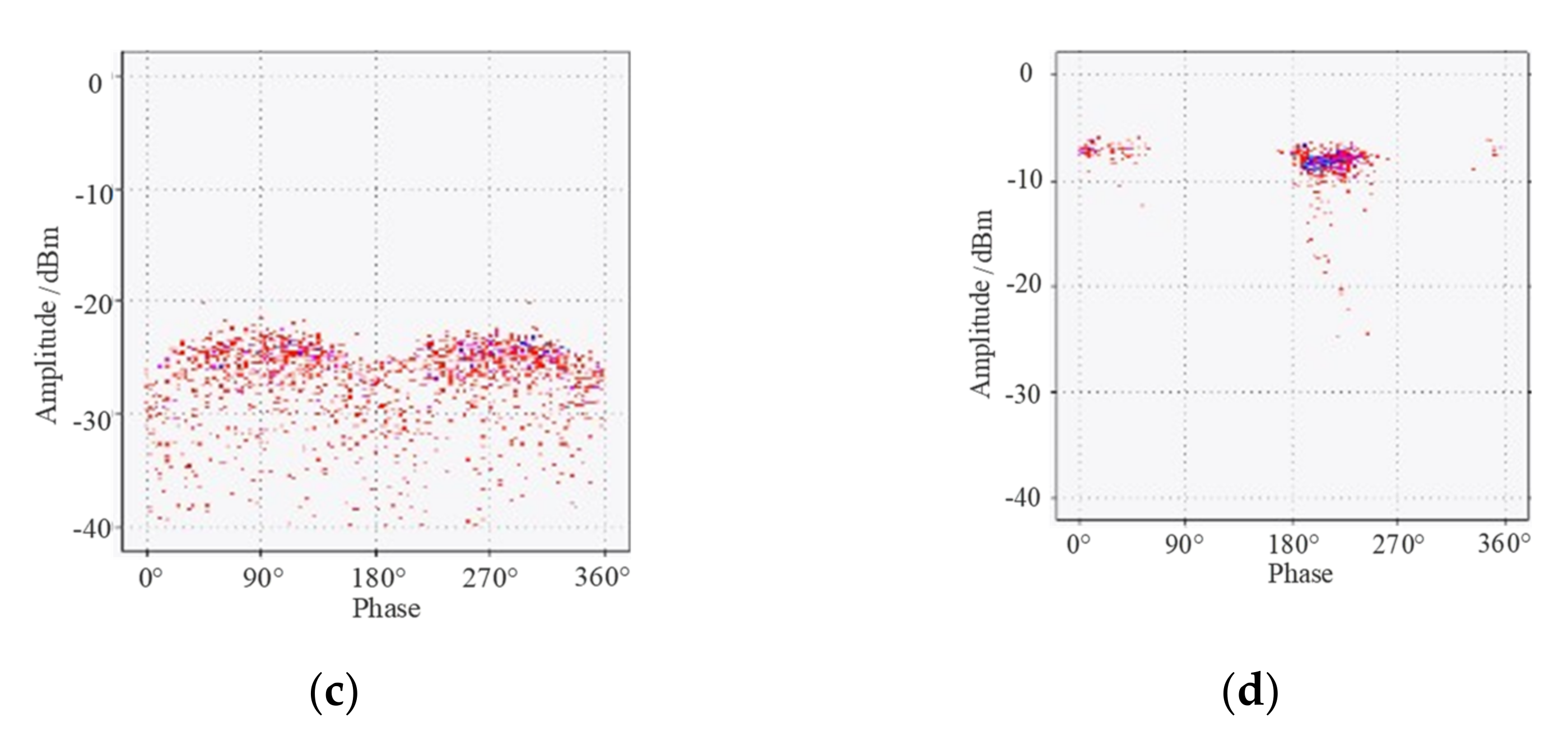
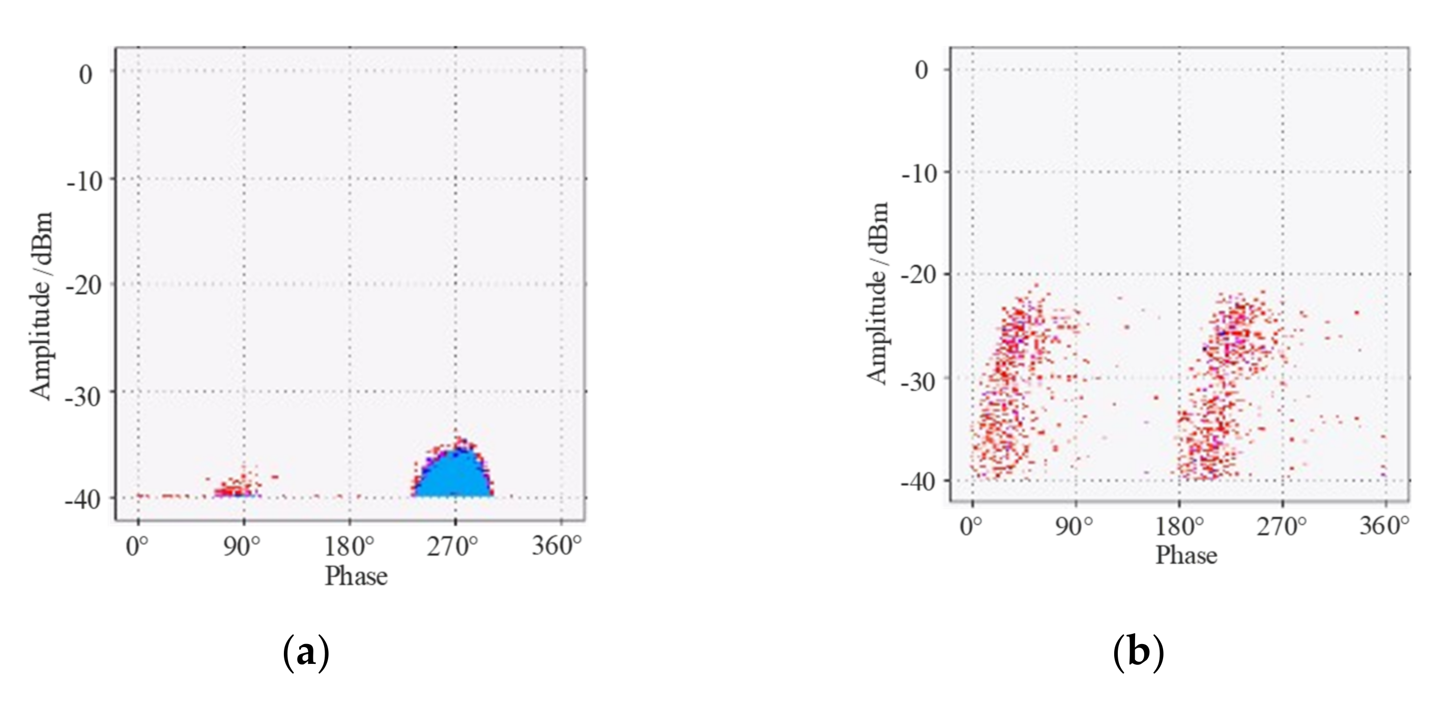
2.1. PD Data Acquisition of Transformer
- (1)
- A PD insulation defect model is selected and connected to the partial discharge test circuit.
- (2)
- The background noise of the laboratory is determined. Before the voltage is applied, the signal detected by the signal acquisition system is the background noise of the PD test environment.
- (3)
- The inception voltage of the PD is determined. The voltage of the regulating transformer is increased uniformly and slowly in steps. When the PD signal is detected by the monitoring instrument, the corresponding voltage is recorded as the initial voltage U1.
- (4)
- The PD data is generated and collected at different voltage supplies. The voltage is continuously increased, and when it is greater than 1.5 times U1, a stable and distinct PD signal series is recorded in the monitoring system. The voltage is then still increased to approximately twice U1. The PD data generated during this process is collected by the UHF sensors. The sensors can record the partial discharge signals of different intensities generated by the partial discharge model at different voltage levels.
- (5)
- Different types of insulation defect models are replaced. After completing the PD test of the current PD insulation defect model, the voltage is slowly lowered and the power is turned off. Different types of insulation defect models are replaced. After completing the PD test for the current PD insulation defect model, the voltage is slowly reduced and the power is turned off. The discharge bar is used to discharge the test circuit, and the insulation defect model is replaced with another one. Then, the experiment steps (2) to (5) are then repeated until all four types of PD data are collected.
2.2. Convolution Neural Network
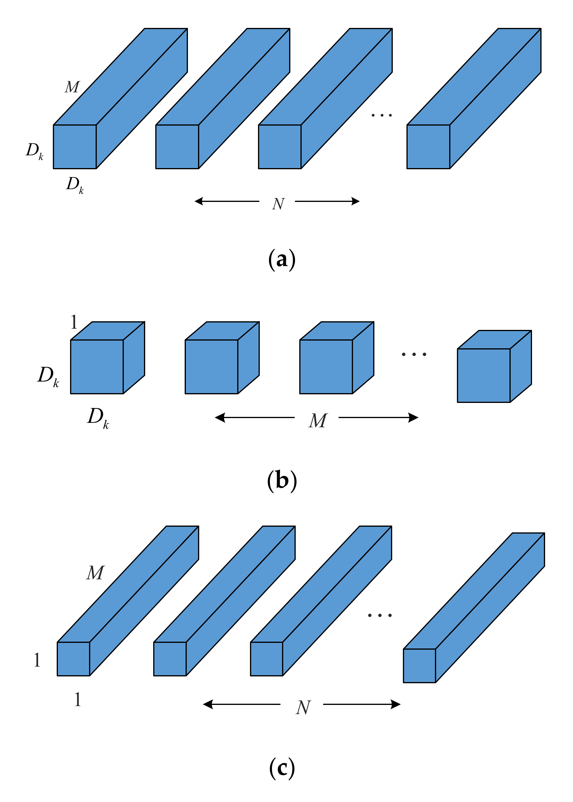
2.3. Mobilenets Convolution Neural Network
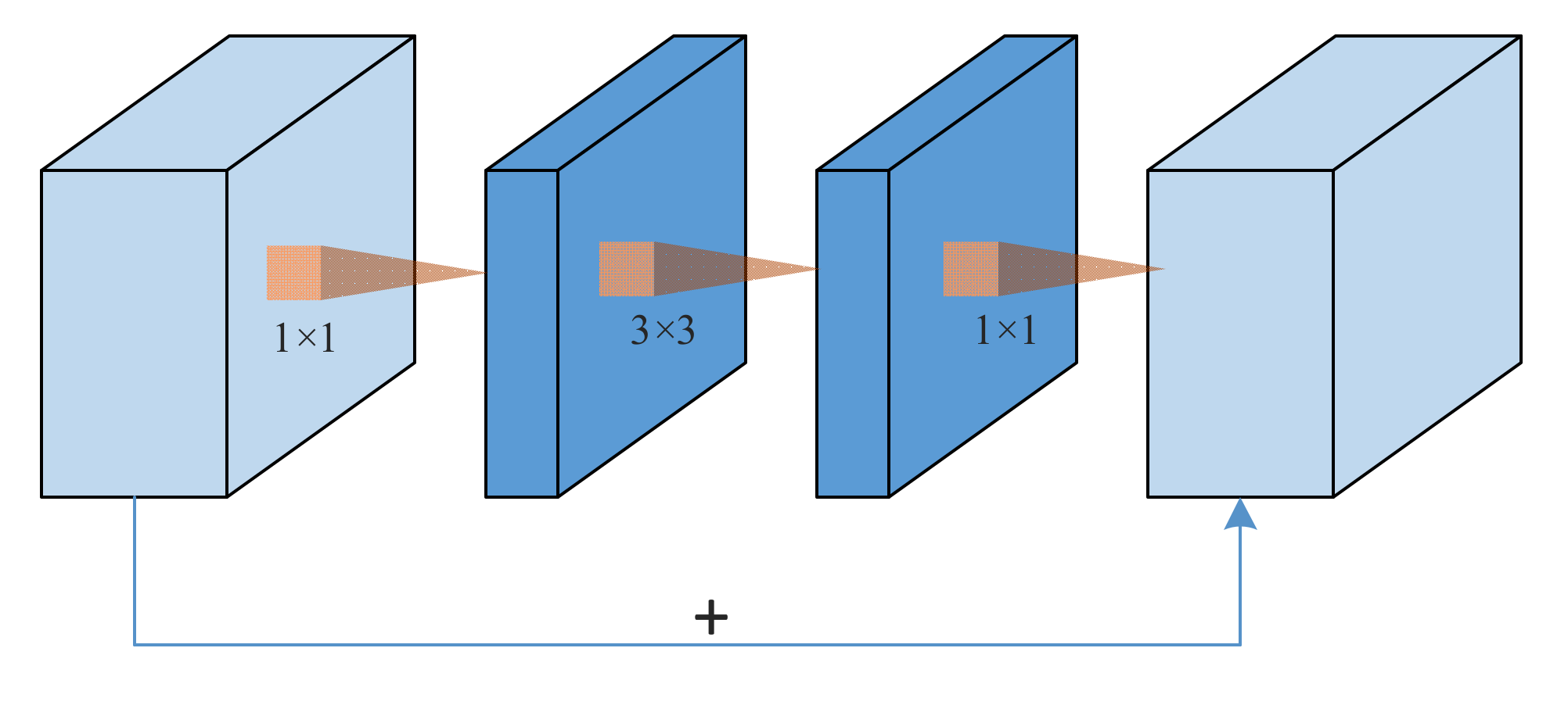
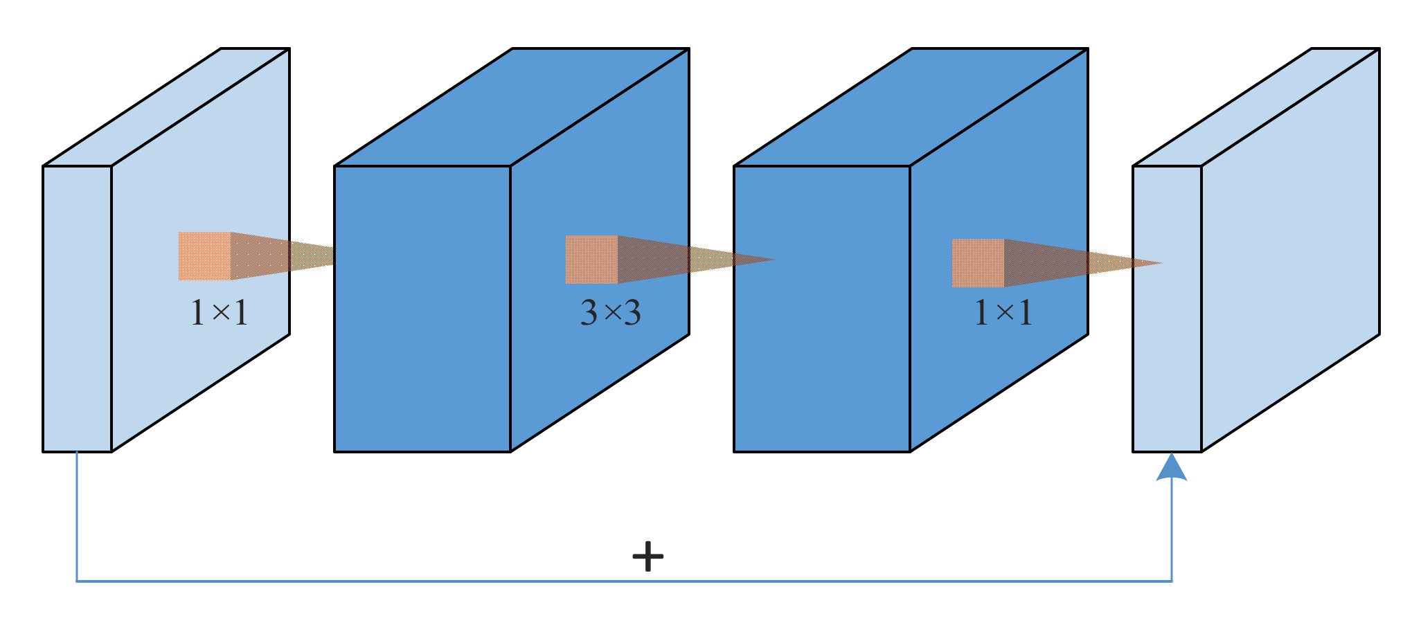
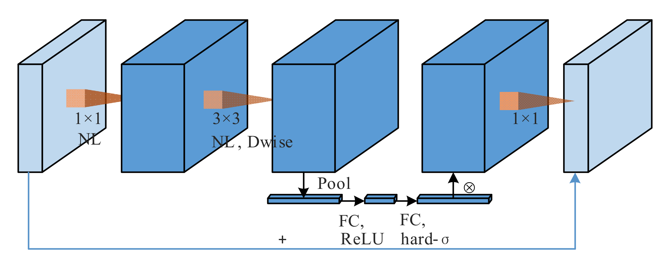
2.4. Lightweight MCNN Block
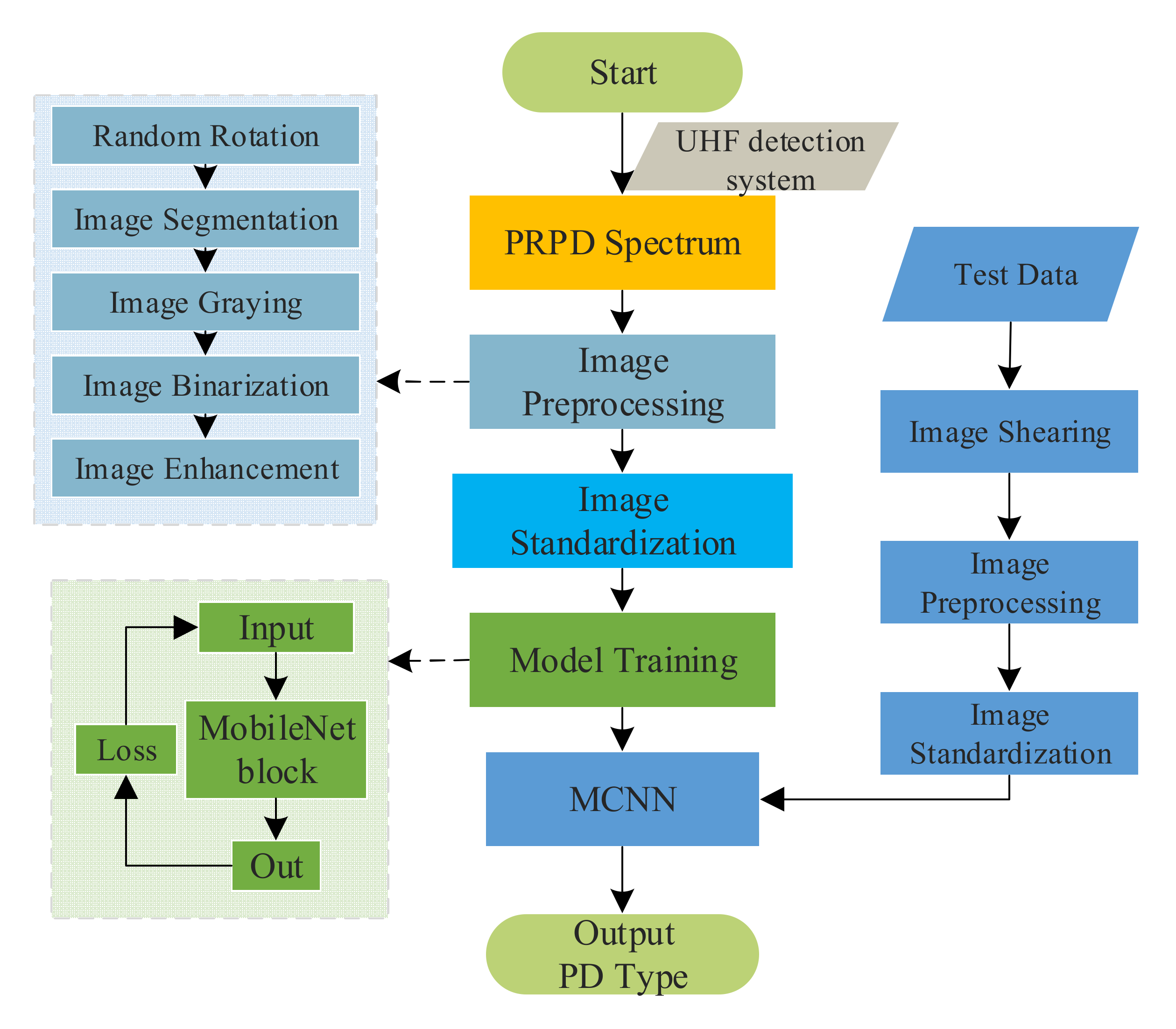
2.5. Training and Testing of MCNN
- (1)
- Data acquisition. According to the data collected by the discharge experiment, the PRPD spectrum is generated, and the collected PD images are randomly divided into the training set and test set, accounting for 80% and 20% of the total samples respectively.
- (2)
- Data preprocessing. Firstly, the PRPD spectrum of PD is randomly allocated to obtain a 224 × 224 × 3 three-channel RGB image, and then the image is flipped randomly and converted into a floating-point tensor with a value between 0~1.
- (3)
- Data enhancement. The sample of the original data is expanded, including random rotation, segmentation, scaling, and other operations. To improve the generalization ability of the model, 20% of the training data is randomly selected by using data enhancement for image generation.
- (4)
- Data standardization. To establish the comparability of the data, the standardized method is used to normalize the input data.
- (5)
- Model training. The loss function used in the training process is the Cross-Entropy Loss, and the optimization algorithm adopted is the Stochastic Gradient Descent. Dropout and Batch Normalization are used to improve the training performance.
- (6)
- Model testing. The trained model is tested on the test set. The purpose of the model testing phase is to verify the generalization ability of the model, and the recognition accuracy of the model to PD data can be obtained.
3. Results
3.1. Recognition Results and Performance Analysis
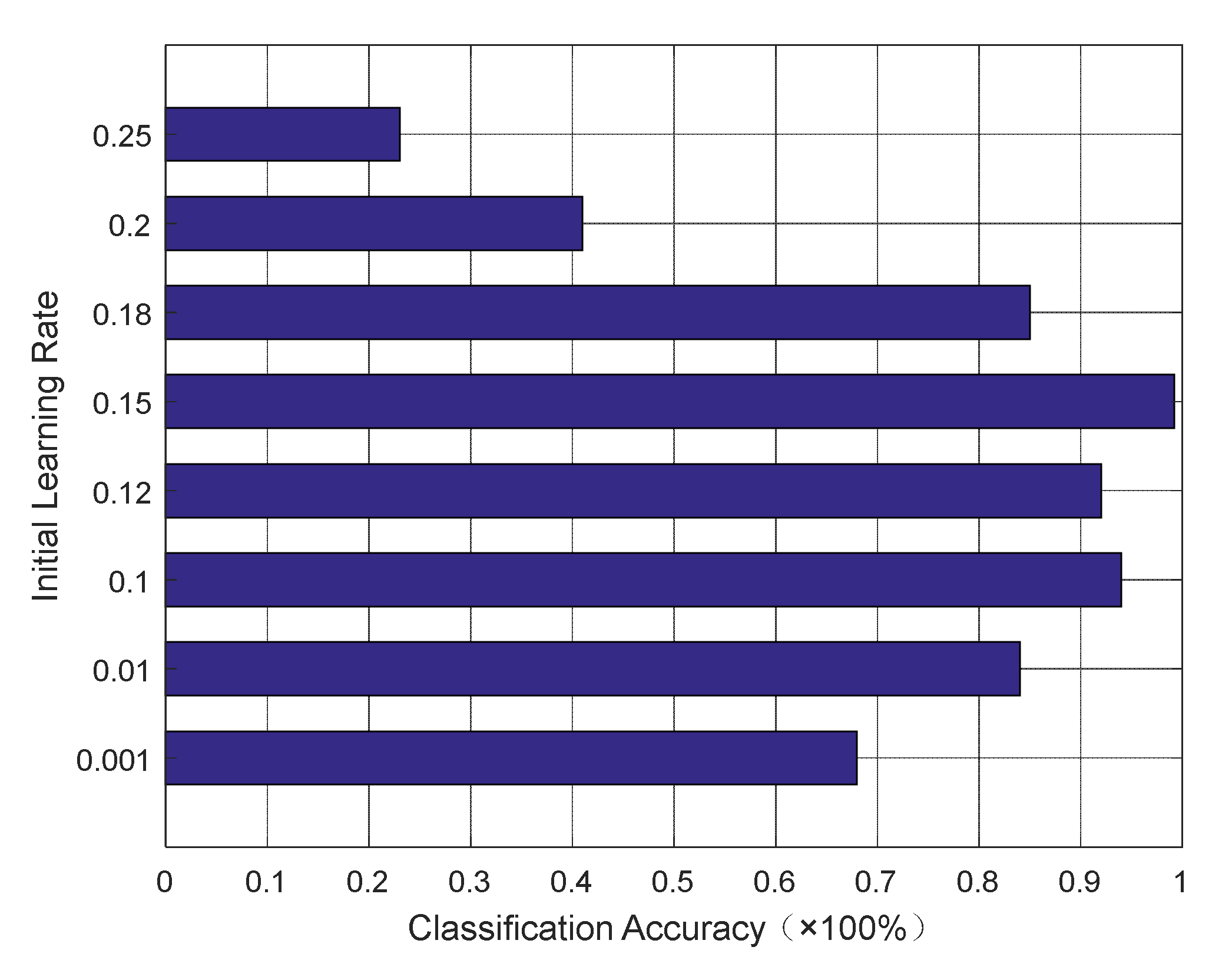
3.1.1. The Effect of Initial Parameters on Network Performance
3.1.2. Classification Performance Comparison of Models
3.1.3. Complexity Analysis of Models
3.1.4. Visual Analysis of MCNN
4. Conclusions
Author Contributions
Funding
Institutional Review Board Statement
Informed Consent Statement
Data Availability Statement
Acknowledgments
Conflicts of Interest
References
- Shang, H.K.; Yuan, J.S.; Wang, Y. Partial discharge pattern recognition in power transformer based on multi-kernel multi-class relevance vector machine. Trans. China Electrotech. Soc. 2014, 29, 221–228. [Google Scholar]
- Zhong, L.P.; Ji, S.C.; Cui, Y.J. Partial discharge characteristics of typical defects in 110 kV transformer and live detection technology. High Volt. Appar. 2015, 51, 15–21. [Google Scholar]
- Li, J.H.; Han, X.T.; Liu, Z.H. Review on partial discharge measurement technology of electrical equipment. High Volt. Eng. 2015, 41, 2583–2601. [Google Scholar]
- Li, J.; Sun, C.X.; Liao, R.J. Study on statistical features used for PD image recognition. In Proceedings of the CSEE, Kunming, China, 13–17 October 2002; Volume 22, pp. 104–107. [Google Scholar]
- Zheng, Z.; Tan, K.X. Partial discharge recognition based on pulse waveform using time domain data compression method. In Proceedings of the 6th International Conference on Properties and Applications of Dielectric Materials, Xi’an, China, 21–26 June 2000. [Google Scholar]
- Gong, Y.P.; Liu, Y.W.; Wu, L.Y. Identification of partial discharge in gas insulated switchgears with fractal theory and support vector machine. Power Syst. Technol. 2011, 35, 135–139. [Google Scholar]
- Ren, X.W.; Xue, L.; Song, Y. The pattern recognition of partial discharge based on fractal characteristics using LS-SVM. Power Syst. Prot. Control. 2011, 39, 143–147. [Google Scholar]
- Ju, F.L.; Zhang, X.X. Multi-scale feature parameters extraction of GIS partial discharge signal with harmonic wavelet packet transform. Trans. China Electrotech. Soc. 2015, 30, 250–257. [Google Scholar]
- Zhou, S.; Jing, L. Pattern recognition of partial discharge based on moment features and probabilistic neural network. Power Syst. Prot. Control. 2016, 44, 98–102. [Google Scholar]
- Schaik, N.V.; Czaszejko, T. Conditions of discharge-free operation of XLPE insulated power cable systems. IEEE Trans. Electr. Insul. 2008, 4, 1120–1130. [Google Scholar] [CrossRef]
- Yin, J.L.; Zhu, Y.L.; Yu, G.Q. Relevance vector ma-chine and its application in transformer fault diagnosis. Electr. Power Autom. Equip. 2012, 32, 130–134. [Google Scholar]
- Zhao, L.; Zhu, Y.L.; Jia, Y.F. Feature extraction for partial discharge grayscale image based on Gray Level Co-occurrence Matrix and Local Binary Pattern. Electr. Meas. Instrum. 2017, 54, 77–82. [Google Scholar]
- Liu, B.; Zheng, J. Partial discharge pattern recognition in power transformers based on convolutional neural networks. High Volt. Appar. 2017, 53, 70–74. [Google Scholar]
- Yuan, F.; Wu, G.J. Partial discharge pattern recognition of high-voltage cables based on convolutional neural network. Electr. Power Autom. Equip. 2018, 289, 130–135. [Google Scholar]
- Wang, X.Q.; Sun, H.; Li, L.G. Application of convolutional neural networks in pattern recognition of partial discharge image. Power Syst. Technol. 2019, 47, 130–135. [Google Scholar]
- Hui, S.; Dai, J.; Sheng, G.; Jiang, X. GIS partial discharge pattern recognition via deep convolutional neural network under complex data source. IEEE Trans. Dielectr. Electr. Insul. 2018, 25, 678–685. [Google Scholar]
- Howard, A.G.; Zhu, M.; Chen, B.; Kalenichenko, D.; Wang, W.; Weyand, T.; Andreetto, M. Hartwig AdamMobileNets: Efficient Convolutional Neural Networks for Mobile Vision Applications. arXiv 2017, arXiv:1704.04861. [Google Scholar]
- Hu, J.; Shen, L.; Albanie, S.; Sun, G.; Wu, E. Squeeze-and-Excitation Networks. arXiv 2017, arXiv:1709.01507. [Google Scholar]
- Howard, A.; Sandler, M.; Chu, G.; Chen, L.C.; Chen, B.; Tan, M.; Wang, W.; Zhu, Y.; Pang, R.; Vasudevan, V.; et al. Searching for MobileNetV3. arXiv 2019, arXiv:1905.02244v5. [Google Scholar]


| Input | Operator | Output |
|---|---|---|
| W × H × N | 1 × 1 conv2d, NL | W × H × t N |
| W × H × t N | 3 × 3 dwise s = s, NL | W/s × H/s × t N |
| W/s × H/s × t N | Linear 1 × 1 conv2d | W/s × H/s × M |
| Layer Num | Input | Operator | Exp Size | Out | SE | NL | s |
|---|---|---|---|---|---|---|---|
| 1 | 2242 × 3 | conv2d, 3 × 3 | - | 16 | - | HS | 2 |
| 2 | 1122 × 16 | Bneck, 3 × 3 | 16 | 16 | √ | RE | 2 |
| 3 | 562 × 16 | Bneck, 3 × 3 | 72 | 24 | - | RE | 2 |
| 4 | 282 × 24 | Bneck, 3 × 3 | 88 | 24 | - | RE | 1 |
| 5 | 282 × 24 | Bneck, 5 × 5 | 96 | 40 | √ | HS | 2 |
| 6 | 142 × 40 | Bneck, 5 × 5 | 240 | 40 | √ | HS | 1 |
| 7 | 142 × 40 | Bneck, 5 × 5 | 240 | 40 | √ | HS | 1 |
| 8 | 142 × 40 | Bneck, 5 × 5 | 120 | 48 | √ | HS | 1 |
| 9 | 142 × 48 | Bneck, 5 × 5 | 144 | 48 | √ | HS | 1 |
| 10 | 142 × 48 | Bneck, 5 × 5 | 288 | 96 | √ | HS | 2 |
| 11 | 72 × 96 | Bneck, 5 × 5 | 576 | 96 | √ | HS | 1 |
| 12 | 72 × 96 | Bneck, 5 × 5 | 576 | 96 | √ | HS | 1 |
| 13 | 72 × 96 | conv2d, 1 × 1 | - | 576 | √ | HS | 1 |
| 14 | 72 × 576 | Pool, 7 × 7 | - | - | - | - | 1 |
| 15 | 12 × 576 | FC, NBN | - | 1280 | - | HS | 1 |
| 16 | 12 × 1280 | FC, NBN | - | k | - | - | 1 |
| Methods | Recognition Accuracy/% | Average Accuracy | |||
|---|---|---|---|---|---|
| Tip Discharge | Surface Discharge | Air-Gap Discharge | Suspended Discharge | ||
| AlexNet | 92.52 | 82.42 | 81.81 | 96.71 | 88.37% |
| ResNet-18 | 94.32 | 88.42 | 90.22 | 100 | 93.24% |
| VGG16 | 93.28 | 88.34 | 86.79 | 97.36 | 91.44% |
| SqueezeNet1.0 | 91.01 | 82.17 | 80.64 | 95.33 | 87.29% |
| DenseNet121 | 100 | 94.37 | 95.54 | 100 | 97.48% |
| MobileNetsV2 | 99.41 | 90.51 | 93.24 | 100 | 95.79% |
| OurModel | 100 | 96.31 | 98.53 | 100 | 98.71% |
| Methods | Parameter/Million | Weight Storage/MB |
|---|---|---|
| AlexNet | 57.02 | 217.51 |
| ResNet-18 | 11.18 | 42.65 |
| VGG16 | 134.29 | 512.28 |
| SqueezeNet1.0 | 0.74 | 2.82 |
| DenseNet121 | 6.96 | 26.55 |
| MobileNetsV2 | 2.23 | 8.51 |
| OurModel | 0.80 | 3.05 |
| Methods | Processing Results | |||
|---|---|---|---|---|
| Original image | 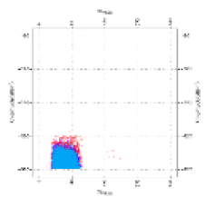 | 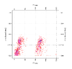 | 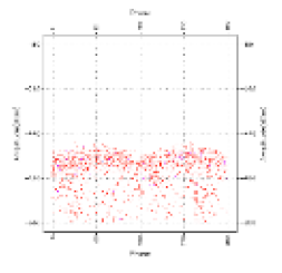 | 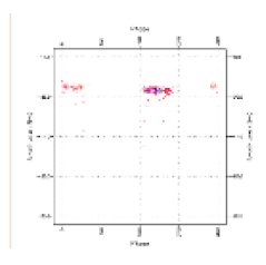 |
| Guided-BP | 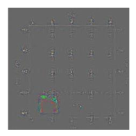 | 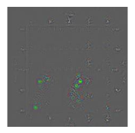 | 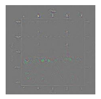 |  |
| CAM | 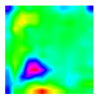 | 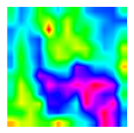 | 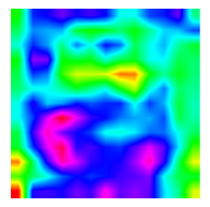 |  |
| Grad-CAM |  | 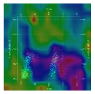 |  | 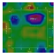 |
| Guided-Grad-CAM | 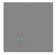 | 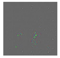 | 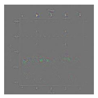 | 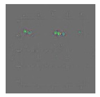 |
Publisher’s Note: MDPI stays neutral with regard to jurisdictional claims in published maps and institutional affiliations. |
© 2021 by the authors. Licensee MDPI, Basel, Switzerland. This article is an open access article distributed under the terms and conditions of the Creative Commons Attribution (CC BY) license (https://creativecommons.org/licenses/by/4.0/).
Share and Cite
Sun, Y.; Ma, S.; Sun, S.; Liu, P.; Zhang, L.; Ouyang, J.; Ni, X. Partial Discharge Pattern Recognition of Transformers Based on MobileNets Convolutional Neural Network. Appl. Sci. 2021, 11, 6984. https://doi.org/10.3390/app11156984
Sun Y, Ma S, Sun S, Liu P, Zhang L, Ouyang J, Ni X. Partial Discharge Pattern Recognition of Transformers Based on MobileNets Convolutional Neural Network. Applied Sciences. 2021; 11(15):6984. https://doi.org/10.3390/app11156984
Chicago/Turabian StyleSun, Yuanyuan, Shuo Ma, Shengya Sun, Ping Liu, Lina Zhang, Jun Ouyang, and Xianfeng Ni. 2021. "Partial Discharge Pattern Recognition of Transformers Based on MobileNets Convolutional Neural Network" Applied Sciences 11, no. 15: 6984. https://doi.org/10.3390/app11156984
APA StyleSun, Y., Ma, S., Sun, S., Liu, P., Zhang, L., Ouyang, J., & Ni, X. (2021). Partial Discharge Pattern Recognition of Transformers Based on MobileNets Convolutional Neural Network. Applied Sciences, 11(15), 6984. https://doi.org/10.3390/app11156984