A Composite Metric Routing Approach for Energy-Efficient Shortest Path Planning on Natural Terrains

Abstract

This paper explores the problem of energy-efficient shortest path planning on off-road, natural, real-life terrain for unmanned ground vehicles (UGVs). We present a greedy path planning algorithm based on a composite metric routing approach that combines the energy consumption and distance of the path. In our work, we consider the Terramechanics between the UGV and the terrain soil to account for the wheel sinkage effect, in addition to the terrain slope and soil deformation limitations in the development of the path planning algorithm. As benchmarks for comparison, we use a recent energy-cost minimization approach, in addition to an ant colony optimization (ACO) implementation. Our results indicate that the proposed composite metric routing approach outperforms the state-of-the-art energy-cost minimization method in terms of the resulting path distance, with a negligible increase in energy consumption. Moreover, our results indicate also that the proposed greedy algorithm strongly outperforms the ACO implementation in terms of the quality of the paths obtained and the algorithm running time. In fact, the running time of our proposed algorithm indicates its suitability for large natural terrain graphs with thousands of nodes and tens of thousands of links.

1. Introduction

Unmanned ground vehicles (UGVs) have been under the scope of research for a long period of time [1]. With the current advancements, it is now possible to integrate UGVs in a broad range of applications, such as autonomous road vehicles [2], information collection and delivery for wireless sensor networks [3], and object detection and face recognition [4]. We are interested in looking at UGV guidance systems for surveillance and exploration purposes on natural uneven rough terrains. Typically, guidance systems take into consideration the problem of path planning on traversable terrain based on predetermined constraints and limitations. Thus, the goal of this work is to propose new methods for planning energy-efficient shortest paths for UGVs crossing over natural terrains. Vehicle path planning can be categorized based on whether offline data are calculated beforehand prior to navigation or real-time sensory input data are being recorded while navigating [5]. We are interested here in the former form of navigation that considers calculating the path offline.

As the power supply for UGVs is limited by the capacity of the carried batteries, it becomes important to consider planning paths with minimum energy consumption, for the purpose of extending the hours of operation [6,7]. As will become evident in the energy cost model discussed in Section II, the vehicle energy consumption along a path depends on the distance of the path, its angle of inclination (i.e., the steepness of the hills being crossed), and the soil trafficability. The soil trafficability is the UGV’s capability to cross over the surface of the terrain without getting stuck due to the wheel sinkage effect related to soil deformation. The wheel sinkage severity is characterized by the contact pressure between the vehicle’s wheels and the terrain surface [8], also known as Terramechanics (vehicle/terrain mechanics). In particular, Terramechanics takes into consideration multiple factors related to the vehicle and the soil sides, known as the main Terramechanics variables [9]. For the vehicle, the main Terramechanics variables are vehicle weight, contact pressure factor, wheels grouser, slippage and friction factors, vehicle ground clearance, bogie factor, engine and transmission factors, and track/tire factor, all of which are used to calculate what is known as the Mobility Index (MI). For the soil, the main Terramechanics variables are the soil cohesion, compactness, homogeneity, sheer stress generated from the vehicle on top of the soil, and humidity percentage. All of the aforementioned factors and variables are used to calculate the Rated Cone Index (RCI) and the Vehicle Cone Index (VCI) factors. These factors are being considered at the core of soil trafficability calculation in this paper, as will be explained later in Section 2.1.

The literature concerned with UGV path planning algorithms is rich and broad; it can be mainly split into two categories. The first is concerned with constructing optimal paths using graph-based path search algorithms such as Dijkstra, Bellman–Ford and/or $A^{*}$ methods, and the second focuses on the use of general-purpose optimization algorithms and heuristics. Examples of studies focusing on graph-based search algorithms can be found in [10,11,12]. The work of [10] explores the Dijkstra algorithm for dynamically solving the problem of energy-efficient path planning for UGVs dropping loads at predefined nodes. However, the study does not take the surface inclination or the soil Terramechanics into consideration. The study in [11] develops a hybrid (offline and online) energy-efficient path planning method for off-road terrain based on a Gaussian Process and an $A^{*}$-like algorithm. A limitation of this work is that only noninclined planer off-road terrains are considered. The work of [12] proposes an energy-efficient path planning and obstacle avoidance algorithm based on an $A^{*}$ algorithm for UGVs on off-road rough terrains. The algorithm employs orthomosaic images and neural networks for path construction. However, the study does not take the soil Terramechanics into consideration.

Examples of studies using general-purpose optimization algorithms and heuristics include [13,14,15]. The study in [13] proposes an energy-aware shortest path optimization algorithm based on a probabilistic roadmap planning method for task-performing UGVs that visit multiple nodes on cattle farms (rough and uneven terrain). The work of [14] considers UGV shortest path planning by employing a chaotic meta-heuristic optimization method based on Q-learning with velocity estimation coupled with Terramechanics. The work of [15] employs a receding horizon path planning algorithm that fragments the main problem into several local path planning problems for UGVs involved in picking-and-delivering operations at multiple nodes. A common aspect of all the above studies is that the investigated problems are formulated as constrained optimization problems that are, in general, hard to solve to exact optimality.

It is worth noting that a bulk of studies in the literature are devoted to path planning and energy management for electric race cars—see, e.g., [16,17,18]. These studies are, in general, concerned with finding optimal trajectories for race cars within their race tracks, often combined with the car velocity control. In particular, the work of [16] proposes a velocity planner optimization algorithm based on multi-parametric sequential quadratic optimization for autonomous electric race cars moving at very high speeds (above 200 km/h). The main inputs for the optimization problem are the energy strategy (power limit), graph-based path planner, and friction estimation. The outputs are the optimal race car velocity and trajectory along this path. Similarly, the study in [17] proposes a three-level semi-offline nonlinear optimization path planning algorithm based on optimal control for autonomous electric race cars lap time minimization. The main inputs for the optimization problem are the thermodynamic variables of the race car, physical constraints such as maximum torque and tires, mathematical constraints such as calculation time, and external constraints such as maximum velocity and obstacles. On the topic of race car lap time minimization, the work of [18] proposes an optimal energy management methodology that achieves the best possible lap time for hybrid electric race cars modeled as a convex optimal control optimization problem. The main inputs for the problem are the vehicle dynamics (mainly the vehicle’s mass and propulsive and drag forces), in addition to physical, operational, and regulatory constraints (such as maximum fuel flow and consumption and turbocharger efficiency). Some other studies have focused on path planning for passenger autonomous vehicles on public roads, such as [19,20]. The work of [19] constructs a cost-function graph model between predefined waypoints, where the road and center lines are represented using parametric cubic spline. The optimal path (lowest cost) and vehicle velocity control are chosen mainly based on static safety (road edges and static obstacles), comfortability (continuity and smoothness of a path), dynamic safety (other vehicles on the road). The study conducted in [20] discussed handling geometry, nonholonomic and dynamics constraints in a human-like and layered fashion. The constructed paths lie in the free space and take in consideration vehicle kinematics and dynamics. The proposed path planning algorithm solves for each constraints individually, starting with global path search, followed by collision checking and path selection, and ending with speed planning. It is worth noting, however, that the above problems have a different mathematical structure and constraints as compared to the UGV path planning problem of this paper. For example, the above studies do not consider natural terrains or soil Terramechanics, but consider aspects of velocity control, thermodynamics and trajectory curvature, which are not present in our problem. Hence, the involved control-theoretic and optimization-theoretic approaches cannot be readily applied to our problem.

Finally, it is worth mentioning that the studies in [6,21,22,23] are also closely related to this paper. In particular, the study in [21] proposes an improved ant colony algorithm for solving the problem of UGV path planning on uneven terrain with soil deformation and slope limitations. However, the study does not consider an explicit energy calculation model and considers only artificial/simulated terrain with a low number of traversal nodes. The study in [22] addresses the problem of finding UGV paths with minimum energy consumption using an $A^{*}$-like algorithm. However, this study does not take the soil Terramechanics into consideration. Moreover, it is based on directly minimizing the energy consumption as a single metric. The study in [6] addresses the problem of UGV shortest path planning on uneven natural terrains, subject to energy consumption constraints. This approach falls under the more general weight-constrained shortest path problem, which is well-known to be NP-hard to solve—see, e.g., [23]. The study in [23] is a preliminary exposition of some of the results presented in this paper. However, and in contrast to this paper, the study in [23] does not consider the soil Terramechanics. This paper adds the soil Terramechanics aspects, effectively resulting in soil trafficability limitations. This paper also adds the ant colony optimization (ACO) [24] implementation to the problem, as well as new results using new natural terrain graphs.

We highlight the contributions of this paper as follows.

• We propose a new greedy (Dijkstra-like) path planning algorithm for UGVs on irregular natural real-life terrains. The algorithm is based on a composite routing metric that combines the distance and energy consumption of the path.
• We consider the vehicle–soil contact Terramechanics in our algorithm, which involves the vehicle structure information and soil composition data. The algorithm also takes realistic soil and slope limitations, UGV power limitations and air humidity into account.
• Our numerical results indicate that the proposed composite metric performs better than the direct energy consumption metric in terms of reducing the overall constructed path distance, with a minimal increment in the energy consumption. Thus, our proposed approsach strikes a better balance between the path distance and energy consumption. Additionally, it is verified that the proposed greedy algorithm strongly outperforms the ACO implementation in terms of both the path distance and consumed energy, and algorithm running time.
• Our numerical running time results demonstrate that our algorithm is well-suited for sizable natural terrain graphs with thousands of nodes and tens of thousands of links.

The remainder of paper is organized as follows. Section 2 presents the needed preliminary information, such as soil trafficability, and the employed energy model. In Section 3, we present the energy-efficient shortest path planning algorithm based on the composite metric routing approach. Section 4 lays out the simulations setup and illustrates the simulation results and discussion. Finally, Section 5 concludes the paper.

2. Preliminaries

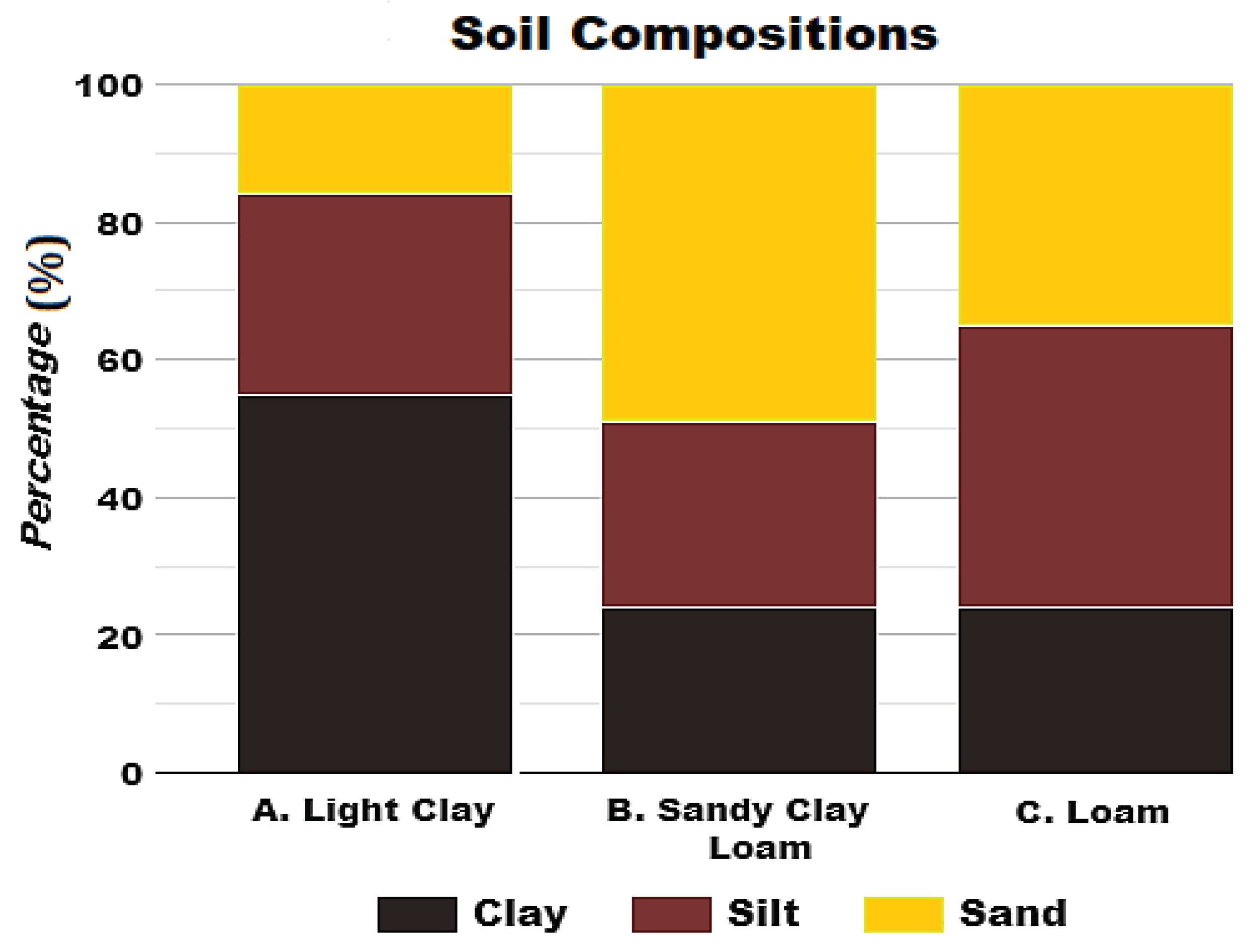
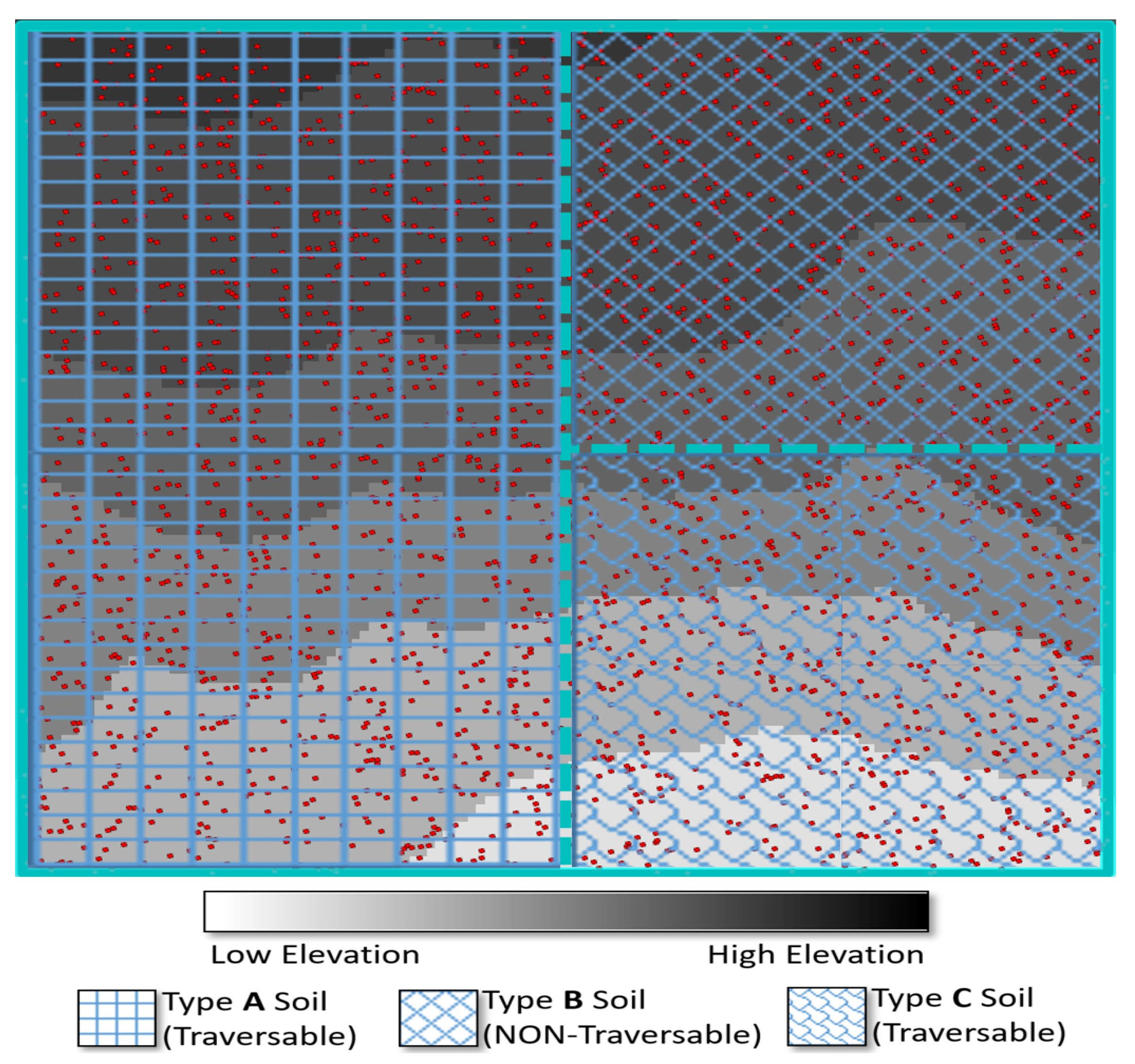
2.1. Soil Trafficability

An important aspect of this paper addresses the ability of the UGV to pass over the different types of soil compositions found in the terrain under consideration. One of the most famous soil categorization systems is based on the Unified Soil Classification System (USCS), which is issued by the United States Department of Agriculture and detailed in [25]. In general, there are three types of soil that act as primary classifiers for the USCS, namely silt, clay, and sand. The real-life terrain considered for UGV routing in this work has the soil decomposition that is described in Figure 1. Our discussion here focuses on the capability of the UGV to move over the soil types analyzed in Figure 1. This is quantified using the RCI and VCI measures for the soil and vehicle, respectively. The RCI is an index of the soil shear strength that includes consideration of the sensitivity of soil to strength losses under vehicular traffic [9]. In particular, and following the methodology in [21,26] for computing the RCI values for different soils and air humidity percentages, Figure 2 depicts the RCI values for soil types A, B and C (of Figure 1) for a wide range of humidity changes in the atmosphere. On the other hand, the VCI is a vehicle-specific metric [9] and is calculated using the MI factor, which depends on the vehicle specifications and the number of repetitive vehicle crossings over the same soil spot. The soil trafficability is evaluated by the following comparison

$$\left\{\begin{array}{cc}\mathrm{Soil}\mathrm{is}\mathrm{Traversible}\hfill & VCI<RCI\hfill \\ \mathrm{Soil}\mathrm{is}\mathrm{NON}-\mathrm{Traversible}\hfill & VCI⩾RCI.\hfill \end{array}\right.$$

(1)

The soil trafficability is calculated based on the type of soil on which the nodes are placed in the simulated real-life terrain model. A more detailed look over the soil and vehicle information for the terrain utilized in this work is given in Section 4.2.

2.2. Terrain Model Generation

We resort to the use of the publicly available digital elevation models (DEMs) to prepare the simulation setup for the real-life terrains under study. To this end, we modeled the natural terrain as a graph. Nodes are scattered in the area of consideration, where some node pairs are connected via traversable links. A UGV will be moving from its source node, traversing a sequence of links until it reaches its desired target node. Similar to [22], a visual representation of a sample terrain graph is given in Figure 3, where each node is connected to eight other neighboring nodes via links. The details on the distribution and allocation of nodes and links will be elaborated on later in Section 4.2. Each link’s energy cost, distance cost, and soil trafficability will play an important role in the developed energy-efficient shortest path routing algorithm. In what follows, we describe the calculation of the used link metrics: distance and energy cost.

2.3. Distance and Energy-Cost Calculations

Let n be a general node in the terrain graph, and let $x_n$, $y_n$, and $z_n$ denote its coordinates in space, respectively. The three-dimensional (3D) Euclidean distance between two nodes m and n can be calculated as follows

$$d(m,n)=\sqrt{{(x_m-x_n)}^2+{(y_m-y_n)}^2+{(z_m-z_n)}^2}.$$

(2)

Considering the distances $d(m,n)$ as link labels in a shortest path algorithm would result in the path with shortest physical distance from source to destination. However, our objective here is to also produce an energy-efficient route to comply with the UGV’s power limitations. Thus, for energy-cost calculations, we employ the model from [27].

The angle of inclination for any two neighboring nodes on the terrain can be expressed as follows

$$\varphi (m,n)=ta{n}^{-1}\left(\frac{z_n-z_m}{\sqrt{{(x_m-x_n)}^2+{(y_m-y_n)}^2}}\right).$$

(3)

It is easy to see that a positive angle of $\varphi (m,n)$ reflects that the UGV is going up a hill, while a negative angle means that it is going down a hill.

The inclusion of the energy cost into the physical model does not only serve the purpose of creating energy-efficient paths, but it also captures the case when it is unfeasible for the UGV to climb up a steep hill based on the angle of inclination and the available power. Our work assumes that the UGV is moving at a fixed velocity v. Furthermore, we assume that the only two forces exerted on the UGV are gravity and the wheel-terrain friction. The combination of these two forces can be expressed as $mg(\mu cos\vartheta +sin\vartheta )$, where m is the mass of the UGV, g is the acceleration of gravity, and $\mu$ is the friction coefficient. It was reported experimentally in [28] that this methodology is limited to a small error margin of $1\%$ for small slopes. It can be easily shown that the energy cost for a link between two nodes is $mgd(m,n)\left(\mu cos\varphi (m,n)+sin\varphi (m,n)\right)$.

Now, we discuss the terrain untrafficability due to power limitations while climbing steep hills. We start with quantifying the power available in-hand for the UGV by defining the vehicle’s output force as $F_{UGV}=P_{max}/v$, where $P_{max}$ is the maximum output power by the UGV. We conclude that, based on the used physical model, the maximum angle of inclination for a hill that the UGV is able to move forward up within its capabilities is

$${\varphi }_{UGV}={sin}^{-1}\left(\frac{F_{UGV}}{mg\sqrt{{\mu }^2+1}}\right)-{tan}^{-1}\left(\mu \right).$$

(4)

This concept can be expanded to any terrain with a slope. It should be stated that wheels’ traction on soil can be lost, especially at great inclination angles. Thus, the static friction ${\mu }_{st}$ for the UGV is considered. The traction-loss cases can occur when the angle of inclination is larger than ${\mu }_{st}$ [27]. This angle can be obtained as

$${\varphi }_{st}={tan}^{-1}({\mu }_{st}-\mu ).$$

(5)

This further imposes restrictions on he UGV’s capability of crossing steep inclined hills. Therefore, we can define ${\varphi }_{up}$ as the dead angle, above which the UGV is unable to pass, either due to power limitations or loss of traction. In particular,

$${\varphi }_{up}=min({\varphi }_{UGV},{\varphi }_{st}).$$

(6)

In other cases, when the UGV is heading down a steep hill, the resultant external force exerted on the UGV is zero. This only occurs when the UGV’s degree of inclination is smaller than ${\varphi }_{down}$, which is defined as the critical breaking angle. It can be shown that [22]

$${\varphi }_{down}=-{tan}^{-1}\left(\mu \right).$$

(7)

Subsequently, if the UGV’s angle of inclination is ${\varphi }_{UGV}<{\varphi }_{down}$, the UGV is moving under its own weight because of the gravitational force vector alignment in the same direction of vehicle movement. Therefore, the energy cost is negative. It should be noted that the only type of energy required under such scenario is for braking to maintain a constant UGV velocity. Additionally, there is energy needed for turning the vehicle’s wheels. However, following [27,29], we assume these forces to be negligible. Henceforth, the energy cost is assumed to be zero if the angle of inclination is less than ${\varphi }_{down}$ to make sure that all traversal links in the terrain graph are given non-negative energy-cost values. We can now present the complete model that takes into consideration the movement forces and vehicle limitations to calculate the energy cost $e(m,n)$ per link $(m,n)$ as follows

$$e(m,n)=\left\{\begin{array}{cc}0\hfill & \varphi (m,n)<{\varphi }_{down}\hfill \\ mgd(m,n)(\mu cos\varphi (m,n)+sin\varphi (m,n))\hfill & {\varphi }_{down}\le \varphi (m,n)\le {\varphi }_{up}\hfill \\ \infty \hfill & \varphi (m,n)>{\varphi }_{up}OR VCI(m,n)⩾RCI(m,n).\hfill \end{array}\right.$$

(8)

3. Composite Metric Routing Approach

It is worth noting that the distance metric of (2) can be used by a shortest path algorithm, e.g., Dijkstra or Bellman–Ford, to find the path from source to destination with minimum physical distance/length. On the other hand, the energy-cost metric of (8) can be also used by a shortest path algorithm to find the path from source to destination with minimum required energy consumption, with no explicit consideration to the distance of the path. To void the NP-hardness of finding the path with shortest distance subject to constraints on the energy consumption, we propose the following composite routing metric that combines the path distance and energy consumption in a multiplicative fashion.

3.1. Composite Metric

Let $D\left(L\right)$ represent the total distance of any path L as follows

$$D\left(L\right)=\sum _{\forall (m,n)\in L}d(m,n),$$

(9)

where $d(m,n)$ is the distance of link $(m,n)$ as provided by (2). Additionally, let $E\left(L\right)$ represent the total energy cost of traversing path L. Hence,

$$E\left(L\right)=\sum _{\forall (m,n)\in L}e(m,n),$$

(10)

where $e(m,n)$ is the energy cost of link $(m,n)$ as provided by (8). Our proposed composite metric $M\left(L\right)$ for path construction is defined as follows

$$M\left(L\right)=D\left(L\right)\times E\left(L\right).$$

(11)

The main idea here is to use a routing metric that combines both aspects of path distance and energy consumption. Thereby, we are hoping to be able to find routing paths that strike a better balance between the distance and energy consumption, as opposed to minimizing the energy consumption alone, or minimizing the distance alone. It is worth noticing that shortest path algorithms, such as Dijkstra or Bellman–Ford, are not guaranteed to converge unless the used routing metric is monotone [30,31]. Moreover, convergence to an optimal path requires the routing metric to be also isotonic. In particular, monotonicity of a routing metric implies that the overall path metric does not improve when it is extended by a new link, while isotonicity of a routing metric implies that the weight-relationship between two paths remains unchanged if both paths are extended by a common link. It has been shown in [23] that the composite metric given by (11) is indeed monotone. Furthermore, it has been also shown in [23] that the composite metric (11) is not isotonic. The latter fact implies that convergence to an optimal path is not guaranteed if the metric (11) is minimized via a shortest path algorithm. However, we observed that an optimal path was indeed found in the vast majority of our numerical experiments, when the Dijkstra shortest path algorithm was used.

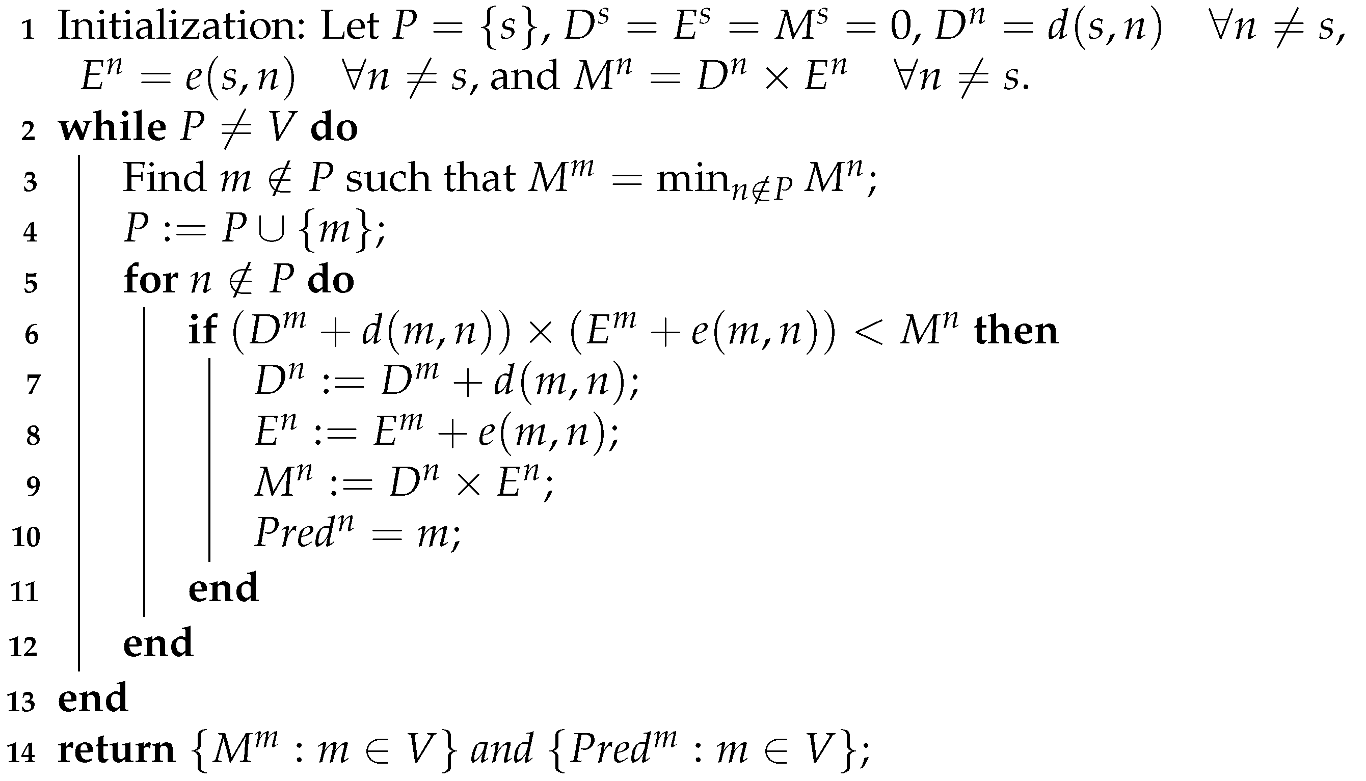
3.2. The Proposed Greedy Implementation

We define the following terms before describing the proposed greedy algorithm. The terrain is modeled as a graph $G=(V,A)$, where V is the set of nodes/vertices and A is the set of links/arcs. The distance of any link $(m,n)\in A$ is given by $d(m,n)$ as in (2). The energy cost of any link $(m,n)\in A$ is given by $e(m,n)$ as in (8). The distance and energy costs between any node and itself is zero, i.e., $d(m,m)=e(m,m)=0$. It is also noted that if $(m,n)\notin A$, then $d(m,n)=e(m,n)=\infty$. Moreover, the following definitions are in order.

• $s,f$ Source and final (or finish) nodes of the required path, respectively;
• $D^n$ Distance of best path from the source node s to node n;
• $E^n$ energy cost of best path from the source node s to node n;
• $M^n$Composite Metric of best path from the source node s to node n, i.e., $M^n=D^n\times E^n$;
• P Set of nodes for which the best path from s is known;
• $Pre{d}^n$ Predecessor of node n on the best path from the source node s.

Now, we can state the proposed algorithm as shown in Algorithm 1.

Algorithm 1:Composite Metric Greedy Implementation

Note that after the algorithm terminates, $M^f$ will be equal to the composite metric of the selected path from source s to final node f. Moreover, the selected path itself can be constructed by tracing $Pre{d}^n$ backwards. In other words, the selected path can be constructed backwards as follows: $\{n_1=f,n_2=Pre{d}^{n_1},n_3=Pre{d}^{n_2},\dots ,s\}$. It can be easily seen that the computational complexity of composite metric greedy implementation is $O\left(\right|V{|}^2)$. In fact, the above greedy algorithm is a modification to the Dijkstra shortest path algorithm, where the composite metric is used instead of the link distance metric.

The details of our proposed Algorithm 1 and its simulation context can be described as follows. The simulation starts with loading offline data into the algorithm. These data are composed of the elevation of the nodes, distances between neighboring nodes, and soil information for each node on the terrain under study, in addition to the air humidity and vehicle information. Consequently, we are also able at this point to calculate the energy cost per link (8) offline, and feed this information to the algorithm. Given a routing node pair [s, f], the algorithm is initialized in Step 1 by setting the distance, energy cost and composite metric from the source s to itself as zeros. Moreover, the distances, energy costs and composite metrics from node s to its immediate neighbours are initialized using the available information of the link distances and energy costs of the terrain graph. The algorithm starts by defining node s as the first node in the set of nodes along the final constructed path to reach node f. This set of nodes is referred to as the permanent set of nodes. Then, the algorithm initiates a while loop in Steps 2–12, which performs a greedy graph search among all nodes on the terrain to discover the next permanent node to be added to the list of nodes that construct the final path. In particular, the nonpermanent node with the smallest composite metric label is chosen as the next permanent node. This is performed in Steps 3–4 of the algorithm. The calculations taking place in Steps 5–12 of Algorithm 1 can be summarized as follows. For the current permanent node, all neighboring nodes are considered and their tentative composite metric values (through the current permanent node) are calculated. The tentative composite metric value for each neighbor is compared against the corresponding current value in Step 6, and the smaller one is chosen. If the tentative composite metric value of a neighboring node (through the current permanent node) is found to be smaller than its corresponding current composite metric value, the composite metric value of this neighboring node is updated in Steps 7–9, and its predecessor node along the current path is updated to be the current permanent node. The latter is performed in Step 10. After exploring all the nodes, the permanent set of nodes will represent the set of all paths from the source s to every other node in the graph. However, the path from node s to the particular destination node f can be constructed by tracing the node labels backwards, starting from node f until node s is reached.

As discussed earlier, the proposed composite routing metric is monotone, but not isotonic. The former guarantees the convergence of Algorithm 1. In spite of the latter, however, we have observed that Algorithm 1 is indeed able to find the optimal path in the vast majority of the numerical experiments. Moreover, our numerical results indicate that Algorithm 1 significantly outperforms the ACO-based benchmark.

Finally, it is also worth noting that the link energy cost (8) depends on factors that are related to:

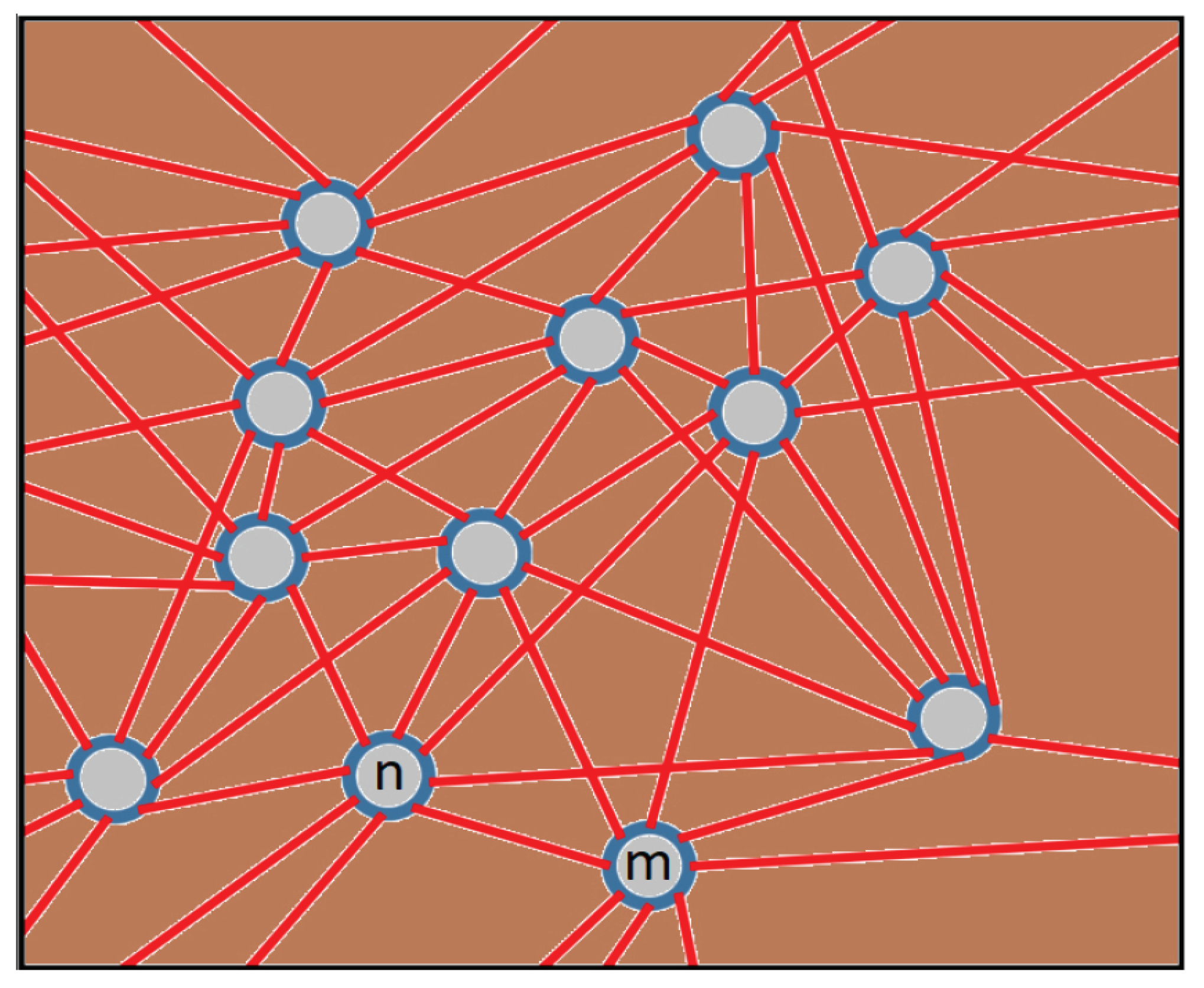
• the distance/length of the link;
• the angle of inclination of the link;
• the UGV itself; and
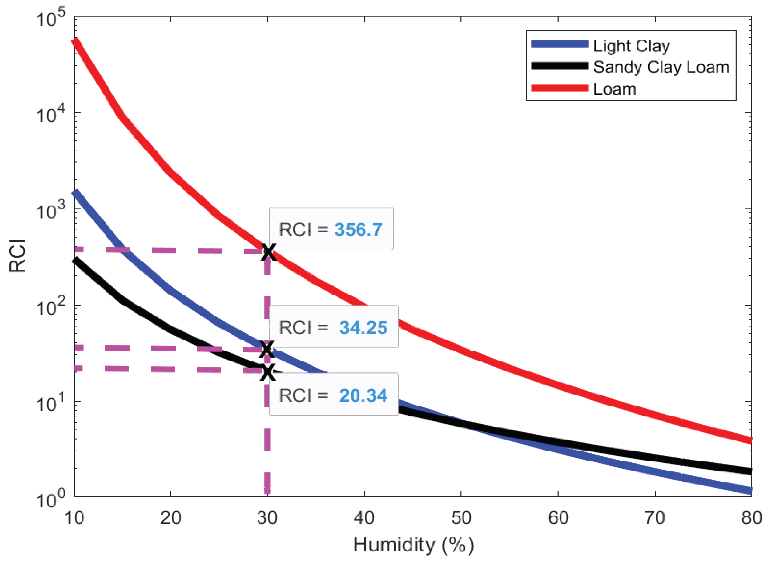
• the soil trafficability component (RCI), which depends on the weather humidity conditions.

The first three factors above are clearly fixed and are assumed to be known in advance. Factor (4) depends on the weather humidity conditions, and can be calculated using Figure 2 and following the techniques in [21,26]. This justifies the assumption that the energy costs (8) are available prior to navigation. If the weather humidity conditions change, it is possible to dynamically update the RCI values depending on the current weather humidity. Consequently, the energy-cost (8) and composite metric values (11) for the terrain links can be updated as well. As will be seen in the next section, Algorithm 1 terminates in a few seconds for soil graphs with thousands of nodes and tens of thousands of links. Thus, the algorithm can be re-invoked dynamically whenever the weather humidity conditions change.

4. Results and Discussion

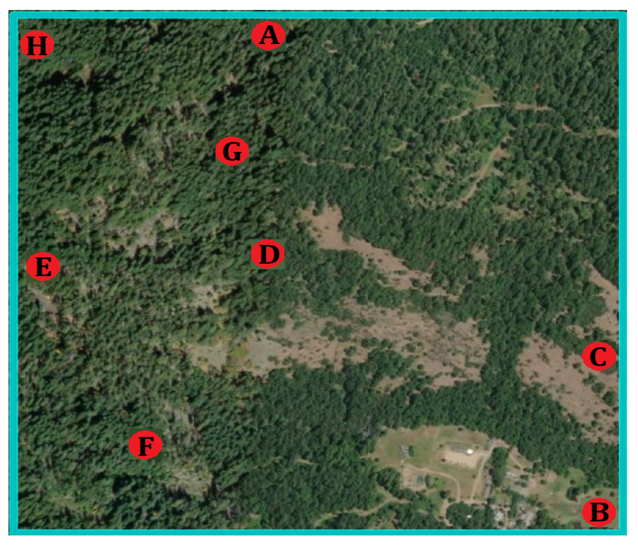
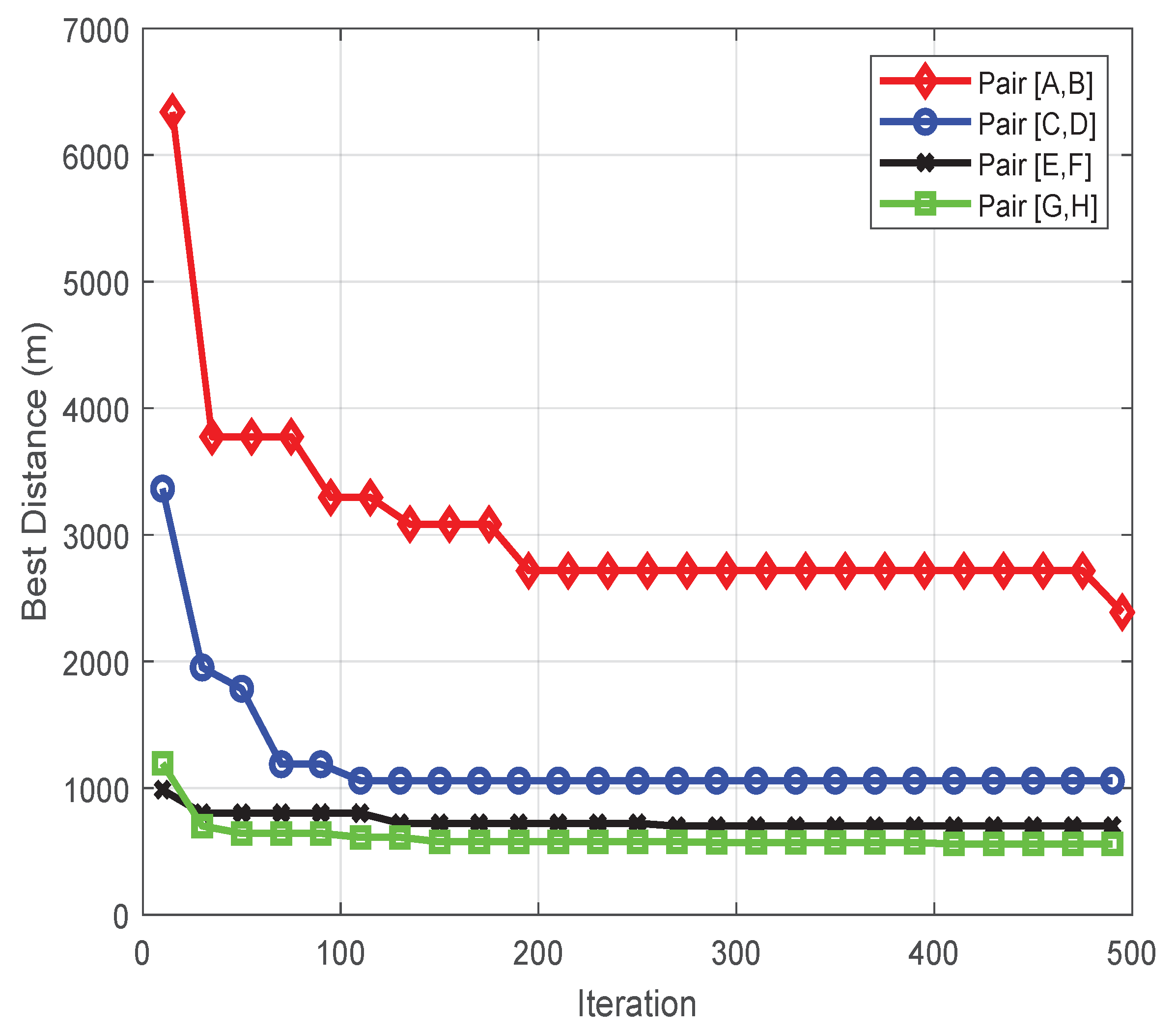
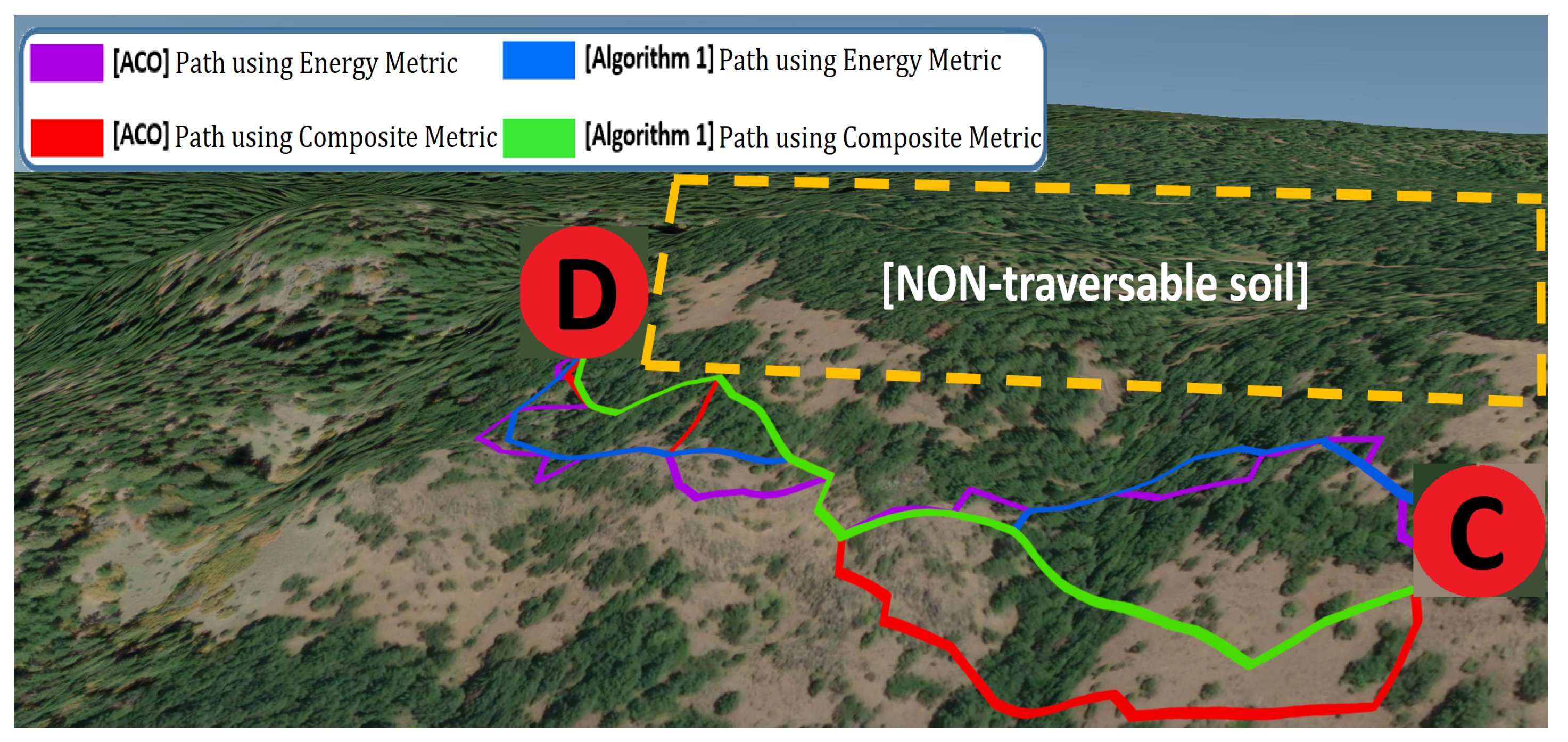
4.1. Benchmarks for Comparison

To quantify the performance of our proposed composite metric approach, we compare Algorithm 1 against the following benchmarks:

• The energy minimization routing approach from [22];
• The ACO meta-heuristic approach from [21].

It is worth noting that the study in [22] presented a routing algorithm that minimizes the energy consumption using an $A^{*}$-like algorithm. In fact, the $A^{*}$ algorithm attempts to reduce the number of Dijkstra iterations, at the expense of possible sub-optimal results when the $A^{*}$ is guided by an admissible heuristic [22]. As a benchmark for comparison, we minimize the energy consumption metric of [22] via a Dijkstra algorithm. Thereby, we are essentially comparing against the best possible results achievable by the approach of [22].

Note also that the ACO parameter values have been optimized in [21]. However, in this work we validate the optimal values of the parameters that produce the best possible results with fast convergence.

4.2. Test Setup

We first describe the environment of our work for carrying out simulations of the developed path planning algorithm. In this work, a square area of size 1.5 ${km}^2$ was chosen for our tests. The selected area is a section from Beiberstedt Butte summit, located in Oregon, USA. The reason behind our selection is that this summit is composed of a variety of soil types, some of which are nontraversable by the UGV type selected in this work. Secondly, this summit is rough and experiences elevation differences, which is a good example over UGV deployment and navigation in real-life under harsh conditions. The corresponding DEM map to the area under study, referred to in Figure 4, contains 2500 randomly-generated nodes, where each node has eight adjacent neighbors connected via links with a minimum of three meters spacing. We can also see a satellite image of the same area in Figure 5. Moreover, this section of the summit has a peak height of 1412 m, while the lowest point on it is 1039 m above sea level.

It was possible for us to generate this DEM map with its corresponding soil data by using the publicly available geological data from the U.S. Geographical Survey (USGS) agency. These data were utilized in ArcGis Pro and MATLAB R2018a programs for simulations. The simulations were carried on a desktop computer with the following specifications: six core 1.7 GHz Intel Xeon Bronze 3104 CPU with 16 GB RAM memory. In a similar fashion to [22], we set the UGV’s mass to 300 kg without any payload and its constant velocity to $0.5$ m/s. The static and dynamic friction coefficients are selected to be 1 and $0.1$, respectively. The UGV’s maximum power output is assumed to be $P_{max}$= 1280 W. To appropriately select the UGV’s VCI value that reflects real-life scenario deployment, we assume the UGV has the structure of an M1 tank (which has been tested and proven in [26] to be good at off-road navigation) with $VCI=26.34$ for single crossings over terrain. A single UGV crossing over a certain soil spot is a safe assumption to make because our simulation results show that there are barely any nodes being revisited throughout all the simulation runs. However, it should be said that the higher the number of UGV crossings on the same terrain, the higher the UGV VCI will be. Additionally, the chosen $VCI$ value, according to (1), justifies why $Type B$ soil area in Figure 4 is nontraversable, as in this scenario, $VCI > RCI$.

4.3. Simulation Results

We compare the greedy implementation of the proposed composite metric against the energy-cost minimization approach of [22], over multiple paths on the terrain under consideration to cover multiple UGV crossing scenarios. The greedy implementation of the proposed composite metric is deterministic in nature and produces solutions that do not change after running different simulations over the same input data. In fact, the obtained solution is optimal in the majority of the experiments. Simulation results for this part of the experiments are placed in

Table 1. Comparison against energy-cost minimization of [22].

Route Pair [s, f]	Path Length (m) and Energy (kJ) Resulting from [22]		Path Length (m) and Energy (kJ) Resulting from Algorithm 1		Path Length Reduction (Due to Algorithm 1)	Additional Energy Cost (Due to Algorithm 1)	Elapsed Time for [22]	Elapsed Time for Algorithm 1
	(m)	(kJ)	(m)	(kJ)	(%)	(%)	(s)	(s)
[A,B]	1989.2	97.7	1828.9	98.5	8.06	0.80	3.35	3.42
[C,D]	1024.2	579.4	911	601.3	11.05	3.65	3.16	3.22
[E,F]	806.6	51	663.6	52.8	17.73	3.45	3.24	3.43
[G,H]	526.3	274	490.9	279.2	6.73	1.86	3.30	3.49

. We consider running and comparing the proposed algorithm over four different UGV way points. Each path is represented by denoting its starting and finishing nodes as pairs of letters [$start$, $finish$]. It should be said that the selected pairs are randomly chosen and vary significantly in path distance to test our proposed algorithm under different scenarios.

The metrics used to assess the quality of each obtained path are the path length representing the terrain distance crossed by the UGV in meters (m) and the energy consumed by UGV batteries to traverse that path in kilo Joules (kJ). We also calculated the percentage difference between the length and energy consumption of the paths obtained using the energy-cost metric of [22] relative to those obtained using the proposed composite metric. Finally, we also assessed the algorithm running time for both approaches. Table 1 clearly indicates the superiority of our proposed composite metric-based algorithm over the pure energy minimization algorithm in terms of the total path length reduction. Moreover, the cost of this distance reduction is barely noticeable as a small increase in the energy consumption of the proposed algorithm. This is best demonstrated in the [E, F] route pair, where a noticeable $17.7\%$ distance reduction was achieved via the proposed algorithm with a marginal added energy consumption of less than $3.5\%$. In some cases, the increase in energy was next to zero as in the [A, B] route pair, where there is a pure $8\%$ distance reduction, with less than $1\%$ additional energy cost. We can also notice that the gain in distance reduction is not linearly proportionate with the increase in energy consumption. For example, in both [C, D] and [E, F] route pairs, the additional energy costs are almost the same, while the reduction in path length varied from $11\%$ to $17.7\%$, respectively. Finally, we show that the running time of both algorithms is almost matching and relatively small, with an average higher run time of $3.9\%$ for the proposed algorithm. We can deduce from this the fact that the introduced composite metric barely adds to the overall computational complexity.

Table 2. Ant Colony Optimization (ACO) results and comparison.

Route Pair [s, f]	Path Length (m) and Energy (kJ) Resulting from ACO		Path Length Reduction (Due to Algorithm 1)	Energy-Cost Reduction (Due to Algorithm 1)	Elapsed Time for ACO
	(m)	(kJ)	(%)	(%)	After 100 ite. (s)	After 500 ite. (s)
[A,B]	2388.3	296.8	23.38	66.81	58 230	230
[C,D]	1058.7	666.7	13.95	9.81	33	105
[E,F]	699.6	68.9	5.15	23.37	30	90
[G,H]	558.1	287.5	12.04	2.89	23	55

summarizes the results obtained using the ACO approach of [21] and how these results compare against the proposed greedy algorithm (i.e., Algorithm 1). It is clearly seen that our proposed greedy composite metric approach provides superior results, in terms of the distance and energy consumption of the obtained paths, and also in terms of the algorithm running time. In particular, the proposed greedy approach resulted in paths with up to $23\%$ shorter distances, and up to staggering $67\%$ lower energy consumption, with a reduction one to two orders of magnitude in the algorithm running time. It is worth noting that the benchmark ACO implementation also uses the same composite metric as a routing objective. This justifies why the greedy algorithm performs better on both fronts, i.e., the path distance and energy consumption. The results in Table 1, however, compare the composite metric against pure energy minimization. The latter leads to the tradeoff of reducing the resulting path distance at the expense of a slight increase in the energy consumption.

Finally, Figure 6 and Figure 7 depict the convergence of the ACO algorithms in terms of the path distance and energy consumption, respectively. Moreover, Figure 8 shows the final constructed paths from the greedy and ACO implementations for the [C, D] routing pair projected on a 3D terrain that corresponds to the real-life mountainous area under consideration in this work. By analyzing Figure 6 and Figure 7, we can clearly see that the number of ACO iterations required for path planning convergence to a final or near-final path length and energy cost values is roughly between 100–200 iterations, depending on the UGV route under planning. To achieve the best possible ACO results for comparison purposes, we consider 500 iterations for all ACO runs, which under some paths can produce slightly better results over the first 100–200 iterations. It should be also noted that we performed tests up to 1000 iterations, and we did not record any improvements as compared to the 500th iteration and onwards. It is intelligible from Figure 8 that all the constructed paths are avoiding the nontraversable soil (upper side to the constructed routes) and only consider reaching the final destination (D) node by moving forward and descending.

5. Conclusions

This paper proposes a composite metric routing approach based on combining the distance and energy of the routing path for solving the problem of energy-efficient path planning for UGVs (unmanned ground vehicles) on natural off-road uneven mountainous real-life terrain. We present a greedy implementation of the composite metric approach. Additionally, the Terramechanics of the surface of the terrain between the UGV wheels and the soil is taken into account. The terrain slope is considered in the energy model to account for the UGV capability of passing over, based on the available power stored in the UGV batteries. As benchmarks for comparison, we use a recent energy minimization approach, in addition to an ant colony optimization (ACO) meta-heuristic. The observed results show that, under the composite metric greedy implementation, a better performance can be achieved in terms of creating shorter paths compared to directly minimizing the energy cost, with a negligible increase in the energy consumption. In fact, in some route pairs, the composite metric achieves a respectable $17.7\%$ distance reduction with only a small energy consumption penalty of $3.5\%$ compared to direct energy minimization. Moreover, our results also indicate that the proposed greedy algorithm strongly outperforms the ACO implementation in terms of the quality of the paths obtained and the algorithm running time. In fact, the running time of our proposed algorithm indicates its suitability for large natural terrain graphs with thousands of nodes and tens of thousands of links. Avenues for future research include relaxing the condition that the UGV velocity is constant and incorporating the energy consumption due to acceleration and deceleration in the model and algorithm.

References

1. Leighty, R.D. Terrain navigation concepts for autonomous vehicles. In Applications of Artificial Intelligence I; International Society for Optics and Photonics: Bellingham, WA, USA, 1984; Volume 485, pp. 120–125. [Google Scholar]
2. Yaqoob, I.; Khan, L.U.; Kazmi, S.A.; Imran, M.; Guizani, N.; Hong, C.S. Autonomous driving cars in smart cities: Recent advances, requirements, and challenges. IEEE Netw. 2019, 34, 174–181. [Google Scholar] [CrossRef]
3. Huang, H.; Savkin, A.V.; Ding, M.; Huang, C. Mobile robots in wireless sensor networks: A survey on tasks. Comput. Netw. 2019, 148, 1–19. [Google Scholar] [CrossRef]
4. Bold, S.; Sosorbaram, B.; Lee, S.R. Implementation of autonomous unmanned aerial vehicle with moving-object detection and face recognition. In Information Science and Applications (ICISA) 2016; Springer: Berlin, Germany, 2016; pp. 361–370. [Google Scholar]
5. Yan, C.; Xiang, X.; Wang, C. Towards real-time path planning through deep reinforcement learning for a uav in dynamic environments. J. Intell. Robot. Syst. 2020, 98, 297–309. [Google Scholar] [CrossRef]
6. Ganganath, N.; Cheng, C.T.; Fernando, T.; Iu, H.H.; Tse, C.K. Shortest Path Planning for Energy-Constrained Mobile Platforms Navigating on Uneven Terrains. IEEE Trans. Ind. Inform. 2018, 14, 4264–4272. [Google Scholar] [CrossRef]
7. Wu, C.; Dai, C.; Gong, X.; Liu, Y.J.; Wang, J.; Gu, X.; Wang, C.C. Energy-Efficient Coverage Path Planning for General Terrain Surfaces. IEEE Robot. Autom. Lett. 2019, 4, 2584–2591. [Google Scholar] [CrossRef]
8. Comin, F.J.; Lewinger, W.A.; Saaj, C.M.; Matthews, M.C. Trafficability assessment of deformable terrain through hybrid wheel-leg sinkage detection. J. Field Robot. 2017, 34, 451–476. [Google Scholar] [CrossRef] [Green Version]
9. Priddy, J.D.; Willoughby, W.E. Clarification of vehicle cone index with reference to mean maximum pressure. J. Terramech. 2006, 43, 85–96. [Google Scholar] [CrossRef]
10. Kim, S.; Jin, H.; Seo, M.; Har, D. Optimal Path Planning of Automated Guided Vehicle using Dijkstra Algorithm under Dynamic Conditions. In Proceedings of the 2019 7th International Conference on Robot Intelligence Technology and Applications (RiTA), Daejeon, Korea, 1–3 November 2019; pp. 231–236. [Google Scholar]
11. Wei, M.; Isler, V. Energy-efficient Path Planning for Ground Robots by and Combining Air and Ground Measurements. In Proceedings of the Conference on Robot Learning, Cambridge, MA, USA, 14–16 November 2020; pp. 766–775. [Google Scholar]
12. Aksamentov, E.; Zakharov, K.; Tolopilo, D.; Usina, E. Approach to robotic mobile platform path planning upon analysis of aerial imaging data. In Proceedings of the 15th International Conference on Electromechanics and Robotics “Zavalishin’s Readings”; Springer: Berlin, Germany, 2020; pp. 93–103. [Google Scholar]
13. Wallace, N.D.; Kong, H.; Hill, A.J.; Sukkarieh, S. Energy Aware Mission Planning for WMRs on Uneven Terrains. IFAC-PapersOnLine 2019, 52, 149–154. [Google Scholar] [CrossRef]
14. Taghavifar, H.; Xu, B.; Taghavifar, L.; Qin, Y. Optimal Path-Planning of Nonholonomic Terrain Robots for Dynamic Obstacle Avoidance Using Single-Time Velocity Estimator and Reinforcement Learning Approach. IEEE Access 2019, 7, 159347–159356. [Google Scholar] [CrossRef]
15. Xin, J.; Wei, L.; Wang, D.; Xuan, H. Receding horizon path planning of automated guided vehicles using a time-space network model. Optim. Control. Appl. Methods 2020, 41, 1889–1903. [Google Scholar] [CrossRef]
16. Herrmann, T.; Wischnewski, A.; Hermansdorfer, L.; Betz, J.; Lienkamp, M. Real-Time Adaptive Velocity Optimization for Autonomous Electric Cars at the Limits of Handling. IEEE Trans. Intell. Veh. 2020. [Google Scholar] [CrossRef]
17. Herrmann, T.; Passigato, F.; Betz, J.; Lienkamp, M. Minimum Race-Time Planning-Strategy for an Autonomous Electric Racecar. In Proceedings of the 2020 IEEE 23rd International Conference on Intelligent Transportation Systems (ITSC), Rhodes, Greece, 20–23 September 2020; pp. 1–6. [Google Scholar]
18. Ebbesen, S.; Salazar, M.; Elbert, P.; Bussi, C.; Onder, C.H. Time-optimal control strategies for a hybrid electric race car. IEEE Trans. Control. Syst. Technol. 2017, 26, 233–247. [Google Scholar] [CrossRef]
19. Hu, X.; Chen, L.; Tang, B.; Cao, D.; He, H. Dynamic path planning for autonomous driving on various roads with avoidance of static and moving obstacles. Mech. Syst. Signal Process. 2018, 100, 482–500. [Google Scholar] [CrossRef]
20. Zhang, Y.; Chen, H.; Waslander, S.L.; Gong, J.; Xiong, G.; Yang, T.; Liu, K. Hybrid trajectory planning for autonomous driving in highly constrained environments. IEEE Access 2018, 6, 32800–32819. [Google Scholar] [CrossRef]
21. Wang, H.; Zhang, H.; Wang, K.; Zhang, C.; Yin, C.; Kang, X. Off-road path planning based on improved ant colony algorithm. Wirel. Pers. Commun. 2018, 102, 1705–1721. [Google Scholar] [CrossRef]
22. Ganganath, N.; Cheng, C.T.; Tse, C.K. A constraint-aware heuristic path planner for finding energy-efficient paths on uneven terrains. IEEE Trans. Ind. Inform. 2015, 11, 601–611. [Google Scholar] [CrossRef] [Green Version]
23. Saad, M.; Salameh, A.I.; Abdallah, S. Energy-efficient shortest path planning on uneven terrains: A composite routing metric approach. In Proceedings of the 2019 IEEE International Symposium on Signal Processing and Information Technology (ISSPIT), Ajman, United Arab Emirates, 10–12 December 2019; pp. 1–6. [Google Scholar]
24. Dorigo, M.; Birattari, M.; Stutzle, T. Ant colony optimization. IEEE Comput. Intell. Mag. 2006, 1, 28–39. [Google Scholar] [CrossRef] [Green Version]
25. Winterkorn, H.F.; Fang, H.Y. Soil technology and engineering properties of soils. In Foundation Engineering Handbook; Springer: Berlin, Germany, 1991; pp. 88–143. [Google Scholar]
26. Ciobotaru, T. Semi-empiric algorithm for assessment of the vehicle mobility. Leonardo Electron. J. Pract. Technol. 2009, 8, 19–30. [Google Scholar]
27. Rowe, N.C.; Ross, R.S. Optimal grid-free path planning across arbitrarily contoured terrain with anisotropic friction and gravity effects. IEEE Trans. Robot. Autom. 1990, 6, 540–553. [Google Scholar] [CrossRef]
28. Rula, A.A.; Nuttall, C.J., Jr. An Analysis of Ground Mobility Models (ANAMOB); Technical Report; Army Engineer Waterways Experiment Station Vicksburg Ms: Vicksburg, MS, USA, 1971. [Google Scholar]
29. Sun, Z.; Reif, J.H. On finding energy-minimizing paths on terrains. IEEE Trans. Robot. 2005, 21, 102–114. [Google Scholar]
30. Sobrinho, J.L. An algebraic theory of dynamic network routing. IEEE/ACM Trans. Netw. 2005, 13, 1160–1173. [Google Scholar] [CrossRef]
31. Saad, M. Non-isotonic routing metrics solvable to optimality via shortest path. Comput. Netw. 2018, 145, 89–95. [Google Scholar] [CrossRef]
Figure 1. The three types of soil found in the real-life terrain employed for UGV routing in this paper.
Applsci 11 06939 g001
Figure 2. RCI values plotted against different humidity conditions for the three soil types found in the real-life terrain considered in this paper.
Applsci 11 06939 g002
Figure 3. A visual representation of the graph that represents the simulated terrain.
Applsci 11 06939 g003
Figure 4. The area under study represented as a DEM map with information about soil type. The red dots represent the nodes visited by the UGV along its movement to the destination.
Applsci 11 06939 g004
Figure 5. 2D satellite imagery of the area under study with 4 UGV paths defined by their starting and ending positions as letters (pairs of two letters).
Applsci 11 06939 g005
Figure 6. Convergence of the path distance vs. the ACO iterations.
Applsci 11 06939 g006
Figure 7. Convergence of the path energy vs. the ACO iterations.
Applsci 11 06939 g007
Figure 8. A 3D terrain model that displays the constructed paths from using the greedy (Algorithm 1) and ACO implementation simulation results for the [C, D] route pair over the real-life land under consideration in this work.
Applsci 11 06939 g008