Article

Noisy Optimization of Dispatching Policy for the Cranes at the Storage Yard in an Automated Container Terminal

1
Department of Information Convergence Engineering, Pusan National University, Busan 46241, Korea
2
Department of Computer & Telecommunications Engineering, Yonsei University, Wonju 26493, Korea
3
Hyundai Motors Company, Seoul 06797, Korea
4
School of Computer Science and Engineering, Pusan National University, Busan 46241, Korea
*
Author to whom correspondence should be addressed.
Appl. Sci. 2021, 11(15), 6922; https://doi.org/10.3390/app11156922
Submission received: 5 June 2021 / Revised: 16 July 2021 / Accepted: 28 July 2021 / Published: 28 July 2021

Abstract

:
In this paper, we claim that the operation schedule of automated stacking cranes (ASC) in the storage yard of automated container terminals can be built effectively and efficiently by using a crane dispatching policy, and propose a noisy optimization algorithm named N-RTS that can derive such a policy efficiently. To select a job for an ASC, our dispatching policy uses a multi-criteria scoring function to calculate the score of each candidate job using a weighted summation of the evaluations in those criteria. As the calculated score depends on the respective weights of these criteria, and thus a different weight vector gives rise to a different best candidate, a weight vector can be deemed as a policy. A good weight vector, or policy, can be found by a simulation-based search where a candidate policy is evaluated through a computationally expensive simulation of applying the policy to some operation scenarios. We may simplify the simulation to save time but at the cost of sacrificing the evaluation accuracy. N-RTS copes with this dilemma by maintaining a good balance between exploration and exploitation. Experimental results show that the policy derived by N-RTS outperforms other ASC scheduling methods. We also conducted additional experiments using some benchmark functions to validate the performance of N-RTS.

1. Introduction

The storage yard of an automated container terminal is a buffer area where the import and export containers are stored temporarily. The import containers, after being discharged from the vessels, are delivered to the storage yard and then stored there until they are carried out for road or rail transportation. The export containers carried in from the inland dwell at the storage yard until they are loaded onto vessels for sea transportation. Being an interface between the seaside and the landside, the storage yard often becomes a bottleneck for the whole logistics flow within a terminal. The delay of vessel operations caused by the delayed operations at the storage yard is among the major obstacles of enhancing the productivity of a terminal. The storage yard of an automated container terminal usually consists of dozens of rectangular blocks, each of which accommodates hundreds of container stacks. Each block is typically equipped with two rail-mounted, automated stacking cranes (ASC) for container handling. These two ASCs are usually of an equal size and cannot move across each other, thus being prone to mutual interference at close range. For efficient operations at a block, these ASCs need to be carefully scheduled to process the requested jobs, so that the cooperation between the two ASCs is maximized, while minimizing the interferences. In this paper, we tried to achieve this goal by optimizing the crane dispatching policy that decides which ASC should process which job, in which order.
The crane dispatching policy recommends a job to be conducted next by the ASC that has just finished its previously assigned job. If the policy can recommend the jobs to the ASCs in such a way that the workloads of the two ASCs are as balanced as possible (and the interferences are minimized), then the crane utilization can be maximized [1]. Many previous works on crane scheduling take the approach of rolling horizon search, in which an optimal crane schedule (to process the jobs within a horizon) is searched repeatedly, at regular intervals [1,2,3,4,5,6,7]. Although better than those obtained with simple heuristic dispatching rules, the crane schedules obtained with the rolling horizon approach can still be myopic, due to the rather short length of the scheduling horizon. Increasing the length of the horizon, however, is not easy as the search space becomes large, and thus, the problem cannot be solved (i.e., cranes cannot be scheduled) in real time under an online setting. Our crane dispatching policy has the potential to overcome the problem of making myopic decisions, as it is optimized through an offline search, in which each candidate policy is evaluated through simulations of diverse (and long enough) scenarios of operations at a block.
The crane dispatching policy proposed in this paper can be viewed as a multi-criteria heuristic. Unlike simple heuristics, such as the earliest-deadline-first or nearest-job-first heuristics, that are based on a single criterion, our policy uses a multi-criteria scoring function to make a selection from various candidate choices. This scoring function calculates the score of each candidate choice by a weighted summation of the evaluations on multiple criteria, each of which was designed to measure how good a choice was, from its own perspective. The score by weighted summation depends on the respective weights of these criteria, and thus, a different weight vector gives rise to a different best candidate, a weight vector can be deemed as a dispatching policy. To find a good policy, we conducted a search in the space of weight vectors, i.e., in the policy space, where a candidate weight vector was evaluated by applying the corresponding scoring function to decision makings for dispatching in various operational scenarios and observing the resulting performance. If these training scenarios are long and diverse enough, we can learn a good policy that is not myopic, but at the cost of a long computation time. Although this offline policy search can be somewhat computationally expensive, the obtained policy is very quick and powerful in usage. When used for crane dispatching, the scoring function based policy would involve only slightly more computation than the simple heuristics but would be orders of magnitude faster than the online rolling horizon search methods. Nevertheless, its decision-making quality was better than that of the online search method, as seen later in our report of experimental results.
One difficulty with the search for an optimal policy was that the evaluation of even one candidate policy (i.e., a weight vector) takes a long time, due to the long simulations involved. If we make the simulation quicker, by reducing the simulation scenarios in an attempt to save the computation time, the resulting evaluation becomes inaccurate or noisy. There has been some previous work on noisy optimization techniques [8,9,10,11,12,13,14] that deal with this type of problem. Their basic approach is not to try to evaluate every candidate very accurately, but to evaluate some candidates approximately to save computational resources, unless their quality appears reasonable. In this paper, we propose a noisy optimization algorithm named N-RTS that is a major improvement of the NTGA algorithm [12,15], and we used this algorithm to optimize our crane dispatching policy. The performance of N-RTS was verified by comparative experiments with other competing methods. We also conducted additional experiments using several benchmark noisy optimization problems and confirmed the performance improvement achieved by N-RTS. Some test results with a preliminary version of N-RTS, using the same set of benchmark problems, can be found in [16].
The rest of the paper is organized as follows. The next section provides a detailed description of the crane operations at a storage block of an automated container terminal. Section 3 reviews the related works. Section 4 explains how the crane dispatching policy works for the crane operations and then describes the noisy optimization algorithm that can optimize the policy. Section 5 reports the results of the experiments. Section 6 provides the summary and conclusions.

2. Operations of Automated Stacking Cranes

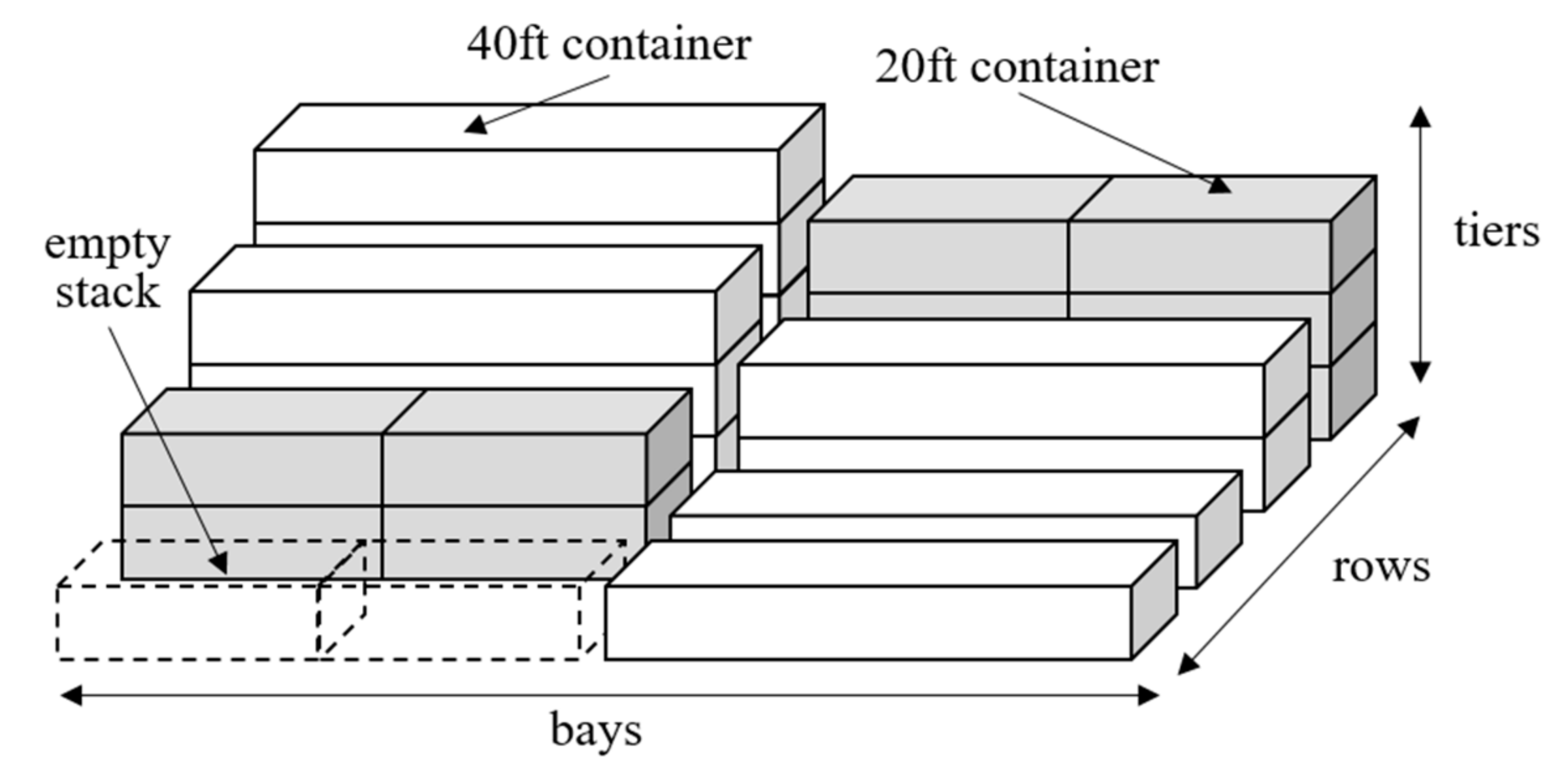
The content in this section is largely based on the materials provided in the work of Choe et al. (2015). Figure 1 presents the layout of a typical automated container terminal, showing the quayside, the apron area, the hinterland area, and some blocks in the storage yard, where each block is illustrated shorter than its reality (in the longitudinal direction). Figure 2 shows the structure of a block in detail. It should be noted that the horizontal direction in Figure 2 corresponds to the longitudinal direction in Figure 1. A block is laid out perpendicularly to the quay and accommodates hundreds of container stacks that are several tiers high, which are arranged in dozens of bays in the perpendicular direction and in several rows in the horizontal direction. Since one bay is the length of a 20 ft container, a stack of 40 ft containers spans two consecutive bays. The containers of different sizes cannot be stacked together for safety reasons. The containers stored at a block can be categorized into three groups, according to their directions of logistics flow: import, export, and transshipment containers. The import and export containers were already explained at the beginning of the previous section. The transshipment containers, similar to the import containers, are discharged from the vessels by the quay cranes (QC) and stored at the yard; later, they are loaded onto other vessels for further sea transportation. In the apron area, the automated guided vehicles (AGV) deliver the containers between the QCs and ASCs. The container handover between an AGV and an ASC takes place at a handover point (HP), provided at the seaside end of a block. The containers transported to/from inland are carried by external trucks (ET). The container handover between an ET and an ASC takes place at an HP at the landside end of a block.
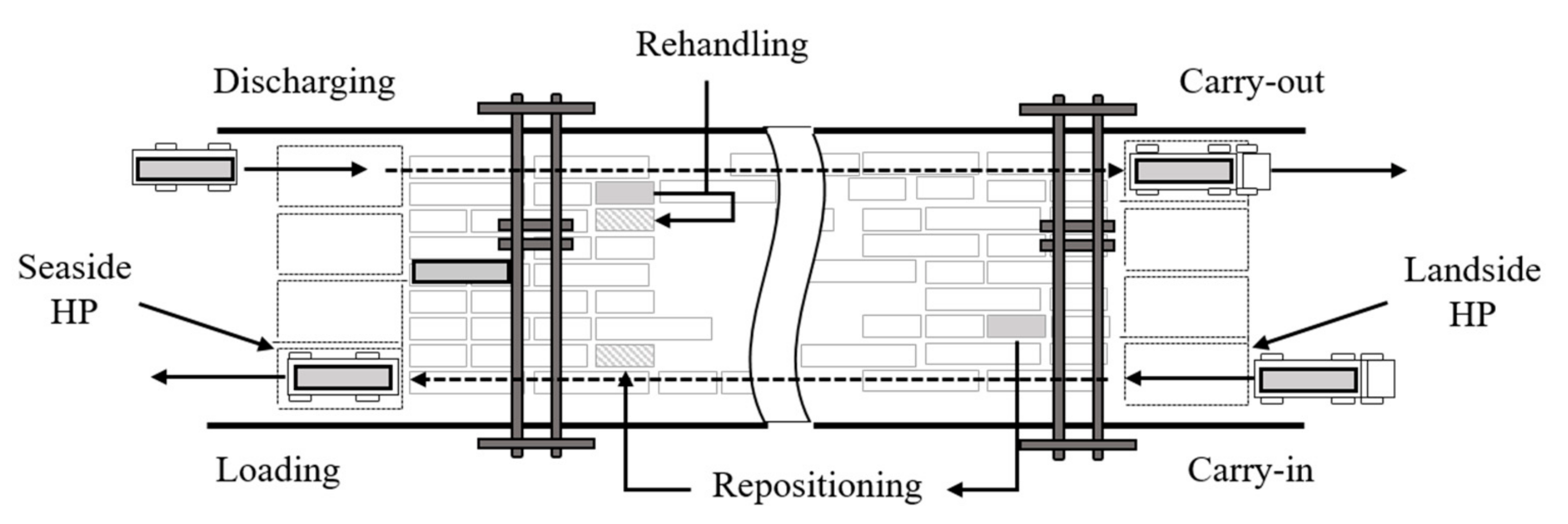
The main jobs performed by the ASCs can be categorized into four types: loading, discharging, carry-in, and carry-out, as indicated in Figure 3. The loading and discharging jobs are also called the seaside jobs, and the carry-in and carry-out jobs are called the landside jobs. The seaside jobs, unlike the landside jobs, have deadlines imposed by the discharging and loading plans for the vessels at the berths. In any container terminal, the sequences for discharging and loading the containers from and to a vessel are predetermined during the planning phase, before the operation for the vessel starts. Typically, each vessel is serviced by multiple QCs, for each of which the discharging and/or loading sequences are determined. When a QC starts its discharging or loading operation, each container in the sequence can be assigned a deadline or a due time by considering the QC cycle time for the respective container. By this deadline, an AGV must be made ready under the QC to receive or release a container, in order not to have the QC delayed. Once the deadlines under the QC are determined, the estimated deadlines for the corresponding seaside jobs at the blocks can be set up by taking account of the average travel speed of the AGVs and the distances from the QC to the blocks. QC deadlines should be updated whenever a delay occurs, as the QC cycle times cannot be shortened, and thus, the containers thereafter cannot help being delayed, either. In addition to the main jobs, the ASCs also perform the preparatory jobs, such as the rehandling or repositioning jobs, to be explained soon. Since the two ASCs in a block cannot move across each other, the seaside jobs are exclusively serviced by the seaside ASC (and the landside jobs by the landside ASC). An ASC goes through four consecutive steps of movement to accomplish any container handling job: empty travel to the target container, picking up the container, loaded travel to the destination, and dropping off the container. For a discharging job, the seaside ASC picks up an import or transshipment container from an AGV at a seaside HP and stacks it at a designated position in the block. For a loading job, the seaside ASC picks up an export or transshipment container from a stack in the block and loads it onto an AGV waiting at a seaside HP. For carry-in or carry-out jobs, the landside ASC works in similar ways to receive an export container from, or release an import container to, an ET at a landside HP, respectively.
It is noteworthy that a container entering a block through one end of a block later exits through the opposite end of the block, unless it is a transshipment container. This implies that the container cannot help being handled by both the landside and seaside ASCs. Suppose an export container, carried in by an ET, has arrived at a landside HP of a block. Then, the landside ASC picks it up and may put it down on a stack close to the landside end of a block to save time. When this container has to be loaded onto a vessel, it may not be desirable for the seaside ASC to directly come to pick up the container, due to the risk of interference with the landside ASC. A better option would be to move the container toward the seaside through cooperation between the two ASCs. First, for example, the landside ASC moves the container to a stack located approximately halfway to the seaside HP. An attempt to move it too close to the seaside can lead to an ASC interference. Later, the seaside ASC picks up the container and loads it onto an AGV waiting at a seaside HP. The first preparatory movement, made by the landside ASC in this example scenario, is called repositioning (see Figure 3). When some containers are stacked on top of a target container to be picked up, those above should be moved away before the targeted one can be retrieved. This so-called rehandling is also one of the major causes of operational delay at the block. While repositioning tends to move the target container as far away as possible, the rehandled containers are usually moved to nearby locations so that the target container below can be picked up as quickly as possible. Although the seaside jobs and landside jobs can only be performed exclusively by the seaside ASC and landside ASC, respectively, rehandling and repositioning jobs can be done by either of the two ASCs. In fact, the workloads of the two ASCs can be better balanced by having a less heavily loaded ASC perform more of the preparatory jobs, i.e., the rehandling and repositioning jobs [1].
The efficiency of the loading operation is considered the most critical to the productivity of the whole terminal, as the turnaround time of a vessel depends on how fast the containers are loaded. However, fast loading is not always easy, due to the frequent rehandling and repositioning situations that arise during loading. To minimize the delays incurred by rehandling or repositioning during loading, the relevant containers are often rearranged before loading operation starts. If such a preparatory task, called remarshaling, can be performed in advance for a large portion of the containers to be loaded onto an upcoming vessel, the loading operation for that vessel will be highly expedited. To have as many remarshaling jobs performed as possible, the ASCs should be operated in such a way that any idle times between the jobs of the containers for the current vessels are maximally utilized for the remarshaling of the containers for the upcoming vessels. The containers to be rearranged for remarshaling also include the import containers currently stored in the seaside area of the block that are estimated to be carried out by ETs during the same period of loading operation for an upcoming vessel. The relocation of these import containers to positions closer to the landside end of the block will not only facilitate the corresponding future carry-out operations, but also provide more space at the seaside area to accommodate the containers to be remarshaled to the seaside for future loading.
The performance of ASCs at a block is measured by the average AGV delay and ET waiting time. Since each seaside job has a deadline, a delayed operation of the seaside ASC results in an AGV delay and, eventually, a QC delay. A retarded operation of the landside ASC causes an ET to wait longer. We do not call this tardiness a delay, as the landside jobs do not have any explicit deadline. While the most important operational goal is to minimize the AGV delay at the seaside HPs (and thus, to minimize the vessel turnaround times), the waiting time of ETs at the landside HPs should not be sacrificed too much to provide reasonable services to ETs. The objective function for the optimization of ASC operation is thus given as a weighted sum of the average AGV delay and average ET waiting time per container, where the weight for the AGV delay is usually much larger than that for ET waiting time.

3. Related Work

Most previous work on scheduling the stacking cranes has investigated plan (or schedule) search methods for determining the order of processing the container jobs requested within a fixed-length horizon. Since the search space becomes very large as the horizon becomes longer, some studies focus on finding a good plan within a rather short horizon [2,3,6], and some others try to cope with the search space by employing various techniques, such as branch-and-bound and its variants [2,7] or local-search-based methods [1,3,4,6]. Although a plan derived from a short horizon can be myopic, a plan from too long a horizon is not necessarily desirable. The plan obtained from a long horizon may not be well-optimized, due to the large search space. Even if the plan is well-optimized, it can become obsolete before long under an uncertain environment. Since the arrival times of ETs and AGVs (or yard tractors in conventional terminals) cannot be predicted accurately and the crane operations cannot be exactly deterministic, an execution of a plan can quickly deviate from the expected outcome. This leads to the studies on the online rolling horizon search method that replans for a horizon at regular intervals, in which the replanning interval is usually much shorter than the length of the planning horizon [1,3,4,5,6,18].
Important issues of scheduling the twin ASCs include how the workloads of the two ASCs can be balanced through cooperation and how the interferences between them can be minimized. Park et al. [1] achieve good load balancing by treating the preparatory jobs (i.e., rehandling and repositioning jobs) as independent jobs, so that the ASC with a lower workload can process more of them. Gharehgozli et al. [19] reduced ASC interferences by defining the movement scheduling of the ASCs as a TSP problem, so that the minimum distance between the ASCs can be maintained. Briskorn et al. [18] proposed a scheduling method that enabled ASC jobs to be performed in a pipelining manner, in order to improve the repositioning efficiency. However, all these (and previously mentioned works) ignore the issue of remarshaling. Early studies on remarshaling unrealistically assume that a long enough period of crane idle time is available, during which all the remarshaling jobs can be completed in a batch [20,21]. A later work [22] deals with the problem of generating a selective remarshaling plan, under the constraint that the ASCs are idle for only a limited period of time. Nevertheless, this work assumes that the remarshaling works for a selected subset of containers that are performed in a batch. A more recent work [5] proposes a realistic ASC scheduling method, in which remarshaling jobs can be performed whenever the workloads of ASCs for the main jobs are light. Our work in this paper was an extension of the work in [5]. Instead of their plan to search under an online setting, however, we conducted an offline search for an optimal crane dispatching policy to be used for scheduling the ASCs online.
Most works on noisy optimization use evolutionary algorithms, where the key issue is how to allocate samples efficiently in evaluating candidate solutions. A baseline approach to noisy optimization would be to take a number of fitness samples and average them to achieve the maximum noise-cancelling effect. However, such simple repeated resampling does not allow an efficient exploration of the search space as the computation for evaluating each individual candidate is too heavy. The adaptive resampling methods [8,9,23,24] more effectively use the limited computational resources by dynamically adapting the number of samples during evolution. The duration-scheduling (DS) method [8] gradually increases the sample size at every generation but makes adjustments based on the estimated noise level of the current population, assuming a non-overlapping generation model. Pietro et al. [23] provided more samples to the candidates whose evaluation values showed larger standard deviations. The memetic differential evolution (MDE) algorithm [24] provides a single sample to newly born individuals for their initial evaluation. During the survival selection, both the competitors receive ns additional samples if their fitness difference is less than 2σ, where σ is the noise level assumed to be known and ns is determined as inversely proportional to the fitness difference. The winner keeps the samples, so that they can be reused together with the additional samples given in future rounds of survival selection. Later, this idea of sample accumulation was applied to the population of overlapping generation models or to archive noisy multi-objective evolutionary algorithms, in order to increase the reliability of the survival selection, as the competitors from the population have more samples accumulated to them [11,12,13,14,25].
Noisy RTS (N-RTS), that we propose in this paper, is built on top of the restricted tournament selection (RTS) algorithm [26], which is an overlapping population model adopting the crowding factor idea to maintain the population diversity. N-RTS also gives a minimum constant number of samples to newly born individuals for initial evaluation, but later strategically allots additional samples to the competitors, based on several probabilistic decisions. Of course, the allotted samples are accumulated to make subsequent evaluations more reliable.

4. Policy Optimization

Whenever an ASC finishes its current job, it refers to the crane dispatching policy to select its next job. In preparation for this selection, a set of candidate jobs that should (or can) be done within a fixed-length horizon are identified, as explained in detail in Section 4.1. If the candidate job is one of the retrieval jobs, the job is already well-defined as its pickup location (where the container is currently stacked), and its drop-off location is one of the HPs where the requesting vehicle is waiting. If not, the job must be defined by determining the stacking position for the corresponding container. In this paper, we used the stacking policy developed by [5] to determine the stacking position of a container, whether it is the one newly coming into the block or the one relocated within the block for rehandling, repositioning, or remarshaling. Similar to our crane dispatching policy, the stacking policy also uses a multi-criteria scoring function to evaluate candidate stacking positions and selects the best one. It is after the stacking positions are all determined that the crane dispatching policy evaluates each candidate job and assigns the best job to the waiting ASC. After each dispatching of ASC, the horizon and the corresponding set of candidate jobs are updated, and the stacking policy followed by the dispatching policy is referenced again. Figure 4 provides the pseudocode for the overall procedure of ASC operations at a block. Below, we first describe how we uses a multi-criteria scoring function to create the crane dispatching policy. In the subsections that follow, we explain how the policy can be optimized by using our noisy optimization technique.

4.1. Crane Dispatching Policy

Now, we describe the crane dispatching policy that uses a scoring function to evaluate each candidate job and recommends the one with the best score to the ASC. The set J of candidate jobs is obtained by taking a union of the set M of the main jobs, the set P of the preparatory jobs, and the set R of the remarshaling jobs, as suggested in [5]:
J = MPR
M consists of the discharging, loading, carry-in, and carry-out jobs that are requested within the current horizon. The discharging and loading requests are generated from the discharging and loading plans for the vessels at the berths. The discharging and loading jobs in M cannot be for just a single QC, but for multiple QCs. The carry-in and carry-out jobs of the current horizon are those for the ETs that have already arrived at the HPs of the block but not yet serviced until the beginning of the horizon. The jobs for the ETs that will soon arrive within the horizon are not included in M, as the exact arrival times of ETs are highly unpredictable. P consists of the rehandling and repositioning jobs necessary for processing the main jobs in M. Finally, R consists of some of the remarshaling jobs that are preferred to be processed in the current horizon, considering the workloads of the ASCs.
The remarshaling jobs consist of the loading jobs not for the current, but the upcoming vessels, the carry-out jobs by the ETs that are expected to arrive during the service time of those upcoming vessels, and the rehandling jobs needed to process these future loading and carry-out jobs. Among all these remarshaling jobs, only a few with the highest priorities are entered into R, following the idea of selective remarshaling originally proposed by [22] and later adopted by [5]. The priority assignment to a remarshaling job is made based on the estimated time taken to retrieve the corresponding container out of the block. The longer the estimated time, the higher the priority. The reason for this is that the remarshaling of such jobs will contribute more to the retrieval efficiency of the future loading operation. The retrieval time of a container is the sum of the estimated time taken to move the container from its original location to an exit HP and the estimated time taken for rehandling if there are other containers above it. Refer to [5] for further details on this priority assignment.
Given a set J of candidate jobs, the crane dispatching policy πd computes the score of each job in J and selects the one with the minimum score:
π d ( J ) = argmin j J s d ( j )
The score sd(j) for job j is calculated by taking a weighted sum of the evaluations of j, based on various criteria:
s d ( j ) = i w i , t ( j ) C i , t ( j ) ( j )
where wi,t(j) and Ci,t(j) are the ith weight and criterion used, respectively, when the job type of j is t(j). For many criteria, the weight and the criterion remain the same, regardless of the job type. In that case, wi,t(j) and Ci,t(j) are simply written as wi and Ci, respectively. Table 1 shows the nine criteria used by our crane dispatching policy for evaluating the candidate jobs. The two criteria C2 and C5 are distinguished from the others in that a different weight is assigned depending on the type of job under evaluation. To normalize each of these criteria, all the candidate jobs in J are evaluated by the criterion and the results are linearly scaled to values in [0, 1], in such a way that the minimum and the maximum are mapped to 0 and 1, respectively. In the following description of each criterion, however, only the values returned before normalization are explained for clarity and simplicity.
C1 measures the empty travel distance of ASC to the pickup location of the container pertaining to the candidate job. This criterion encourages the ASC to choose the nearest job. C2 gives precedence to more urgent jobs. While the method of measuring the urgency depends on the job type, the general idea is to measure the time remaining to the due time of the job. The smaller this margin, the more urgent the job is. Note that the margins for delayed jobs are negative. For a seaside job, the due time is its deadline set up by the corresponding discharging or loading plan. For a preparatory (rehandling or a repositioning) job of a seaside job, the due time is the time its corresponding main job should be started to meet its deadline. The margins of the landside jobs are all negative, as they are for the ETs that have already arrived at the landside HP waiting to be serviced. The due times for those jobs are the arrival times of the corresponding ETs. The due times for the preparatory jobs for the landside jobs are calculated similarly to those of the seaside preparatory jobs. Since the remarshaling jobs are not given any due time, they are ranked by the preferences based on the estimated time taken to have each of them finished. A remarshaling job is preferred to another if the former is estimated to take less time (to have the required rearrangement work finished) than the latter. The reason for this preference is that a remarshaling job that can be finished in a shorter time is less likely to delay the main jobs. After ranking the remarshaling jobs according to this preference, the rank value of each job is deemed as its margin. One reason for assigning different weights to different job types for criterion C2 is that the margins of different job types are of a different nature. Another reason is that the seaside jobs are the most important and the remarshaling jobs the least important for the productivity of the terminal in the short term. If, for instance, the seaside jobs and the landside jobs are carelessly assigned the same weight, the landside jobs tend to have better (lower) scores, as their margins are always negative.
C3 prefers the jobs that are less likely to involve the ASCs in an interference. Interference can occur during empty travel, as well as loaded travel. Among the probabilities of these two interferences, the higher one is taken as the evaluation value of this criterion. The probability of interference can be estimated based on the ASC’s target bay (for pickup or drop-off) in the block by using the empirical probability distribution suggested in [27], which is obtained through simulation. C4 estimates the total time taken to process the candidate job (including the expected delay by interference), calculated as the product of the probability of interference and the average waiting time due to interference (assumed to be 100 s in this paper). The job with the shortest processing time is given the highest priority by this criterion.
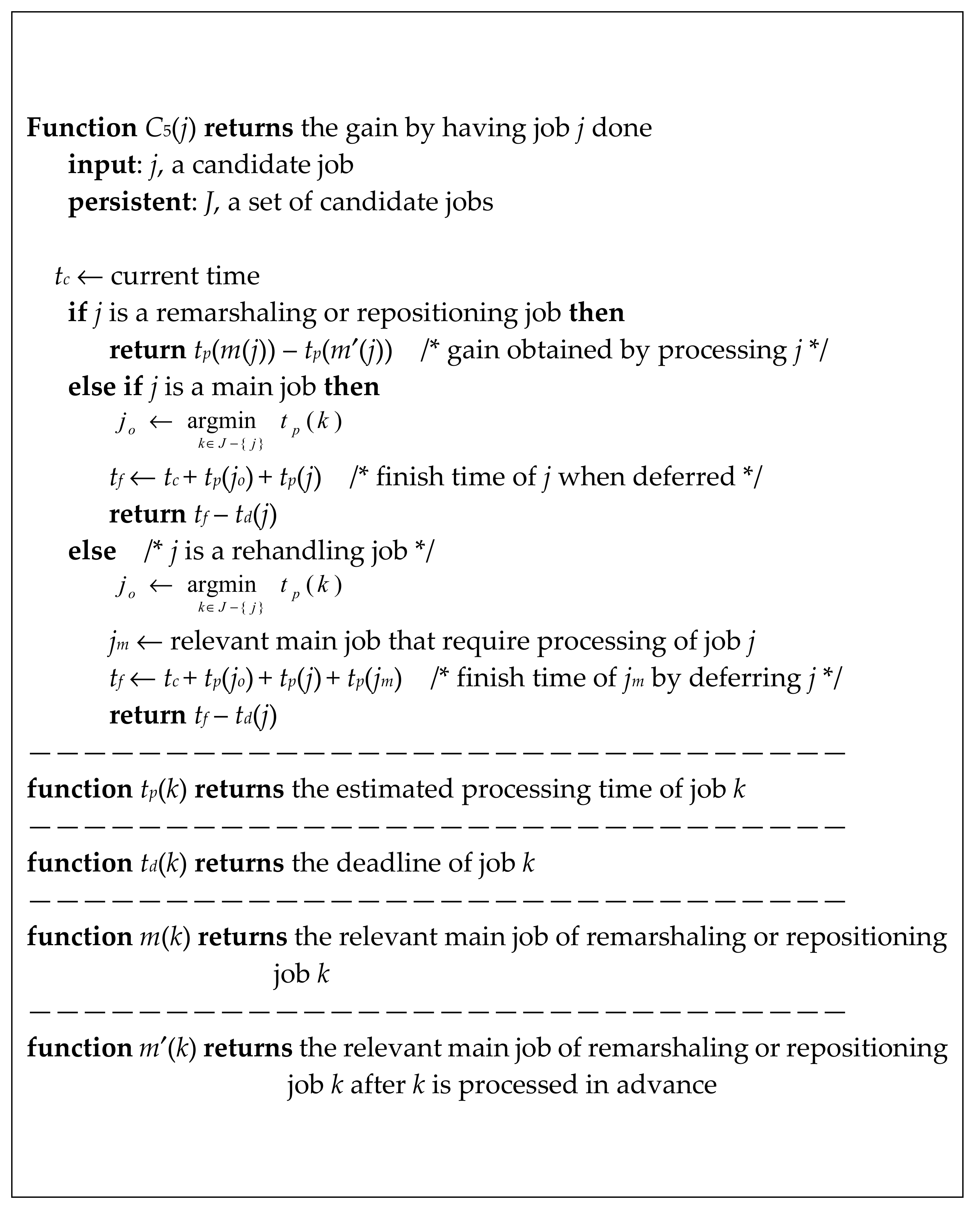
C5 estimates the gain obtained if the candidate job j under evaluation is done. Since a higher gain is preferable but the policy looks for a minimum score, the weight value for C5,when optimized, would be negative. If j is a remarshaling job, the gain is the amount of time to be saved at the time of loading (or carry-out) by having j done in advance. Let c be the container pertaining to the main job m(j), for which the remarshaling job j is prepared. Then, the remarshaling job j may involve either a relocation of c from its original location to a new location closer to its exit HP or a rehandling of a container stacked above c. In either scenario, j transforms its relevant main job from m(j) to m′(j). If the estimated amount of time needed to process a job k is denoted by tp(k), the gain obtained by performing the remarshaling job j can be estimated by tp(m(j)) − tp(m′(j)). The gain by a repositioning job can also be estimated in a similar way. However, since repositioning is usually more important (or urgent) than remarshaling and the seaside repositioning jobs are more important than the landside repositioning jobs, these job types are given different weights, as indicated by the different subscripts shown in Table 1. The gain obtained by doing a main job or rehandling job is computed from a quite different perspective because these jobs are not optional but mandatory. Choosing not to do such a job (j), at the current moment, only results in a postponement of j. Notice that postponing j is likely to lead to a delay. The larger the expected delay, the more important it is not to postpone j. Therefore, the gain by doing these jobs at the current moment can be considered to be the amount of expected delay caused by not doing them right away. To estimate the delay by a postponement, we optimistically assume that the job selected, instead of job j from the candidate job set J, is always the one with a minimum processing time. Figure 5 shows the pseudocode for calculating the criterion C5.
C6 is designed to promote load balancing between the two ASCs. It evaluates the degree of the relative advantage of having the job done by the other ASC, instead of the current ASC. The lower the evaluation value, the better the job is done by the current ASC than the other. If the job (j) under evaluation is a main job (i.e., seaside or landside job), the evaluation is zero because a main job cannot be processed by the other ASC. If j is a preparatory job (i.e., a rehandling or repositioning job) or a remarshaling job, the evaluation is made in the following way:
t p ( j ) i M t p ( i ) t p ( j ) k M t p ( k )
where tp(j) and tp(j) are the times taken to process job j by the current ASC and the other ASC, respectively, and M and M′ are the main jobs remaining in J to be done by the current ASC and the other ASC, respectively. This equation can be interpreted as the difference of the weighted processing times of the two ACSs, where each weight is the remaining workload of the respective ASC. When the remaining workloads of both ASCs are the same, job j is better done by the ASC with a shorter processing time. If the processing times of both ASCs are the same, the job is better done by the ASC with a lower remaining workload.
C7 estimates the waiting time due to interference with the other crane. The waiting time is 0 if no interference occurs when tested by simulation. If an interference occurs, the waiting time is the time taken until the other crane finishes its currently assigned job. This criterion discourages the selection of a job prone to ASC interference. C8 gives precedence to the main jobs by returning the evaluation value of zero for them. For the preparatory jobs, as well as the remarshaling jobs, a non-zero evaluation is made by multiplying the distance to the target stacking position (i.e., the distance of loaded travel by ASC) by the stacking density around the target position. A long distance to the target position means an inevitably long processing time. The stacking density around the target position is positively correlated with the ASC traffic in that area. Sending an ASC to a congested area is discouraged (to avoid crane interference). C9 is another maximizing criterion to promote a remarshaling job to be done only when the ASC workloads are low. If the candidate job is a main job or a preparatory job, the evaluation is zero. In the case of a remarshaling job, this criterion estimates the time remaining after all the main jobs and preparatory jobs within the scheduling horizon th are completed:
t h ( M + P ) × t ^ p
where t ^ p (assumed to be 100 s in this paper) is the average processing time needed by each job in M (set of main jobs remaining in J) or P (set of preparatory jobs remaining in J). C9 prefers a remarshaling job only when the value of Equation (5) is positive.

4.2. Objective Function

To optimize the crane dispatching policy, we used an evolutionary algorithm to search through the policy space. A candidate solution in this search is represented by a vector of weights. The crane dispatching policy has 17 weights (see Table 1), the values of which are constrained to be in the interval [−1, 1] in our search. To evaluate the performance of a candidate policy, we must simulate scenarios of crane operation at a block with the policy applied and observe the operational efficiency achieved. The objective function that we want to minimize is as follows:
f ( π d ) = W 1 D A G V ( π d ) + W 2 D E T ( π d )
where πd is the crane dispatching policy under evaluation, DAGV is the average (per container) AGV delay observed under πd, DET is the average waiting time of external trucks under πd, and W1 and W2 are the respective weights for DAGV and DET. Given a good policy, the cranes at a block work efficiently to process not only the main jobs but also the remarshaling jobs, thus minimizing the AGV delay and the ET waiting time in the long run. Since the seaside operations are considered much more important than the landside operations in most terminals, W1 is usually set to a much higher value than W2. For accurate evaluations of the policy, the search algorithm is provided with a set of simulation scenarios of operations at a block. The jobs in each scenario are randomly generated according to a realistic distribution based on the statistics of a real container terminal. The simulator that we use is event-driven and is the same as that described in [1]. It simulates the ASC operations in detail, including acceleration, deceleration, and their mutual interferences.

4.3. Noisy Optimization of Crane Dispatching Policy

The fitness evaluation of a candidate policy π through simulations of operation scenarios is subject to noise, due to the lack of the depth and breadth of the scenarios. Formally, a noisy fitness function g(π) can be expressed as follows:
g ( π ) = f ( π ) + z , z ~ N ( 0 , σ 2 )
where π is a candidate policy, f(π) is a noise-free fitness function, and z is the additive noise that is often assumed to be normally distributed with zero mean and variance σ 2. While the goal of optimization is to minimize f(π), only g(π) is observable during optimization. One practical way to approximate the real fitness is averaging the values of a sufficient number of fitness samples [28]:
f ( π ) 1 n i = 1 n g i ( π ) = 1 n i = 1 n f ( π ) + z i
where n is the number of samples and gi(π) is the ith estimate of the fitness.
In a noisy environment, the fitness comparison for the survival selection should be done probabilistically, considering the influence of noise. Assuming two independent random fitness value lists, x and y, the probability that x is better than y, p(yx), is calculated by using a Student’s t-distribution [11]:
p ( y x ) = F d ¯ / s d , v = d ¯ / s d f ( t , v ) d t
where the mean d ¯ = x ¯ y ¯ , σd is the standard deviation of d, and F is the cumulative distribution of the Student’s t-distribution f(t, ν) with ν degrees of freedom. σd and ν are calculated as follows:
σ d = x n 1 σ x 2 + y n 1 σ y 2 x n + y n 2
v = n x + n y 2
where xn and yn are the number of samples for x and y, respectively. Notice that the number of samples of the fitness of every newly born individual should be at least two for this probabilistic comparison, because otherwise, the variance becomes zero.
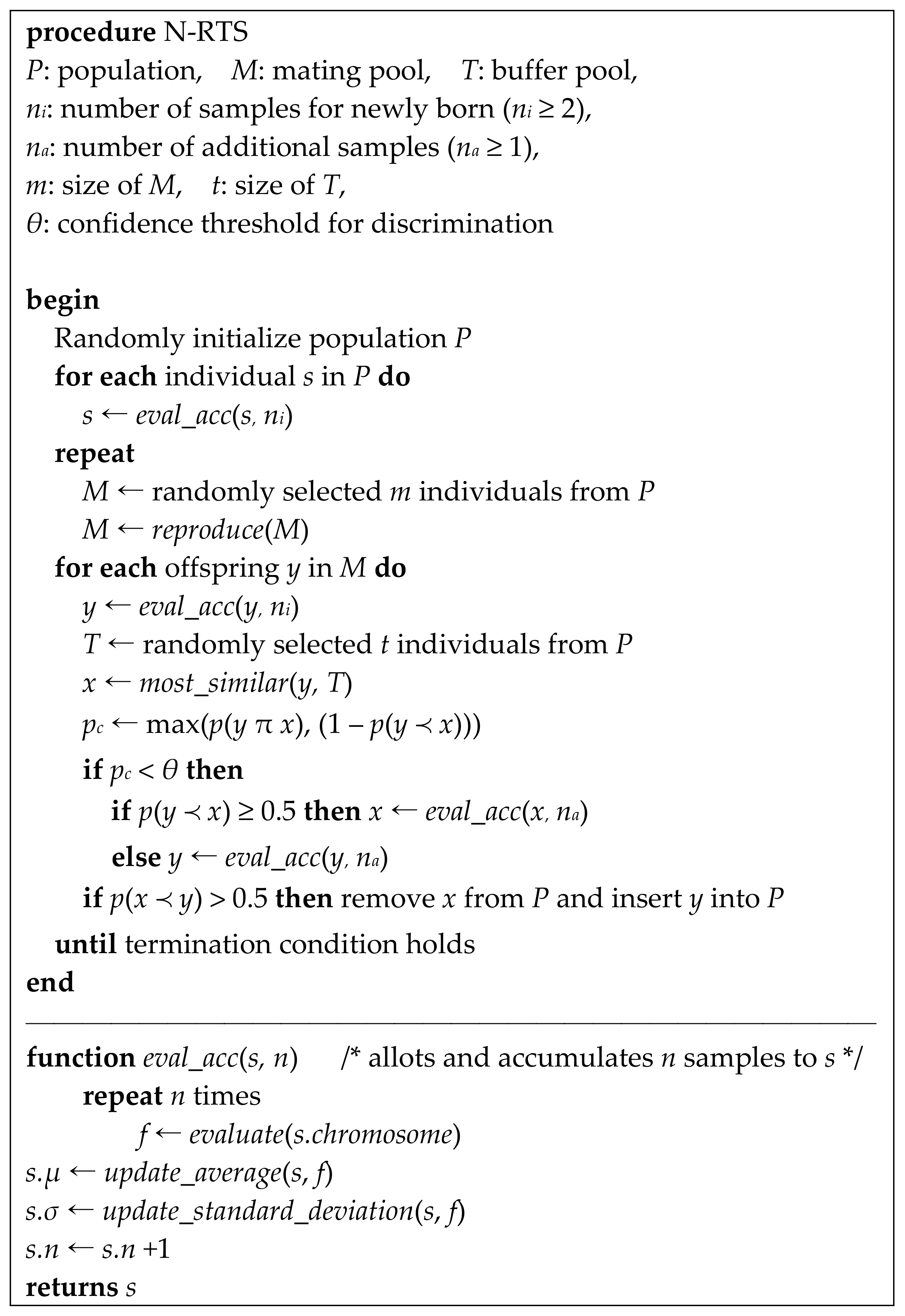
Figure 6 shows the pseudocode of N-RTS. The algorithm begins by initializing the population P with randomly generated policies (or weight vectors). Each policy is then evaluated by having ni (≥2) samples allotted to it, where each sample is the fitness value measured by simulating a scenario randomly picked from a large pool of scenarios. The evolutionary process consists of reproduction and survival selection steps that repeat until a termination condition holds. As it is one of the overlapping-generation models, parents and offspring compete with each other for survival. In the reproduction step, m individuals are randomly (with no regard to their fitness values) selected from P to form a mating pool M, from which the same number of offspring is generated by applying crossover and mutation operations. In the survival selection step that follows, each offspring y in M, after being evaluated with ni samples, competes with the individual x in P that is very similar to it. To find such an x, t individuals are randomly selected from P, and then the one most similar to y is identified. The similarity measure used is the Euclidean distance. In the original RTS, where there is no notion of noise, the one with higher fitness wins the survival selection and the loser is discarded. By discouraging similar individuals to reside together in the population, RTS avoids premature convergence by maintaining population diversity.
When the environment is noisy, however, the survival selection should be done not deterministically, but probabilistically. To determine the winner between the two individuals x and y, their sampled finesses are compared probabilistically by using Equation (9). We consider that x is probabilistically better than or equal to y if p(yx) ≥ 0.5, and vice versa if (1 − p(yx)) ≥ 0.5. The result of comparison pc = max(p(yx), (1 − p(yx))), therefore, is always greater than or equal to 0.5. If pc is close to 1, we believe x and y are significantly different, in which case we determine the winner without hesitation. If pc is smaller than a predetermined threshold θ, we try a more careful comparison by adopting the idea of accumulative sampling [11]. If the competitor x from P looks no worse than the newly born y (i.e., p(yx) ≥ 0.5), we give na additional samples to x and update its evaluation by averaging all the samples, including the additional samples and the existing ones. Otherwise, the additional samples are given to y and its evaluation is updated. The more samples allotted to an individual, the more reliable its evaluation becomes. The notable features of N-RTS are that it saves samples by giving additional samples only to a better looking one during the survival selection and no sample at all when one looks decisively better than the other, while NTGA unconditionally gives additional samples to x, regardless of the quality difference between x and y. The level of decisiveness can be controlled by adjusting the threshold value θ. As one wants a higher confidence for that decision, he or she needs a higher value of θ.
The sizes of P, T, and M were empirically set to 100, 50, and 2, respectively. The sizes of ni and na were set to 2 and 1, respectively. The binary tournament selection was used to form a mating pool (M) from the population (P). The confidence threshold θ was empirically set to 0.98. Each individual chromosome is represented as an array of real values. The crossover operator used is the simulated binary crossover [29], with a crossover rate of 0.9 and a crowding control parameter of 2. The mutation operator used is the polynomial mutation [29], with a mutation rate of 1/L (L is the length of the chromosome) and a crowding control parameter of 2.

5. Experimental Results

In this section, we tested the performance of the crane dispatching policy obtained by our policy search (PS) method (described in Section 4), in comparison to that of the online search (OnS) method by [5]. Our PS method attempted both NTGA and the newly proposed N-RTS to optimize (or to learn) the policy by simulating a set of training scenarios. The performance of the obtained policy was tested by applying it to a set of test scenarios through simulation and then measuring the average AGV delay and ET waiting time. The OnS method, instead of using a crane dispatching policy, repeatedly conducts a search to schedule the cranes to process the jobs in a horizon, but it also needs a policy for container stacking. The stacking policy for OnS is the one developed by [5], which is the same as that used by PS. The performance of OnS was also tested by using the same test scenarios as those used by PS, for a fair comparison. In addition, we conducted some additional experiments using a set of well-known benchmark functions to see how well N-RTS handles noise, compared to DS [8], MDE [24], and NTGA [12], when given various types of problems. Below, we begin by describing the simulation scenarios used for learning and testing, followed by the experimental setting. Then, we reported the results of simulation experiments and the test results with benchmark functions.

5.1. Simulation Scenarios

As shown in Table 2, the target block for our simulation experiments was 41 bays long, 10 rows wide, and 5 tiers high, which is a typically sized block seen in automated container terminals. A scenario consisted of jobs to be done for three weeks in this block, during which period 120 containers were discharged from a vessel, and the same number of containers were loaded onto the same vessel every day, with their due times randomly generated by following a uniform distribution. For simplicity, it was assumed that a new vessel was serviced every day, as the turnaround time of a vessel in real terminals is mostly less than 24 h. The proportion of the transshipment containers was 45%, which implies that there were much more seaside jobs than the landside jobs. This proportion of transshipment is the same as the average of the container terminals in Busan, Korea. Notice that the landside jobs (carry-in and carry-out jobs) and their due times were determined in accordance with the associated seaside jobs and their dwell times. More specifically, a container c1 discharged at time t1 was carried out of the block by an external truck at time t1 + d1, unless it was a transshipment container, where d1 was the dwell time of c1. Similarly, a non-transshipment container, c2, to be loaded at t2 was carried into the block at t2d2, where d2 was the dwell time of c2. A transshipment container, c3, discharged from a vessel at t3 was loaded onto another vessel at t3 + d3, where d3 was the dwell time of c3. The dwell time of each container was determined probabilistically by following the distribution used in [30], which is basically the same as the real distribution of a real terminal. A longer average dwell time leads to a higher block occupancy rate. In our experiment, the occupancy rate was adjusted to be around 60%. One hundred scenarios were randomly generated for training, as well as an additional set of ten scenarios for testing. The search algorithms were empirically set to terminate after 100,000 scenario simulations, taking a CPU time of approximately four and a half days on a PC with a 2 GHz CPU and 128 GB of RAM.
When searching for an optimal policy, each candidate policy was evaluated by a randomly selected training scenario with the candidate policy under enforcement and then measured its performance on that scenario. The first two weeks of the three-week simulation was an initialization period, during which time containers came into an initially empty block and were stacked there, while some of them were retrieved after their dwelling periods. All these container movements during this initialization period were made without any crane scheduling and simulation (to save the CPU time). While the stacking positions of the incoming containers were determined by the stacking policy by [5], the dispatching policy was not used during the initialization because there was no crane scheduling. Instead, the jobs were simply processed in the order of their due times and neither repositioning nor remarshaling was performed. When a container stacked under some others needed to be retrieved, it was taken directly out, with the heights of those above it lowered by one tier. The processing of the jobs of the third week was simulated with the policies under enforcement. The cranes were scheduled by being dispatched using the dispatching policy, and the crane movements were realistically simulated depicting their accelerations, decelerations, and mutual interferences by using the simulator developed by [1]. All types of jobs, including rehandling, repositioning, and remarshaling were done. It was during this third week that the average AGV delay and ET waiting time were measured as the performance indicator of the policy under evaluation. Once an optimal policy was obtained, the ten test scenarios were used to measure the performance of the policy. The simulation of the test scenarios was conducted in exactly the same way as that of the training scenarios.

5.2. Experimental Setting

OnS [5] uses a genetic algorithm to search for a good crane schedule for the jobs in a horizon. The length of horizon and the rescheduling interval were set to 30 and 15 min, respectively, as chosen by [5]. Since not much time (less than 15 min) was allowed for the search (for rescheduling), their genetic algorithm terminated after 800 evaluations of the candidate crane schedules. PS conducts crane scheduling by using its dispatching policy without any search involved. To recommend a job to be done next by an ASC, the policy evaluates all the candidate jobs for the ASC within a scheduling horizon and selects the best one (Figure 4 in Section 4). The longer the horizon, the more candidate jobs there are to select from. Its length was empirically set to 60 min (Explained in Section 5.3). PS reschedules for the cranes whenever an ASC completes its job, as dispatching takes a very small amount of computation time. The ratio of the weights to the two objectives, i.e., AGV delay and ET waiting time, was also determined empirically as 300:1 for OnS and 100:1 for PS (Explained in Section 5.3). All these settings were used not only for testing but also for training. Table 3, below, summarizes these settings.

5.3. Performance Comparison

Table 4 shows the results of the experiments, comparing the performances of PS by N-RTS, PS by NTGA, and OnS. Since the evolutionary algorithms are stochastic, the policies resulting from different search sessions are different, showing different performances. Therefore, we collected ten dispatching polices by running N-RTS ten times and another ten by running NTGA ten times. Then, the performance of PS by N-RTS, for example, on a test scenario, was obtained by applying each of the ten policies to the scenario and averaging the observed performances. To make our performance comparison more reliable, we used ten test scenarios and compared the test results by using a non-paired t-test with a significance level of 0.95. Notice that every number in Table 4 is, thus, an average of one hundred numbers. We can see that PS by N-RTS clearly dominates not only PS by NTGA but also OnS in terms of both AGV delay and ET waiting time. Another important advantage of using the dispatching policy is that it can be applied with a very small amount of computational overhead. Applying OnS to a single test scenario takes a CPU time of longer than one and a half days, in contrast to less than a few seconds in the cases of applying the policy. After some calculations, we roughly estimated that applying OnS to a real terminal with 22 storage blocks, for example, would require more than three dedicated CPUs.
While PS can reschedule almost immediately after each job, OnS cannot afford to do this, due to the heavy computational overhead. The shorter the rescheduling interval, the less likely it becomes that the result of the schedule execution deviates from the expected outcome in an uncertain environment where the operations of ETs, AGVs, and cranes are not deterministic. Another advantage of PS is that it allows a longer scheduling horizon than OnS (Table 3), due to the small computational overhead of applying the policy. However, longer horizons are not always better. Table 5 shows the effects of horizon length on the search for a dispatching policy by N-RTS. The table also shows the effects of different combinations of objective weights. The policies are learned from the same training scenarios as those used in the above experiments (Table 4). The test results given in Table 5 were obtained by applying the policies to ten separately generated test scenarios. The AGV delay and ET waiting times are the average results of applying ten policies, obtained by running N-RTS ten times. Increasing the horizon length from 30 to 60 min resulted in an overall performance improvement, regardless of the objective weight combination. However, a further increase leads to a deterioration in performance. Regarding the objective weight combinations, we see that a hundred times higher weight to AGV than to ET gives rise to the best performance. The performance degrades when the weight to AGV is either too high or too low.

5.4. Test Results with Benchmark Functions

To see how well N-RTS handles noisy optimization problems, compared to other noisy optimization methods, we conducted additional experiments with some benchmark functions used in the study of [15], as listed in Table 6 (the dimensionality was set to 30). We generated three noisy test cases from each of these functions by adding zero-mean Gaussian noise, with the standard deviation corresponding to 5%, 10%, and 20% of its codomain range R, respectively. The codomain range R of a function was estimated by calculating the difference between the average of the function values of 100 points randomly generated within the decision space and the optimal (i.e., the minimum) value. For each test case, algorithms to be compared were run 50 times, and their results were averaged. The total number of evaluations (i.e., samples) was fixed to 100,000 and the other parameter settings were the same as those described previously. After each run of an algorithm, the individual with the best sampled evaluation was picked up from the population, and then its noise-free actual value was identified. This actual value was treated as the solution that the algorithm had found. Table 7 shows the results of non-paired t-tests with a confidence level of 95%, comparing N-RTS against RTS, NTGA, DS, and MDE. Since RTS is not equipped with any noise handling scheme, it adopts the simple resampling strategy, according to which each individual is evaluated, by giving a sufficient number of samples. The number of samples in our experiment was set to 5, which is empirically shown to achieve the best balance between exploration and exploitation. The parameters of DS and MDE were set to the same values as those chosen by [3]. The values under the column heading σ are the noise levels tested. Additionally, ‘+’ indicates that N-RTS performs significantly better than the respective algorithm listed in the leftmost column of the same row and ‘=’ indicates that the performances of the compared algorithms cannot be considered significantly different. As can be seen in the table, the performance of N-RTS easily dominates RTS, DS, and MDE and is better than, or at least similar to, NTGA.
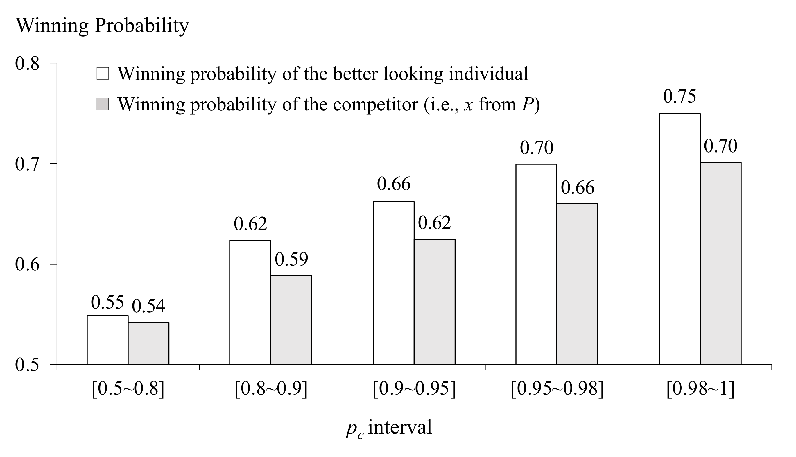
Figure 7 shows the distribution of the probability values observed at the probabilistic comparison step (i.e., the observed values of pc in the pseudocode of Figure 6) during the search for an optimal solution of the Ackley function (σ = 0.1) by N-RTS. The cases with a probability lower than 0.8 account for 46% of the total, for which the comparison results are not considered decisive. Since the confidence threshold θ was set to 0.98 in N-RTS, 11% of the total cases were considered decisive, for which no additional samples were needed to identify the winner. The samples saved in this way contributed to examining more unexplored candidates in the search space, thus enhancing the search performance. Figure 8 summarizes another analysis result of the logs of the survival selection step of N-RTS during the optimization of the Ackley function (σ = 0.1). Recall that the individuals involved in the survival selection were a newly born y and a competitor x, chosen from the population (Figure 6). While N-RTS gives additional samples to the better-looking one among x and y only when the judgement is not decisive, NTGA unconditionally gives additional samples to x. The white bars in Figure 8 show the probabilities that the better-looking one is really a winner (when judged by noise-free fitness). We can see that this probability increases as the value of pc (confidence of comparison) increases. The shaded bars in the figure show the probabilities that x (the one NTGA chooses) is a real winner, which are consistently lower than the white bars. The additional samples invested in the losers were dumped and not accumulated, to contribute to making the evaluations more reliable. What would happen if θ is lowered to, for example, 0.95? Figure 7 shows that additional samples can be saved for up to 21% of the survival selection cases. The cost that we pay for this is that the real winning probability of the better-looking individual can be reduced to 0.70 from 0.75, as indicated in Figure 8. Additionally, θ must be determined carefully, considering this tradeoff.

6. Conclusions

In this paper, we proposed using a crane dispatching policy to schedule the ASCs at the storage block of an automated container terminal. We also proposed a noisy optimization algorithm, named N-RTS, that can efficiently search for a good dispatching policy. Simulation experiments showed that our dispatching policy outperformed the online search method (OnS) by [5], in terms of both the quality of the crane schedules and the CPU times taken to derive the schedules.
It has been generally suspected that deriving crane schedules of higher quality than those by OnS would be difficult, as the outcome of OnS is the result of an optimization search obtained through the significant investment of computational resources. The surprising success of the policy seems to be due to two reasons. First, the policy is not myopic (as are other simple heuristics), as it is optimized through simulations of long and diverse operation scenarios. Second, the scheduling horizon used by the policy is twice as long as that used by OnS (60 vs. 30 min). While OnS cannot afford to have a long horizon, as its optimization has to be completed in real time, the policy is free from such concern as it takes a small amount of time to build a schedule, given a long horizon.
While our policy was very powerful and quick in usage, it was computationally demanding to search for a good policy, due to the heavy simulations involved. N-RTS makes this search efficient by smartly allotting samples to individuals for evaluation. Experiments with some benchmark functions revealed that 11% of all the competitions for survival selection, in which one looked obviously better than the others, were processed without using any additional samples. This savings contributed to enhanced search performance, by being invested in exploring more individuals in the search space. For the remaining cases, where the comparison results were not decisive, N-RTS invested additional samples in the better-looking individuals, to make their evaluations more reliable. This strategy turned out to be better than that adopted by NTGA, where the additional samples were never given to the newly born, but only to the old competitor from the population. Since the better-looking individual is more likely to win the survival selection, as seen from the last experiment, the samples invested in them are more likely to be accumulated to contribute to more reliable evaluations later. When the optimization problem at hand requires heavy simulations during the search, N-RTS would be a useful tool to find a solution effectively and efficiently.

Author Contributions

Conceptualization, J.K. and K.R.R.; methodology, J.K., E.J.H., Y.Y. and K.R.R.; software, J.K.; validation, J.K. and K.R.R.; formal analysis, J.K and K.R.R.; investigation, J.K. and K.R.R.; resources, J.K.; data curation, J.K. and K.R.R.; writing—original draft preparation, J.K.; writing—review and editing, K.R.R.; visualization, J.K.; supervision, K.R.R.; project administration, K.R.R.; funding acquisition, K.R.R. All authors have read and agreed to the published version of the manuscript.

Funding

This work was supported by Institute of Information & Communications Technology Planning & Evaluation (IITP) grant, funded by the Korea government (MSIT) (No. 2020-0-01450, Artificial Intelligence Convergence Research Center [Pusan National University]).

Institutional Review Board Statement

Ethical review and approval were waived for this study, since no experimentation was carried out on human beings. The involvement of humans was limited to the completion of a questionnaire, for which informed consent was regularly obtained.

Informed Consent Statement

Informed consent was obtained from all subjects involved in the study.

Data Availability Statement

Data sharing is not applicable to this article.

Conflicts of Interest

The authors declare no conflict of interest.

References

  1. Park, T.; Choe, R.; Ok, S.M.; Ryu, K.R. Real-time scheduling for twin RMGs in an automated container yard. OR Spectr. 2010, 32, 593–615. [Google Scholar] [CrossRef]
  2. Ng, W.C.; Mak, K.L. Yard crane scheduling in port container terminals. Appl. Math. Model. 2005, 29, 263–276. [Google Scholar] [CrossRef] [Green Version]
  3. Li, W.; Wu, Y.; Petering, M.E.H.; Goh, M.; de Souza, R. Discrete time model and algorithms for container yard crane scheduling. Eur. J. Oper. Res. 2009, 198, 165–172. [Google Scholar] [CrossRef] [Green Version]
  4. He, J.; Chang, D.; Mi, W.; Yan, W. A hybrid parallel genetic algorithm for yard crane scheduling. Transp. Res. Part E Logist. Transp. Rev. 2010, 46, 136–155. [Google Scholar] [CrossRef]
  5. Choe, R.; Kim, T.S.; Kim, T.; Ryu, K.R. Crane scheduling for opportunistic remarshaling of containers in an automated stacking yard. Flex. Serv. Manuf. J. 2015, 27, 331–349. [Google Scholar] [CrossRef]
  6. Hu, Z.H.; Sheu, J.B.; Luo, J.X. Sequencing twin automated stacking cranes in a block at automated container terminal. Transp. Res. Part C Emerg. Technol. 2016, 69, 208–227. [Google Scholar] [CrossRef]
  7. Jiang, X.J.; Jin, J.G. A branch-and-price method for integrated yard crane deployment and container allocation in transshipment yards. Transp. Res. Part B Methodol. 2017, 98, 62–75. [Google Scholar] [CrossRef]
  8. Aizawa, A.N.; Wah, B.W. Scheduling of Genetic Algorithms in a Noisy Environment. Evol. Comput. 1994, 2, 97–122. [Google Scholar] [CrossRef]
  9. Di Pietro, A. Optimising Evolutionary Strategies for Problems with Varying Noise Strength; The University of Western Australia: Perth, Australia, 2007. [Google Scholar]
  10. Zhang, Z.; Xin, T. Immune Algorithm with Adaptive Sampling in Noisy Environments and Its Application to Stochastic Optimization Problems. IEEE Comput. Intell. Mag. 2007, 2, 29–40. [Google Scholar] [CrossRef]
  11. Park, T.; Ryu, K.R. Accumulative sampling for noisy evolutionary multi-objective optimization. In Proceedings of the 13th Annual Conference on Genetic and Evolutionary Computation—GECCO’11, Dublin, Ireland, 12–16 July 2011; ACM Press: New York, NY, USA, 2011; pp. 793–800. [Google Scholar]
  12. Jang, H.; Choe, R.; Ryu, K.R. Deriving a robust policy for container stacking using a noise-tolerant genetic algorithm. In Proceedings of the 2012 ACM Research in Applied Computation Symposium on—RACS’12, San Antonio, TX, USA, 23–26 October 2012; ACM Press: New York, NY, USA, 2012; p. 31. [Google Scholar] [CrossRef]
  13. Fieldsend, J.E.; Everson, R.M. The Rolling Tide Evolutionary Algorithm: A Multiobjective Optimizer for Noisy Optimization Problems. IEEE Trans. Evol. Comput. 2015, 19, 103–117. [Google Scholar] [CrossRef]
  14. Hong, J.H.; Ryu, K.R. Simulation-based multimodal optimization of decoy system design using an archived noise-tolerant genetic algorithm. Eng. Appl. Artif. Intell. 2017, 65, 230–239. [Google Scholar] [CrossRef]
  15. Choe, R.; Jang, H.; Ryu, K.R. Deriving a Robust Policy for Container Stacking Using a Noise-Tolerant Genetic Algorithm. Information 2013, 16, 6219–6242. [Google Scholar]
  16. Kim, J.; Ryu, K.R. An RTS-based algorithm for noisy optimization by strategic sample accumulation. In Proceedings of the 2020 Genetic and Evolutionary Computation Conference Companion, Cancún, Mexico, 8–12 July 2020; ACM: New York, NY, USA, 2020; pp. 45–46. [Google Scholar]
  17. Kim, T.; Yang, Y.; Bae, A.; Ryu, K.R. Optimization of Dispatching Strategies for Stacking Cranes including Remarshaling Jobs. J. Navig. Port Res. 2014, 38, 155–162. [Google Scholar] [CrossRef] [Green Version]
  18. Briskorn, D.; Emde, S.; Boysen, N. Cooperative twin-crane scheduling. Discret. Appl. Math. 2016, 211, 40–57. [Google Scholar] [CrossRef]
  19. Gharehgozli, A.H.; Laporte, G.; Yu, Y.; de Koster, R. Scheduling Twin Yard Cranes in a Container Block. Transp. Sci. 2015, 49, 686–705. [Google Scholar] [CrossRef] [Green Version]
  20. Hirashima, Y.; Takeda, K.; Harada, S.; Deng, M.; Inoue, A. A Q-Learning for Group-Based Plan of Container Transfer Scheduling. JSME Int. J. Ser. C 2006, 49, 473–479. [Google Scholar] [CrossRef] [Green Version]
  21. Kang, J.; Oh, M.-S.; Ahn, E.Y.; Ryu, K.R.; Kim, K.H. Planning for Intra-block Remarshalling in a Container Terminal. In Advances in Applied Artificial Intelligence; Springer: Berlin/Heidelberg, Germany, 2006; pp. 1211–1220. [Google Scholar] [CrossRef]
  22. Park, K.; Park, T.; Ryu, K.R. Planning for Selective Remarshaling in an Automated Container Terminal Using Coevolutionary Algorithms. Int. J. Ind. Eng. Theory Appl. Pract. 2013, 20, 176–187. [Google Scholar]
  23. Di Pietro, A.; While, L.; Barone, L. Applying evolutionary algorithms to problems with noisy, time-consuming fitness functions. In Proceedings of the 2004 Congress on Evolutionary Computation (IEEE Cat. No.04TH8753), Portland, OR, USA, 19–23 June 2004; pp. 1254–1261. [Google Scholar]
  24. Mininno, E.; Neri, F. A memetic Differential Evolution approach in noisy optimization. Memetic Comput. 2010, 2, 111–135. [Google Scholar] [CrossRef]
  25. Siegmund, F.; Ng, A.H.C.; Deb, K. A comparative study of dynamic resampling strategies for guided Evolutionary Multi-objective Optimization. In Proceedings of the 2013 IEEE Congress on Evolutionary Computation, CEC 2013, Cancun, Mexico, 20–23 June 2013. [Google Scholar]
  26. Harik, G.R. Finding Multimodal Solutions Using Restricted Tournament Selection. In Proceedings of the 6th International Conference on Genetic Algorithms, San Francisco, CA, USA, 15–19 July 1995; Morgan Kaufmann Publishers Inc.: San Francisco, CA, USA, 1995; pp. 24–31. [Google Scholar]
  27. Park, T.; Sohn, M.; Ryu, K.R. Optimizing stacking policies using an MOEA for an automated container terminal. In Proceedings of the 40th International Conference on Computers & Indutrial Engineering, Awaji, Japan, 25–28 July 2010; pp. 1–6. [Google Scholar]
  28. Jin, Y.; Branke, J. Evolutionary Optimization in Uncertain Environments—A Survey. IEEE Trans. Evol. Comput. 2005, 9, 303–317. [Google Scholar] [CrossRef] [Green Version]
  29. Yu, X.; Gen, M. Introduction to Evolutionary Algorithms; Decision Engineering; Springer: London, UK, 2010; ISBN 978-1-84996-128-8. [Google Scholar]
  30. Park, T.; Choe, R.; Hun Kim, Y.; Ryel Ryu, K. Dynamic adjustment of container stacking policy in an automated container terminal. Int. J. Prod. Econ. 2011, 133, 385–392. [Google Scholar] [CrossRef]
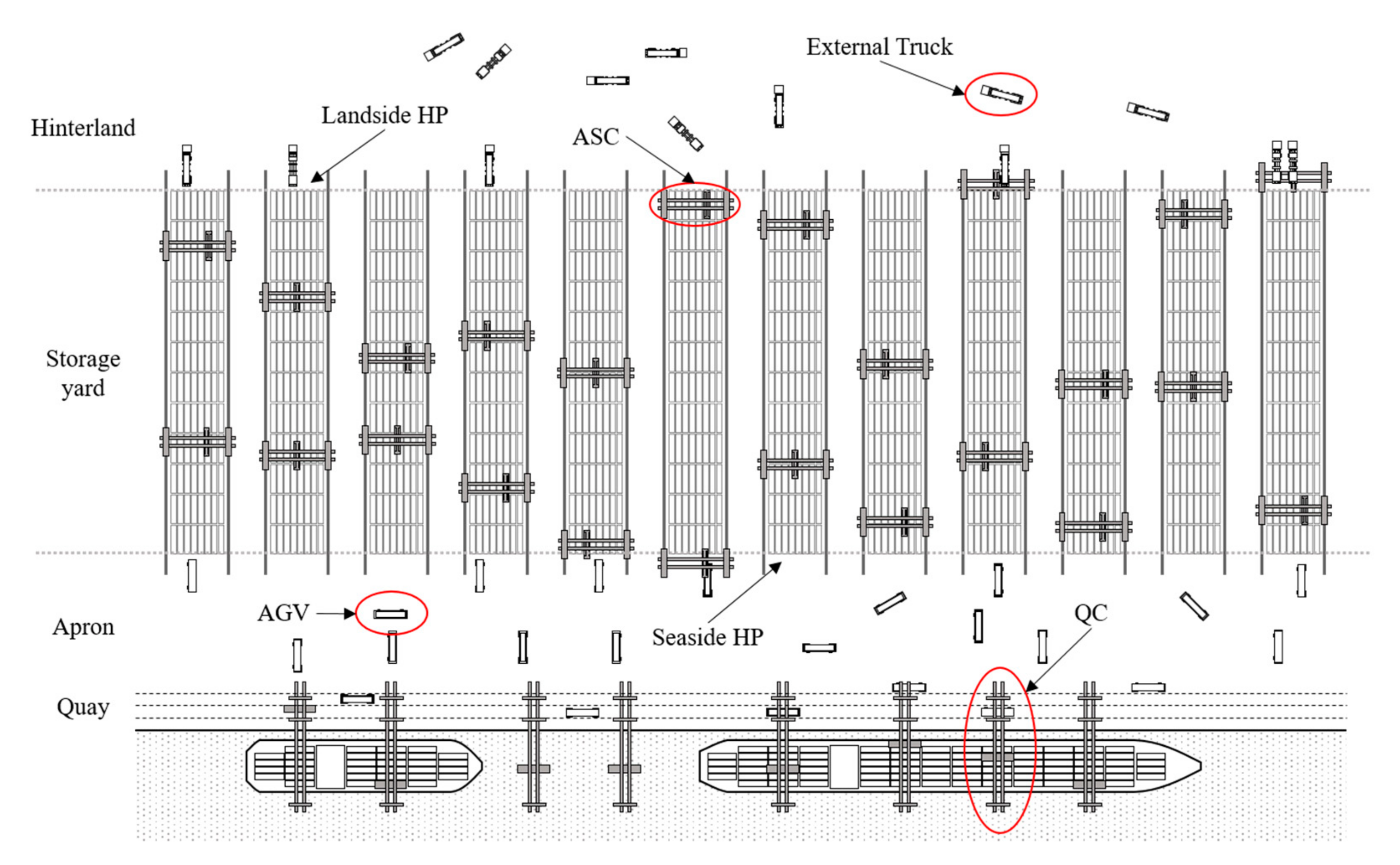
Figure 1. Layout of an automated container terminal (adapted from [5]).
Applsci 11 06922 g001
Figure 2. Structure of a storage block (adapted from [12]).
Applsci 11 06922 g002
Figure 3. Structure of a storage block (adapted from [17]).
Applsci 11 06922 g003
Figure 4. Procedure of ASC operations at a yard block using the stacking and dispatching policies.
Applsci 11 06922 g004
Figure 5. Pseudocode for evaluating the criterion C5.
Applsci 11 06922 g005
Figure 6. Pseudocode of N-RTS.
Applsci 11 06922 g006
Figure 7. Distribution of the values of pc during the search for an optimal solution of the Ackley function (σ = 0.1) by N-RTS.
Applsci 11 06922 g007
Figure 8. The winning probabilities of chosen individuals at different values of pc during the search for an optimal solution of the Ackley function (σ = 0.1) by N-RTS.
Applsci 11 06922 g008
Table 1. Evaluation criteria for different job types for the crane dispatching policy.
DescriptionCriterionRelevant Job Type
Empty travel distanceC1All types
Margin to due timeC2,aSeaside job
Seaside rehandling job
Seaside repositioning job
C2,bLandside job
Landside rehandling job
Landside repositioning job
C2,cRemarshaling job
Probability of ASC interferenceC3All types
Estimated processing timeC4All types
Gain by doing the current jobC5,dSeaside job
C5,eSeaside rehandling job
C5,fSeaside repositioning job
C5,gLandside job
C5,hLandside rehandling job
C5,iLandside repositioning job
C5,jRemarshaling job
Advantage if done by the other ASCC6All types
Waiting time by ASC interferenceC7All types
Job priorityC8All types
Time available for remarshalingC9All types
Table 2. Setting for simulation scenarios.
ParameterValue
Block size41 bays, 10 rows, 5 tiers
Duration of simulation14 days of initialization + 7 days of evaluation
Discharging jobs per day120 containers
Loading jobs per day120 containers
Proportion of transshipment jobs45%
Average occupancy rate60%
Table 3. Setting for the experiments.
OnSPS
Length of horizon30 min.60 min.
Rescheduling interval15 min.After each job
No. of evaluations for search800/rescheduling-
Weights for objectives300: 1100: 1
Table 4. Results obtained by averaging the performances measured on ten test scenarios (significance level: 0.95).
PS by N-RTSPS by NTGAOnS
AGV delay (sec)16.9 ± 1.218.7 ± 0.819.3 ± 2.1
ET waiting (sec)293.6 ± 59.6370.2 ± 71.7771.8 ± 69.7
t-test (AGV delay)NTGA, OnS--
t-test (ET waiting)NTGA, OnSOnS-
Table 5. Performance of PS by N-RTS with different values of objective weight and horizon length.
Horizon Length
(min)
Objective Weights
(AGV Delay: ET Waiting)
AGV Delay
(sec)
ET Waiting
(sec)
3050: 121.4 ± 1.9550.3 ± 112.3
100: 126.4 ± 2.3782.5 ± 135.2
300: 120.4 ± 2.4547.7 ± 89.4
500: 124.1 ± 2.5813.5 ± 90.2
6050: 123.5 ± 1.8284.4 ± 82.1
100: 116.8 ± 1.4298.2 ± 62.4
300: 117.5 ± 2.3287.3 ± 72.3
500: 124.4 ± 2.6361.5 ± 100.2
9050: 118.5 ± 2.9346.3 ± 130.7
100: 121.6 ± 3.1338.5 ± 149.1
300: 121.3 ± 2.2357.9 ± 101.2
500: 128.8 ± 2.2366.5 ± 200.6
Table 6. Benchmark functions used for testing noise handling performance.
FunctionDecision Space
Ackley 20 20 exp 0.2 1 n i = 1 n x i 2 + e exp 1 n i = 1 n cos 2 π x i [−1, 1]n
Alpine i = 1 n x i sin x i + 0.1 x i [−10, 10]n
Axis-parallel i = 1 n i x i 2 [−5.12, 5.12]n
DeJong x 2 [−5.12, 5.12]n
Drop wave 1 + cos ( 12 x 2 ) 1 2 x 2 + 2 [−5.12, 5.12]n
Table 7. Results of non-paired t-tests with a confidence level of 95%, comparing N-RTS against other algorithms by using the benchmark functions of Table 6 with different noise levels.
σAckleyAlpineAxis
Parallel
DeJongDrop Wave
RTS5%+++++
10%+++++
20%+++++
NTGA5%++===
10%++===
20%=+===
DS5%+++++
10%+++++
20%+++++
MDE5%++++=
10%+++++
20%+++++
Publisher’s Note: MDPI stays neutral with regard to jurisdictional claims in published maps and institutional affiliations.