Three-Dimensional Numerical Investigations of the Flow Pattern and Evolution of the Horseshoe Vortex at a Circular Pier during the Development of a Scour Hole

Featured Application

The (k-ω) turbulence model showed good results in capturing the flow structure at the wake zone downstream of the pier, with continuous oscillation matching the pier downstream turbulence pattern. Personal computer computational and storage resources were sufficient to run the computational fluid dynamics (CFD) simulations for the case in hand with the selected turbulence model. The required computational resources are cheap and affordable compared to those required for the Large Eddy Simulation (LES) and Detached Eddy Simulation (DES). This will lead to significant savings in time and resources in future CFD modeling for similar cases.

Abstract

In the current study, a three-dimensional CFD model is utilized to investigate the variation of the flow structure and bed shear stress at a single cylindrical pier during scour development. The scour development is presented by seven solidified geometries of the scour hole, collected during previous experimental work at different scour stages. Different turbulence models are evaluated and the (k-ω) model is chosen due to its relative accuracy in capturing the flow oscillation and vortex shedding at the pier downstream side with personal computer computational and storage resources. The numerical results are verified against dimensionless parameters from different previous experimental works. This research describes in detail the flow structure and bed shear stress variations through seven stages of the scour hole development. The dimensionless area-averaged circulation coefficient (Ψ_i) is developed to evaluate the changes in the vortex strength through the scouring process by eliminating the calculation area effect. It was concluded that the circulation in the (Y) direction is the main driving factor in the development of the scour hole more than the circulation in the (X) direction. The ratio between the horseshoe vortex (HV) mean size and the scouring depth (D_V/d_S) in addition to the location of the maximum bed shear stress are investigated during different stages of the scour development.

1. Introduction

The majority of bridge failure incidents are caused by the scour phenomenon at bridge pier foundations. The level and the type of bridge pier foundations are directly related to the scour depth that has a significant impact on the bridge’s construction cost. A better understanding of the flow structure and the bed shear stress distribution around bridge piers will enhance the prediction of the scour depth, and consequently will reduce the bridge construction cost.

In numerical modeling simulations of the flow structure around piers, no agreement among researchers has been achieved regarding the appropriate turbulence model for the numerical simulation. Additionally, most of the previous flow structure numerical simulations have been carried out using rigid flat bed and/or solidified equilibrium scoured bed geometries. Numerous laboratory studies have been carried out to develop equations to predict the maximum scour depth [1,2,3,4,5,6,7,8,9]. The available experimentally developed scour equations have been investigated and were found to over predict the scour depth, especially for skewed, long, and wide piers [10]. In subcritical flow conditions where the Froude number < 1, the maximum ratio between the equilibrium scour depth and the pier diameter (d_se/D) was experimentally obtained around 2.4 [11]. Other experiments under supercritical flow conditions revealed that (d_se/D) reached 3.0 at a Froude number = 1.5 [4].

The development of local scour at bridge piers is directly affected by the flow field structure around the pier and near the bed where downward flow, HV, and wake vortices are generated. The stream velocity decelerates while approaching the pier until it reaches stagnation at the pier’s upstream side face. The generated stagnation pressure gradient between the water surface and the bed at the pier’s upstream face generates a downward flow [12]. The generated downward flow acts as a vertical jet, which plays a significant role in the erosion of the bed material and the formation of the scour hole [13]. It has been claimed that the HV is a consequence of scouring, not the cause of it [12]. Therefore, a better understanding of the dynamic interaction between the flow field and the scouring process is still a pressing need to accurately simulate and predict the scour depth.

Several researchers have conducted experimental investigations of the flow field structure through the development of scour holes around piers [14,15,16,17,18,19,20,21]. The scour hole is initiated by two small scour holes at $\pm {100}^{°}$to the flow direction. They then move around the pier perimeter and merge at the pier’s upstream side along the stream centerline [14]. The maximum magnitude of the downward velocity (V) in front of the pier has a wide range of reported values relative to the depth-averaged approach velocity (U_o). The values varied between (−0.47 U_o) [18], (−0.60 U_o) [16,17,19], (−0.80 U_o) [14], and (−0.95 U_o) [15].

The development of CFD models motivated the use of numerical simulations [22,23,24,25,26]. No agreement among researchers has been achieved regarding the appropriate turbulence model for the numerical simulation of the flow structures and the bed shear stress around the bridge piers. The (k-ε) model was recommended by the authors of [27,28,29], while the (k-ω) was recommended by the authors of [30,31], and the Reynolds Stress Model (RSM) was found to provide satisfactory results [32]. The (k-ε) and the (RNG k-ε) turbulence models provide identical results for bed shear stress [33].

The increase in computational and digital storage capacities has led to an increase in LES and DES models. LES and DES have proved adequate in simulating large scale coherent eddies around piers [34,35]. The pier Reynolds number (R_eD) is calculated based on the pier diameter (D) and the depth-averaged approach velocity (U_o). The DES was used for piers with a high pier Reynolds number, which lies outside the range of well-resolved LES [36,37]. The DES is also used for rectangular piers with a high aspect ratio. The obtained results showed high bed shear stress values extended for a distance ranged between a 6 and 8 pier width upstream from the pier. Moreover, the nondimensional pressure root-mean-square (RMS) fluctuations at the bed were one order of magnitude higher than the simulated ones for circular piers [38]. The LES captured bimodal random oscillations in the necklace vortices forming the horseshoe system during all scour stages [36,37]. It was concluded that the flow remains subcritical near the bed surface due to the reduction in the boundary layer, for both a high and low pier Reynolds number [39].

The sub-particle-scale (SPS) turbulence closure scheme was used in the three-dimensional Incompressible Smoothed Particle Hydrodynamics (ISPH) erosion model to account for turbulence scales that are below the sediment particle size. The three-dimensional ISPH model was utilized to simulate the local scour at a relatively large cylindrical pier by using the turbidity water particle concept (TWP). The obtained scour hole depths had a suitable degree of accuracy for engineering purposes in some cases, and significant errors in other cases. It was concluded that obtaining a highly reliable scouring effect is very difficult even with experimental studies [40]. The eddy viscosity and turbulent shear stress were estimated by applying the SPS turbulence model with the Smagorinsky approach. The accurate investigation of the SPS turbulence closure scheme especially at the interfacial boundaries was not possible due to the lack of detailed turbulence data [41]. The continuous improvement in turbulence modeling, especially within the roughness layer in the macroscopic simulation of rough boundaries, will enhance the CFD modeling for the bed shear stress and accordingly, the sediment initiation of motion. A proposed three layer mixing length model was developed to represent the eddy structure sizes in the porous bed, the roughness layer, and the free flow zones in the case of channel flows over and within natural porous beds [42].

In short, CFD techniques are beneficial tools to understand the complexity of flow fields around bridge piers. Despite some successful scour modeling attempts, CFD techniques are characterized by their limited ability to simulate scour and erosion processes; as a result, their fidelity in scour depth estimation is limited [43].

The two main objectives of the current research are:

• Selecting an appropriate turbulence model with personal computer computational resources that can simulate the case in hand with acceptable accuracy, since no agreement between researchers has been achieved yet;
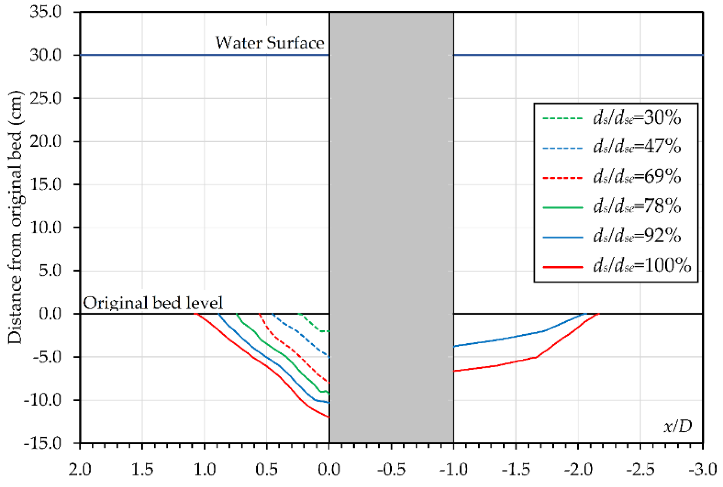
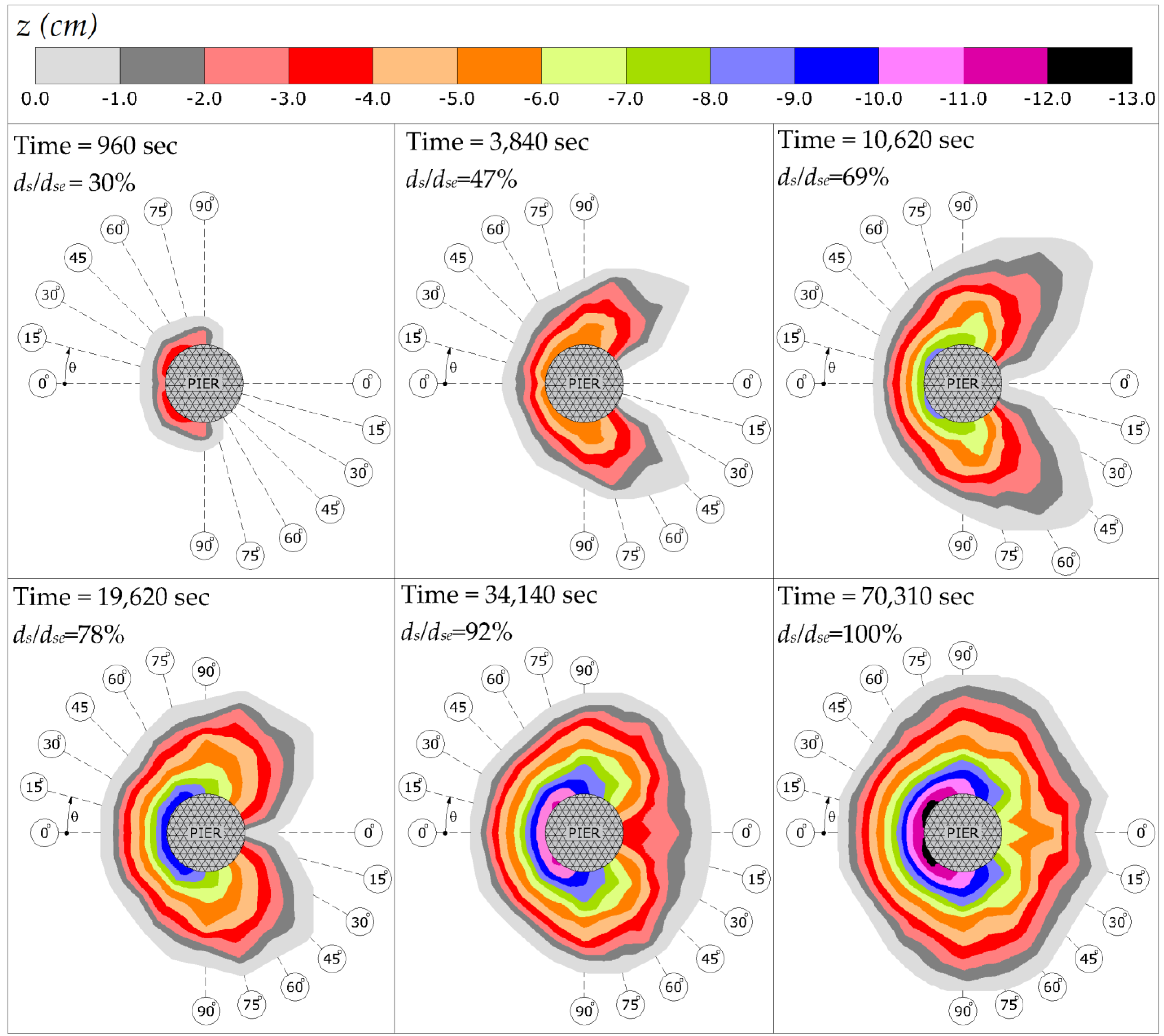
• Tracking the flow structure and bed shear stress variations during the development of a scour hole with the maximum achievable number of development stages. The morphological dimensions for the development stages (seven stages) of the scour hole were collected from previous studies.

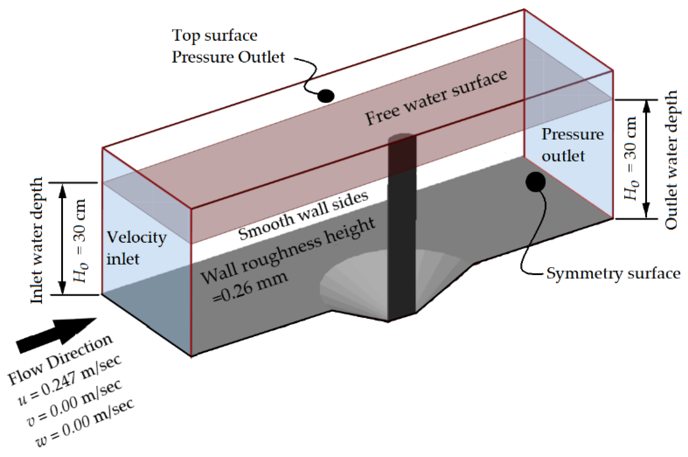
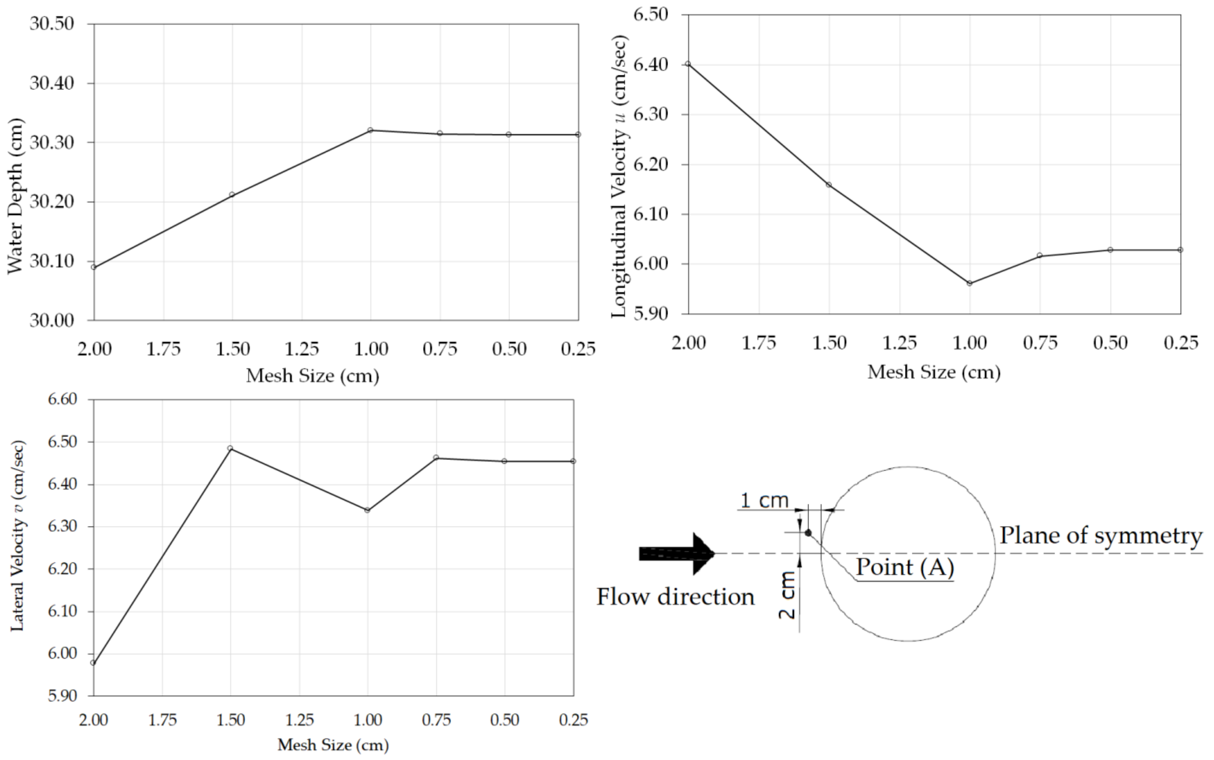
2. Materials and Methods

A three-dimensional CFD with a non-adaptive grid that remained fixed during the calculation process was used to simulate the case in hand. The grid consisted of orthogonal rectangular elements and volumetric hexahedral elements, which eases the mesh generation, enhances the calculation accuracy, and reduces the required memory resources. Flow domain boundaries were defined by calculating the obstacle occupied percentage in the grid elements by applying the Fractional Area Volume Obstacle Representation technique (FAVOR) [44]. The flow continuity (1) and momentum Equations (2)–(4) were modified to comply with the FAVOR technique.

$$\frac{\partial \rho }{\partial t}+\frac{1}{V_F}\rho \nabla \left(\overrightarrow{q}\right)=0$$

(1)

$$\frac{\partial u}{\partial t}+\frac{1}{V_F} \left(\overrightarrow{q}\nabla u\right)=-\frac{1}{\rho }\frac{\partial P}{\partial x}+G_x+f_x$$

(2)

$$\frac{\partial v}{\partial t}+\frac{1}{V_F}\left(\overrightarrow{q}\nabla v\right)=-\frac{1}{\rho }\frac{\partial P}{\partial y}+G_y+f_y$$

(3)

$$\frac{\partial w}{\partial t}+\frac{1}{V_F} \left(\overrightarrow{q}\nabla w\right)=-\frac{1}{\rho }\frac{\partial P}{\partial z}+G_z+f_z$$

(4)

where (V_F) is the opened fraction volume to flow, (x,y,z) are the rectangular cartesian coordinates, $\overrightarrow{A}$ is the area fraction vector (A_x,A_y,A_z) opened to flow, $\overrightarrow{V}$ is the velocity vector and its flow components, (u,v,w) are the instantaneous velocity components in rectangular Cartesian coordinates, $\left(\overrightarrow{q}\right)$ is the flux vector and its components (u.A_x,v.A_y,w.A_z), (ρ) is the fluid density, (G_x,G_y,G_z) are the water body acceleration in (x,y,z) directions,(f_x,f_y,f_z) are the viscous accelerations in (x,y,z) directions, (t) is the time, and (P) is the pressure.

The Volume of Fluid algorithm (VOF) developed by the authors of [45] was used to capture the fluid free surface. The function (F) represents the percentage of fluid occupancy percentage for each grid cell, with values that range between 0 and 100%. The perpendicular line to the rapid change direction of the (F) value represents the free surface inside the grid cell as shown in Figure 1.

$$\frac{\partial F}{\partial t}+\frac{1}{V_F}F \nabla \left(\overrightarrow{q}\right)=0$$

(5)

The available CFD techniques have a limited ability in simulating the scour and erosion processes, thus limiting their trusted applicability in scour depth estimation [43]. In the present study, to investigate the flow structure during the scouring process, the flow conditions and the bathymetry changes of the scour hole during the development of the scouring process were obtained from the experimental work found in [46]. The experimental work was conducted at the Darmstadt University of Technology, the Institute of Hydraulic and Water Resources Engineering, Germany. The scour development around a 20 cm diameter (D), sand-embedded Plexiglas pier was investigated at different time steps (960, 3840, 10,620, 19,620, 34,140, and 70,320 s). The bathymetry of the scour hole at each time step was measured using a Laser Distance Sensor (LDS) with $\pm 4\mathrm{mm}$ accuracy located at the pier center and vertically driven with $\pm 0.02\mathrm{mm}$ precision. Sand of D₅₀ = 0.6 mm, with the standard deviation of particle size (σ_g = 1.37), and an angle of repose = 30° was used to form a 50 cm depth movable bed material in the working section of a glass-sided rectangular flume that was 26.0 m long with a 2.0 m width, and a 1.0 m depth. The working section was located at $16.0\mathrm{m}$ downstream from the flume entrance with the same width as the flume and was extended for $4.0\mathrm{m}$. The flume tailgate was used to maintain a $30.0\mathrm{cm}$ water depth (H_o) above the original bed level and a $0.247\mathrm{m}/\mathrm{s}$ average cross-section velocity. The average cross-section velocity was selected to provide $95\%$ of the critical bed shear stress. The experiments lasted for 21 h to achieve equilibrium conditions where the variation in the scour depth does not exceed D₅₀ in one hour. Figure 2 shows the contour lines of the developed scour hole at different time steps with the maximum scour depth (d_S) at the concerned time step, until the equilibrium conditions with maximum scour depth (d_Se) were reached which were selected as the geometric files for the current study. Auto-CAD software was utilized to generate a Stereolithographic (STL) file for each scour hole geometry in addition to the flat-bed conditions, by approximating the solid surfaces with triangles. Figure 3 illustrates the Cartesian coordinate system used in the description of the results obtained from the CFD simulations. The full-scale geometry model was constructed with the boundary conditions shown in Figure 4.

The Courant number is one of the key factors which should be considered for a proper numerical simulation since it represents the ratio between the distance traveled by the flow and the grid cell length in the direction of flow through a single numerical simulation time step. In the current study, the Courant number stability criterion equaling to unity was achieved by applying an adjustable variable time step (δ_t) since the grid size was uniform along with the calculation domain.

$${\delta }_t<min\left(\frac{V_F{\delta }_{x_i}}{A_{x}u},\frac{V_F{\delta }_{Y_j}}{A_{y}v},\frac{V_F{\delta }_{z_k}}{A_{z}w}\right)$$

(6)

where (δx_i, δy_j, δz_k) are the cell sizes in the rectangular Cartesian coordinates.

Mesh sensitivity analysis is one of the mandatory CFD steps that enables an acceptable accuracy in the results to be reached with the efficient usage of computational resources. The variation of water depth, lateral velocity, and longitudinal velocity with different grid sizes starting from $2.00\mathrm{cm}$ to $0.25\mathrm{cm}$ were evaluated. These hydraulic parameters were calculated at point A, which was selected at $1.0\mathrm{cm}$ upstream of the pier and $2.0\mathrm{cm}$ away from the symmetry plane as shown in Figure 5. The calculated values of the hydraulic parameters remained almost constant for the mesh sizes $0.50$ and $0.25\mathrm{cm}$. Accordingly, a 0.5 cm grid size was selected to generate the mesh for the current study. The selected grid size satisfied the wall function limitations (30 < Z⁺ < 100) to avoid calculations in the viscous sublayer and to ensure that the law of the wall was applicable.

Table 1. Variation of the domain cell numbers for the current study simulations.

Run Number	Total Domain Cells	Fluid Sub Domain Cells	Solid Sub Domain Cells	Partially Wet Cells
1-(ds/dse = 0.00%)	13,764,080	8,870,812	179,306	4,713,962
2-(ds/dse = 30.0%)	13,764,080	8,874,962	180,935	4,708,183
3-(ds/dse = 47.0%)	13,764,080	8,888,140	184,195	4,691,745
4-(ds/dse = 69.0%)	13,764,080	8,903,531	187,177	4,673,372
5-(ds/dse = 78.0%)	13,764,080	8,910,260	187,515	4,666,305
6-(ds/dse = 92.0%)	13,764,080	8,922,547	188,995	4,652,538
7-(ds/dse = 100.0%)	13,764,080	8,940,817	191,613	4,631,650

shows the variation in the CFD model cell types and numbers while using the selected $0.5\mathrm{cm}$ grid size in the three Cartesian directions for the seven scour hole stages starting from $ds/dse=0.00\%$ to $ds/dse=100.0\%$.

$$Z^{+}=\frac{u_{*}z}{\upsilon }$$

(7)

where (Z⁺) is a dimensionless parameter for the wall function, (U_*) is the shear velocity, (z) is the distance from the cell centroid to the wall, and (υ) is the kinematic viscosity.

The turbulence phenomenon is characterized by its spatial and temporal rapid changes in the flow field. To capture the turbulence by applying mass and momentum conservation equations, the use of a very small grid resolution with a very small-time step is required. The available computational and storage resources have not been sufficient until now to conduct such a fine-scale simulation [44]. Turbulence simplified models can simulate the turbulence effect on flow parameters. Recently, LES turbulence modeling has gained increasing attention, and was used for the first time to investigate the flow field and the scouring potential around piers in 2013 [47]. The LES requires vast computational and storage resources, which are not readily available for personal computer-based CFD simulations. The Reynolds Averaged Navier Stokes (RANS) turbulence models provide an inexpensive solution for the CFD simulation of the turbulence effect on flow parameters. No agreement among the researchers has been achieved in the literature for the most suitable turbulence model to be used in similar cases to the current study. The Renormalization Group RNG k-ε turbulence model was recommended by the authors of [32], the k-ε turbulence model was recommended by the authors of [27,28,29], and the k-ω turbulence model was recommended by the authors of [30,31]. The three turbulence models RNG k-ε, k-ε, and k-ω are evaluated in the current study. All turbulence models reached steady-state conditions upstream from the pier at relatively small simulation times. At the downstream side, a longer simulation time for the k-ε and RNG k-ε turbulence models was required, and no steady-state conditions were achieved for the k-ω turbulence model. The numerical model simulated velocities u and v in their normalized form and $u$/U_o and v/U_o were validated against the experimental measurements obtained from [30] as shown in Figure 6 and Figure 7.

The results obtained from the three turbulence models were almost identical at the upstream side of the pier. At the pier’s downstream side, the k-ε and RNG k-ε turbulence models reached steady state conditions, which is not the case in reality due to the existence of vortices and oscillations at the downstream side. The k-ω turbulence model did not reach steady state conditions at the pier’s downstream side and considerable flow oscillations were obtained. Figure 8 shows the resulting longitudinal velocity oscillation at the pier’s downstream side for 10 s with a 0.5 s interval. The average values of the velocities in both the longitudinal and vertical directions show a non-uniform pattern close to the measured values near the pier as in the experimental results given in Figure 6 and Figure 7.

The tested turbulence models’ base line is two transport equations for the turbulence kinetic energy (k) and the turbulence dissipation (ε or ω). The k-ε model is very powerful in the simulation of different flow conditions but the lack of sensitivity to adverse pressure gradients is one of the well-known shortcomings. The k-ε model predicted significantly higher shear stresses which delay or completely prevent separation. On the other hand, the k-ω model had a better performance in relation to the adverse pressure gradient [48] which led to the achieved velocity fluctuations.

It can be concluded that the k-ω turbulence model is capable of capturing the flow oscillations and vortex shedding at the downstream side of the pier. The k-ω turbulence model results are more accurate than the k-ε and RNG k-ε turbulence models and are achievable with affordable computational resources compared to the required resourced for the LES and DES turbulence models.

Accordingly, the k-ω turbulence model was selected to simulate the turbulence effect on the flow pattern in the current study.

In all the seven CFD simulations that were performed (d_S/d_Se = 0, 30, 47, 69, 78, 92, and 100%) the following model parameters were assigned; ($0.5\mathrm{cm}$ grid size in the three Cartesian directions, depth-averaged approach velocity U_o = 0.247 m/s at the velocity inlet boundary, water depth H_o = 30 cm at the domain’s upstream and downstream sides, and the k-ω turbulence model). The flow velocities, vorticities, and bed shear stress were obtained from each simulation.

3. Results and Discussion

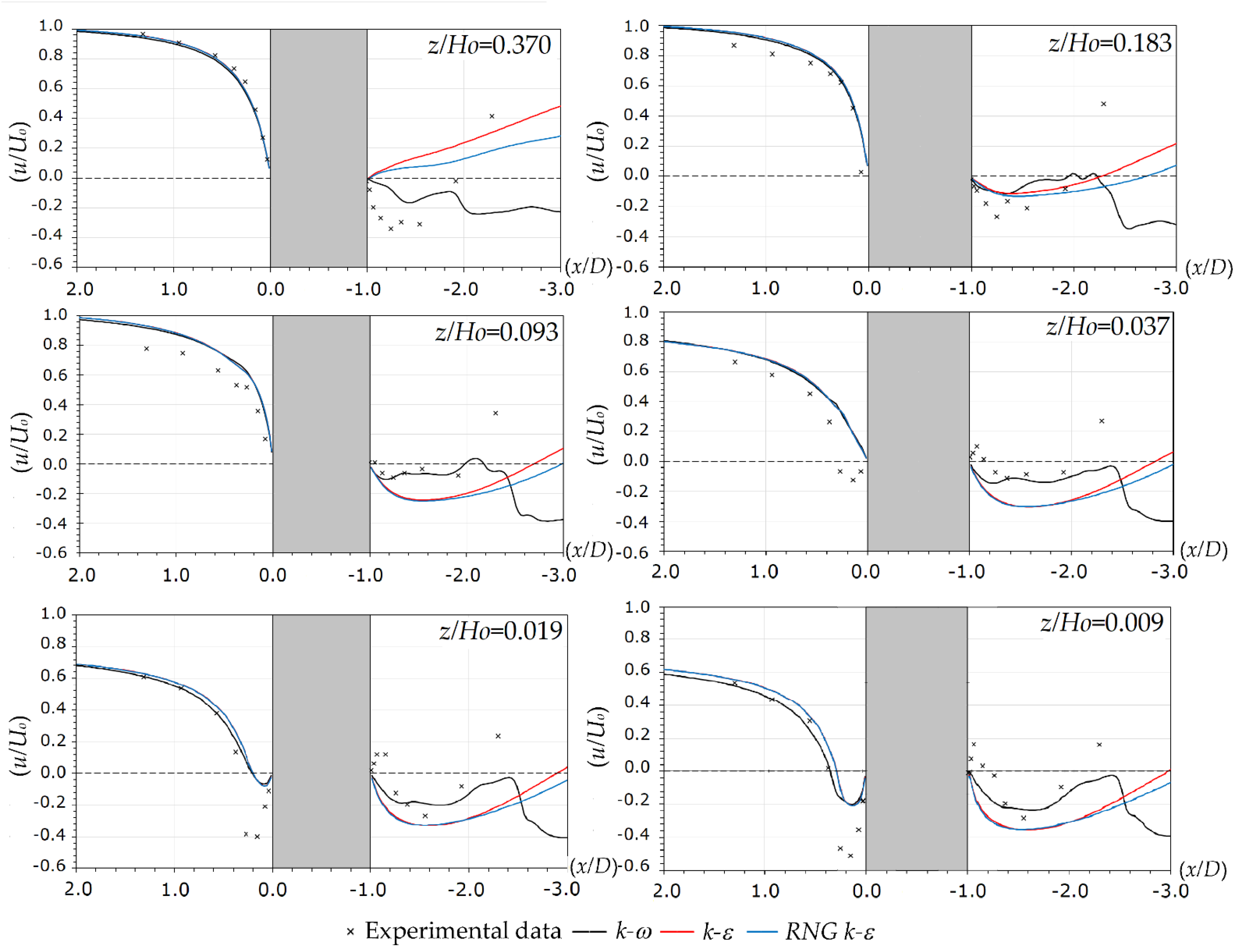
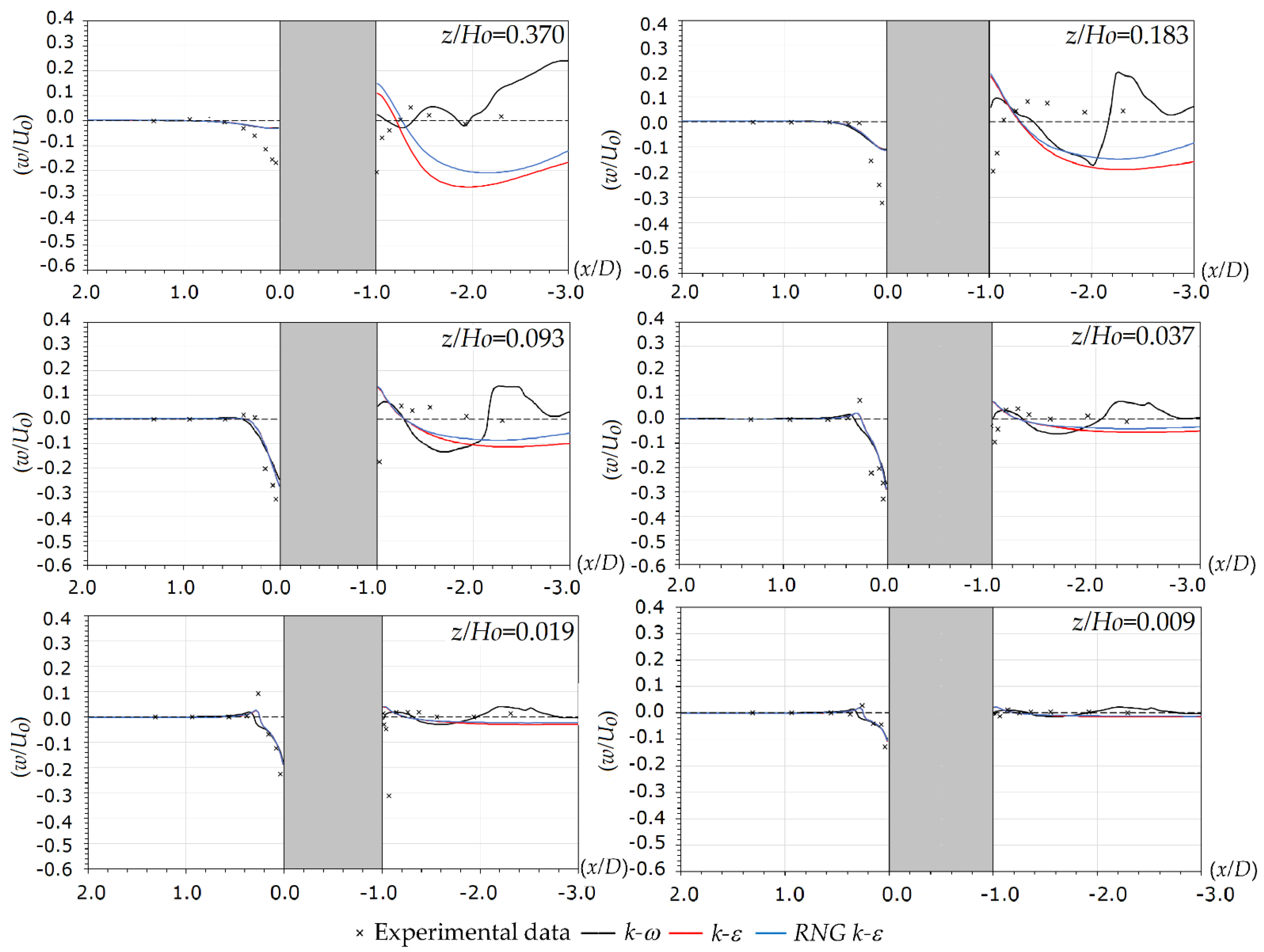
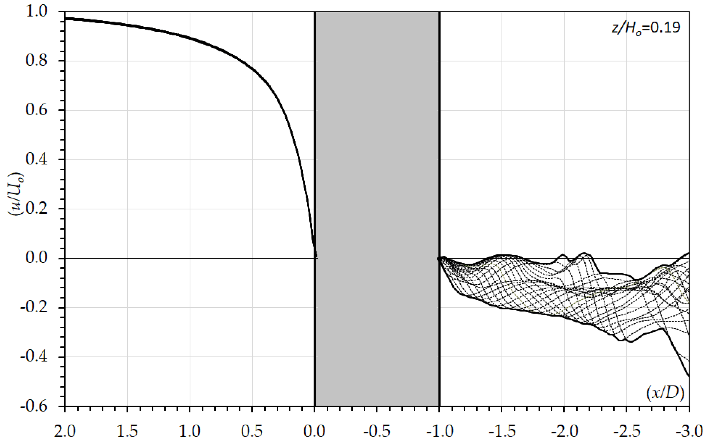
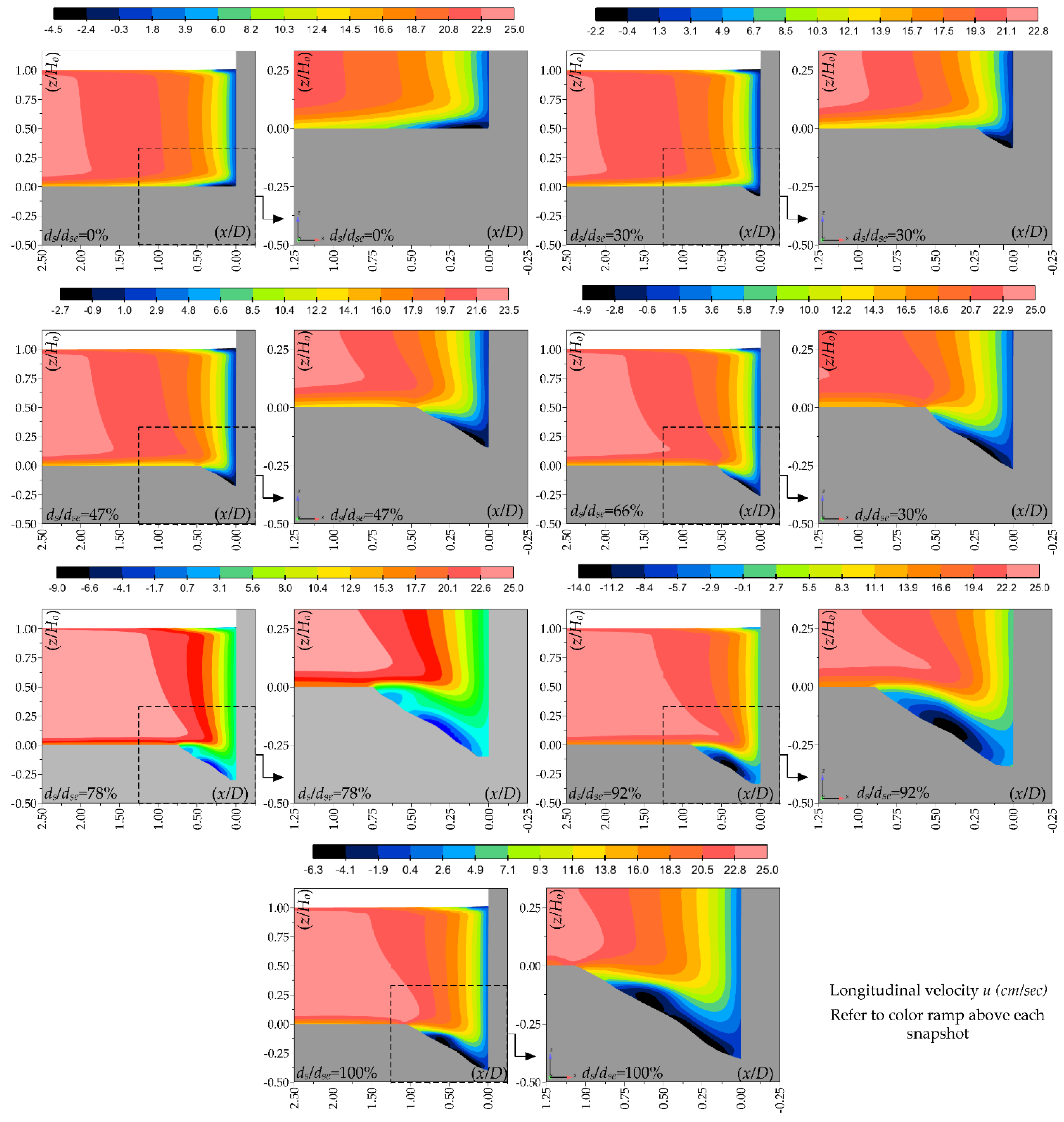
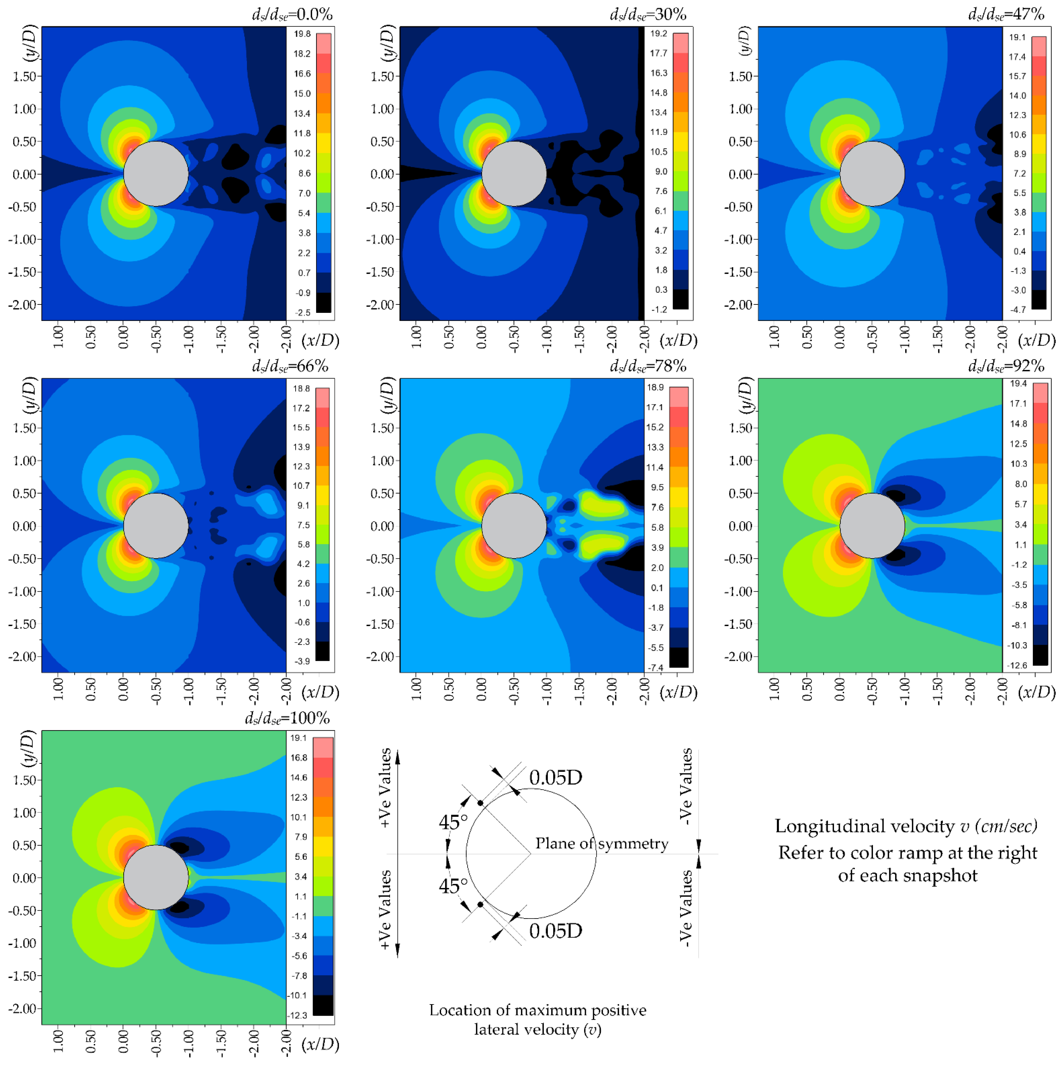
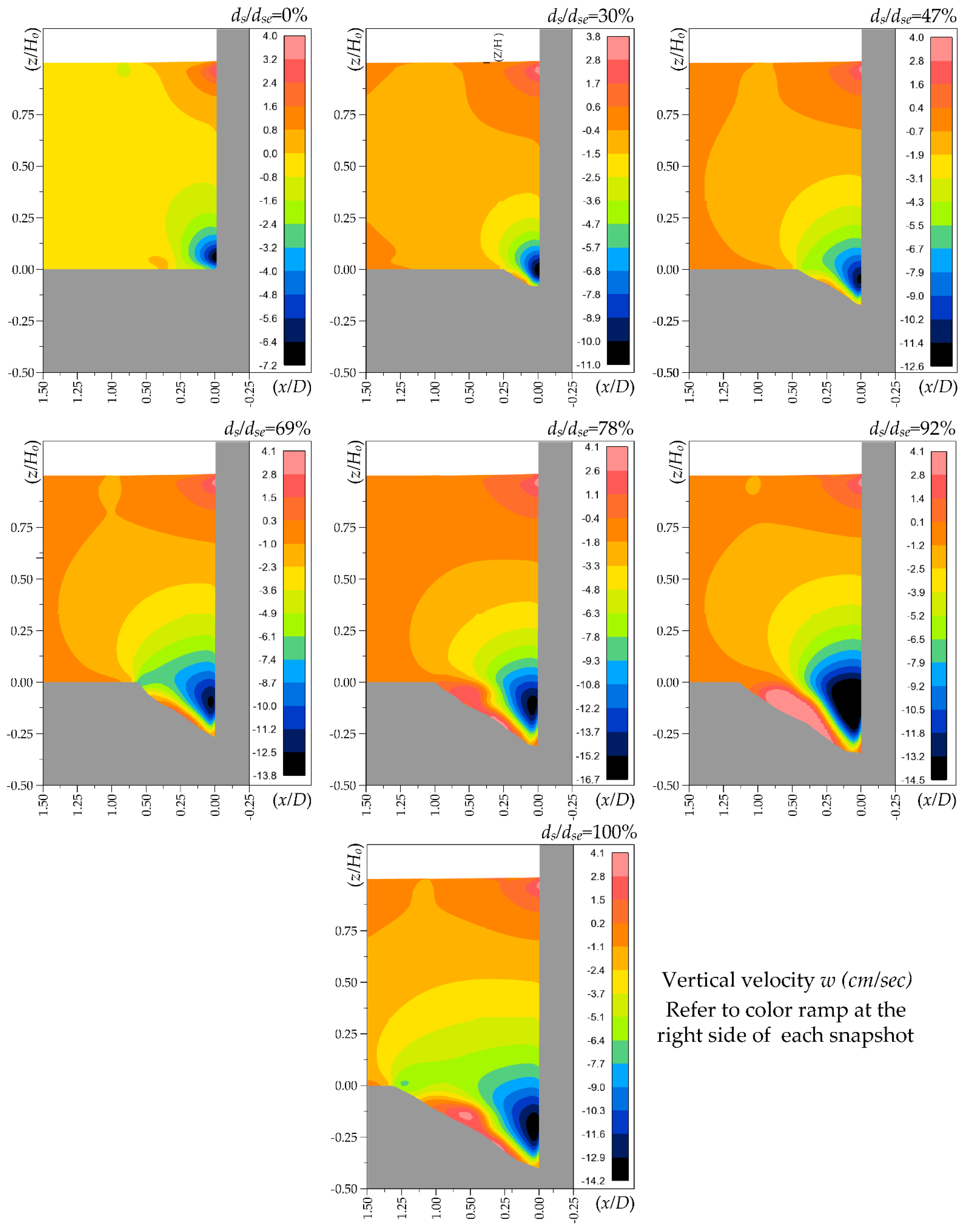
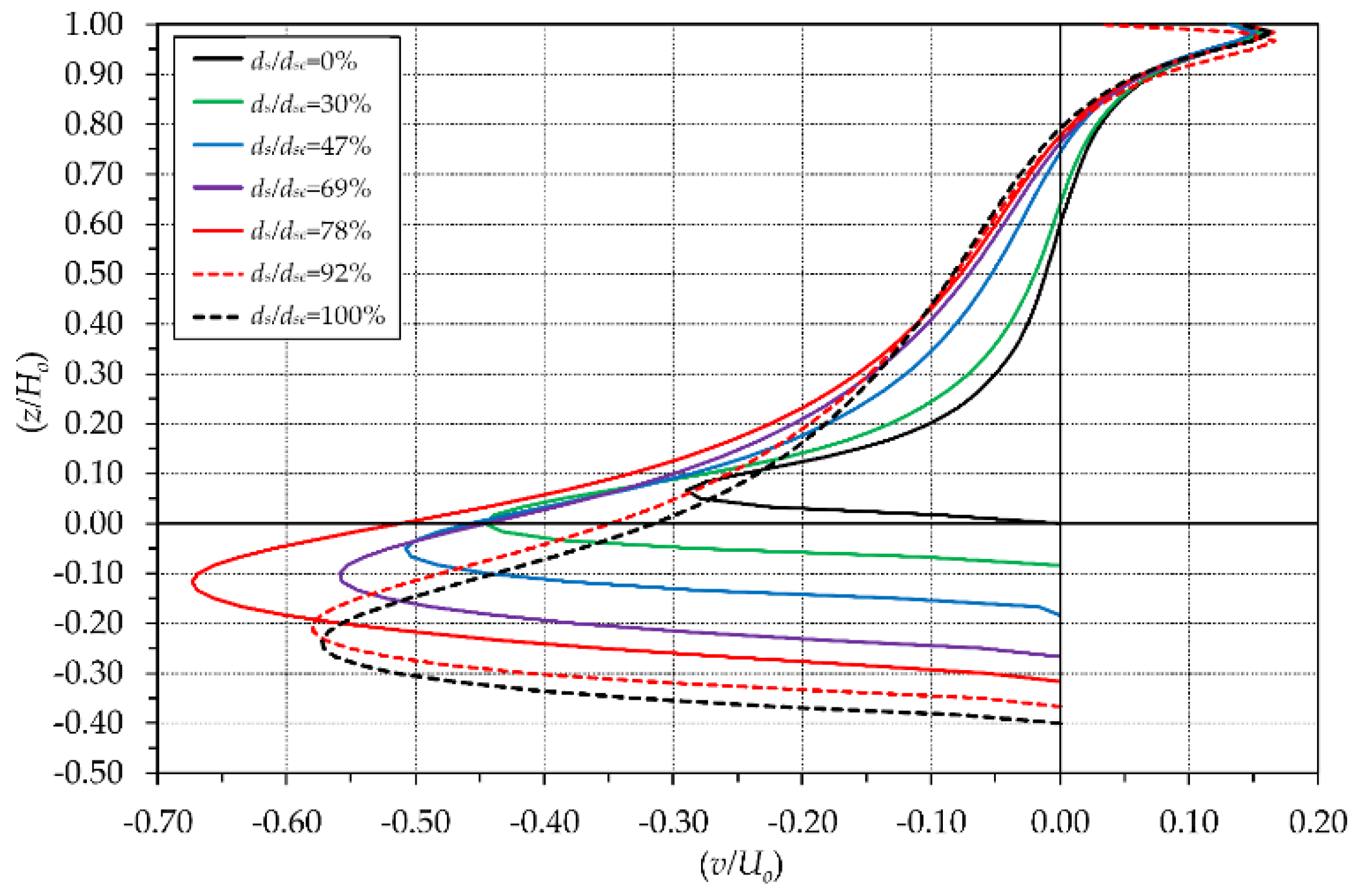
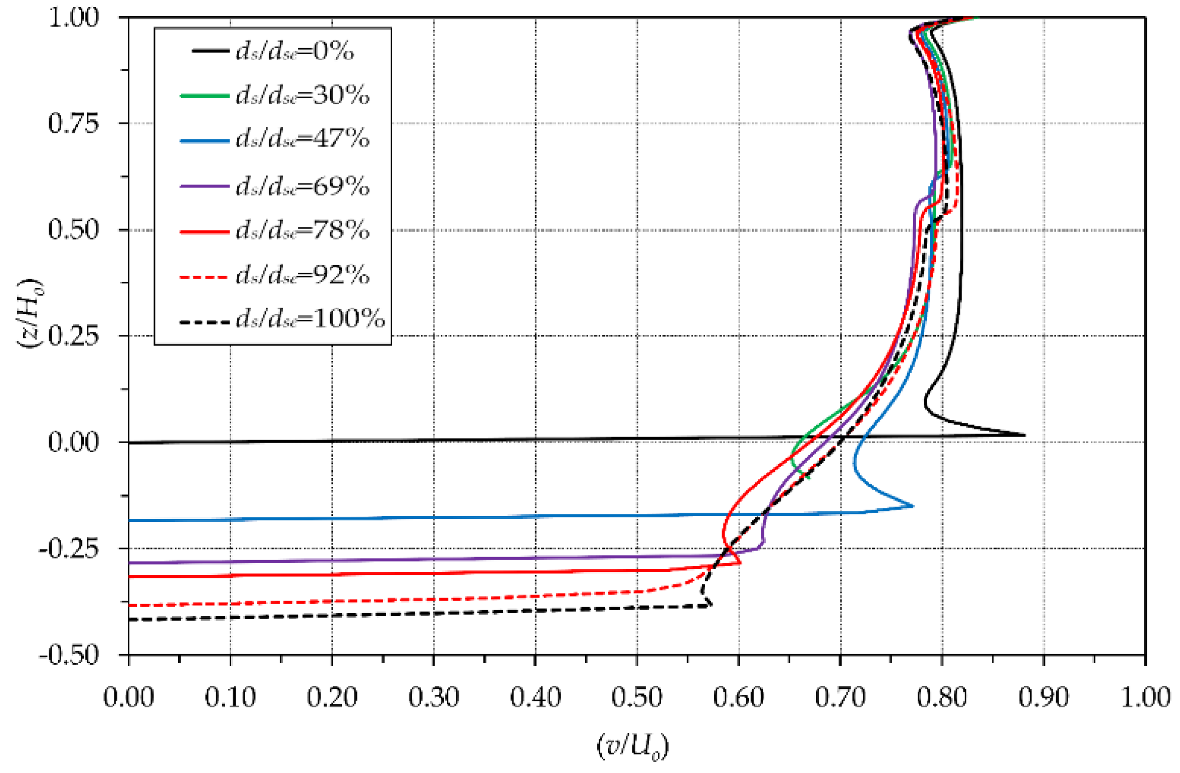
3.1. Velocity Field Description

The longitudinal velocity U decreased at the vertical plane of symmetry as the flow approached the pier before reaching stagnation at the pier’s upstream face. The decrease became noticeable approximately at x/D = 2.0, as shown in Figure 9. A zone of reversal flow was noticed at x/D = 0.2 upstream from the pier at flat-bed conditions, then it moved further upstream from the pier towards the scour hole edge, and downward towards the scour hole bed in conjunction with the progress of the scour hole. These observations indicate that as the scour hole developed, the HV sunk inside the hole and moved further below the original bed level, which is in agreement with the experimental observations by the author of [14]. The reversal longitudinal flow reached a maximum value of −0.55U_o at d_S/d_Se = 0.92 and reduced to −0.25U_o at the equilibrium scour stage.

The transversal velocity v appeared at x = 2D indicating the transformation from a two-dimensional to a three-dimensional flow. The maximum positive lateral velocity was located at a radial distance = 0.05D measured from the pier surface and formed 45° on the two sides of the plane of symmetry upstream from the pier, as shown in the lateral velocity distribution at Z/H_o = 0.5 in Figure 10. The maximum positive values of the lateral velocity remained almost constant in the order of about 0.8U_o during the souring process and reached (0.0) at the bottom level, as shown in the vertical profiles given in Figure 11.

Figure 12 shows the vertical velocity w distribution in the plane of symmetry upstream of the pier, through the development of the scouring process. As the flow approached the pier, the vertical velocity components remained approximately negligible until X/D = 1.0 then started to appear and subsequently grow considerably in the downstream direction towards the pier. The maximum downward vertical velocity occurred at a distance range of 0.02D:0.05D which is in agreement with the laboratory observations in [12]. Figure 13 shows the variation of the vertical velocity profiles in the plane of symmetry during the scouring process at a distance of 0.05D upstream of the pier. The downward vertical velocity increased with the progress of the scour hole until reaching its maximum value of −0.67U_o at d_S/d_Se = 0.78. This value lies between the −0.6U_o stated by the authors of [16,17], and the −0.8U_o stated by the author of [14]. The downward velocity decreased with the development of the scour hole from d_S/d_Se = 0.78 to d_S/d_Se = 1.0 until reaching a value of −0.57U_o at d_S/d_Se = 1.00. The increase in the downward velocity until d_S/d_Se = 0.78 then the decrease till d_S/d_Se = 1.00 explains the experimental observation in [46] about the formation of the vertical trench just upstream of the pier at intermediate scour stages and its disappearance in the equilibrium stage. The maximum magnitude of the upward velocity was $0.17U_o$ at Z/H_o = 0.95 during all stages. The upward flow near the free surface formed a circulation that is called bow wave, causing the flow depth to increase in front of the pier.

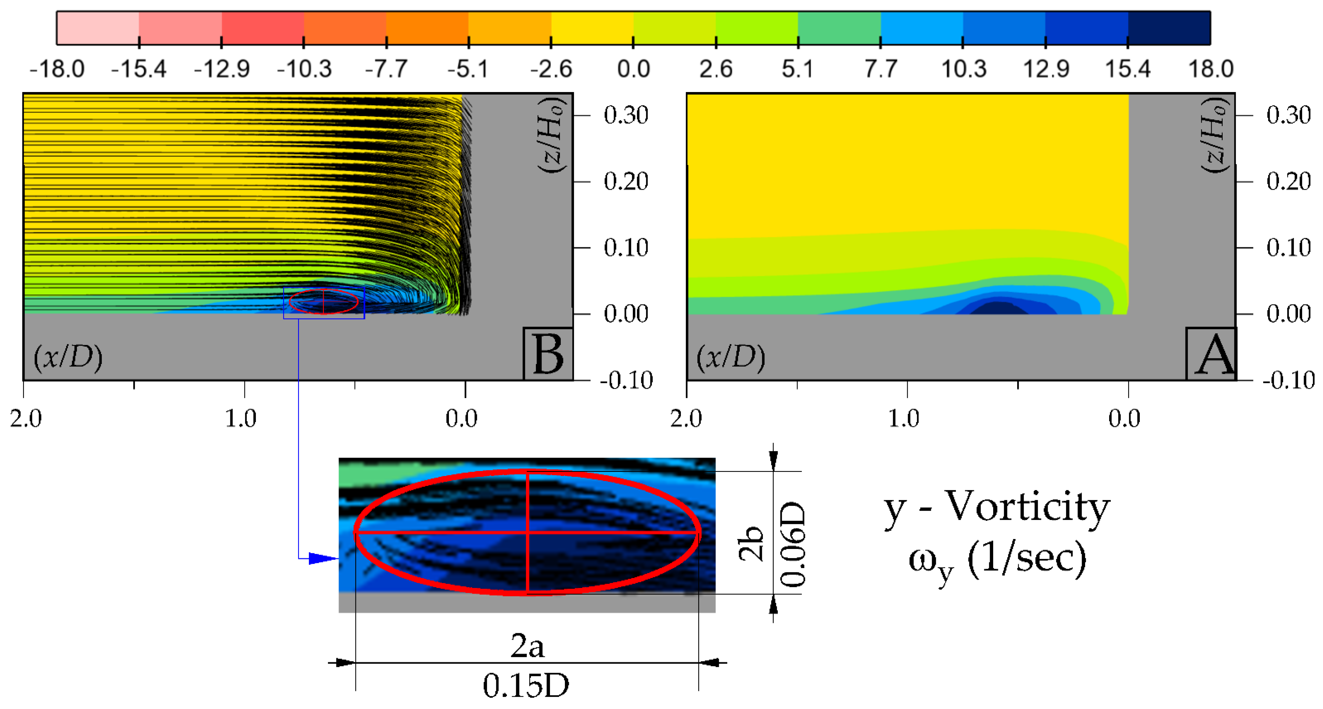
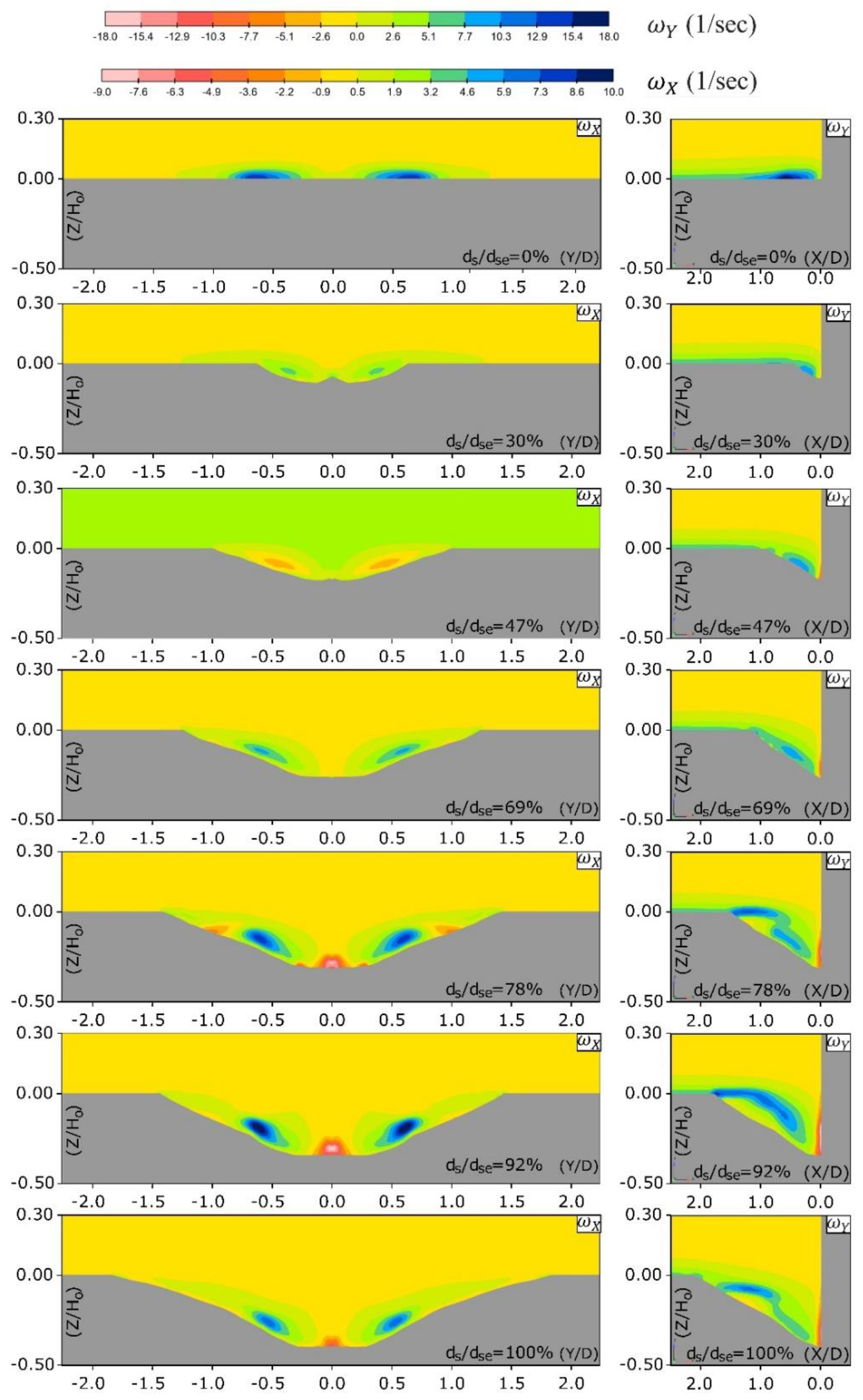
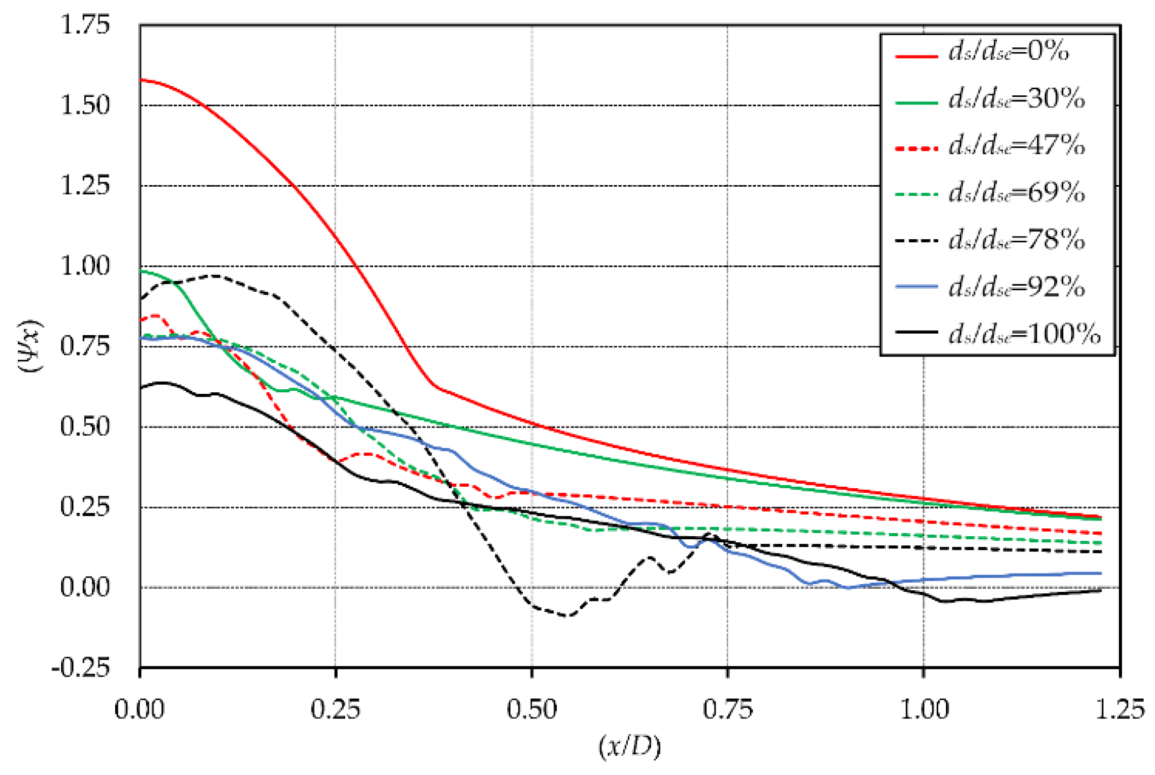
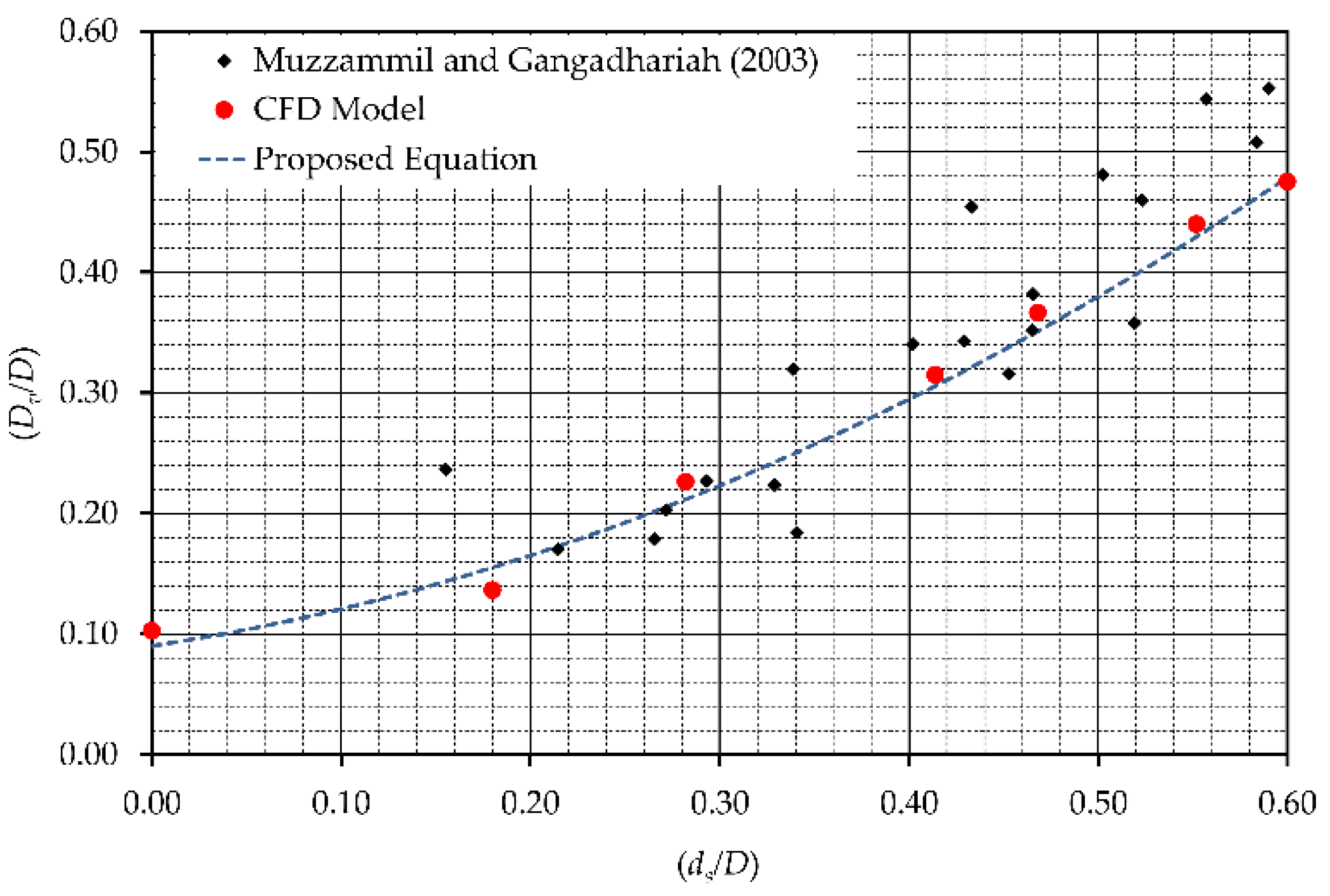
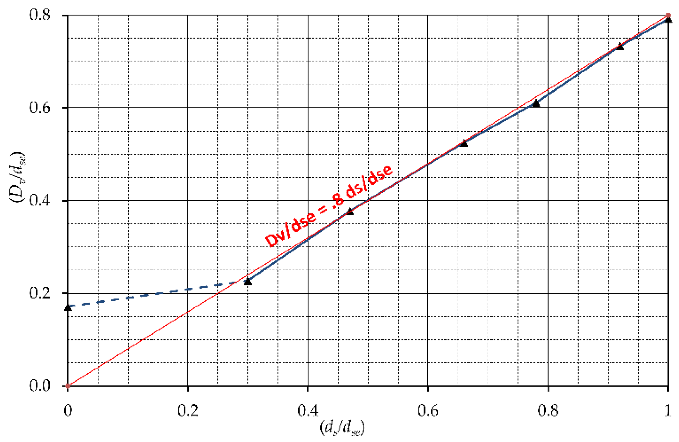
3.2. Horseshoe Vortex

In the current study, dense longitudinal and transversal sections with 0.025D spacing were utilized to investigate the structure and the evolution of the HV characteristics during the scouring process. The development of the scouring process presented in the CFD model geometry by using seven solidified bed bathymetries was captured experimentally during the progress of the scour hole until the equilibrium scour bed was reached. Vorticity, or circulation per unit area, reflects the tendency for fluid elements to spin. It is essential to know the magnitude of circulation as it implies the strength of the vortex. The out of plane vorticity on the longitudinal sections and the transversal sections are $\left({\omega }_Y\right)$, and $\left({\omega }_X\right)$, respectively, and are determined as follows:

$${\omega }_Y=\frac{\partial u}{{\partial }_Z}-\frac{\partial w}{{\partial }_X}$$

(8)

$${\omega }_X=\frac{\partial w}{{\partial }_Y}-\frac{\partial v}{{\partial }_Z}$$

(9)

Figure 14 shows the contours of Y-vorticity (${\omega }_Y$) and shows that the flow streamlined upstream from the pier at the plane of symmetry at flat-bed conditions. The interaction between the downward flow and the horizontal flow close to the original flat-bed surface initiates the formation of a primary rotating clockwise HV vortex. The shape of the vortex in the flat-bed case was almost elliptical in cross-section with a major horizontal axis. The size of the HV vortex is presented by the mean vortex size $D_V=a+b$ as proposed by the authors of [49]. In flat-bed conditions, the height (length of the minor axis) of the elliptical vortex at the plane of symmetry is approximately 40% of the length of the major axis, and the size of the vortex is about $0.1D$. Figure 15 gives the contour lines of y-vorticity $\left({\omega }_Y\right)$, and x-vorticity $\left({\omega }_X\right)$ during the progress of the scour hole starting from the flat-bed until the equilibrium conditions were reached. It is clear from Figure 15 that as the scour hole developed, the HV vortex sunk into the scour hole and was kept contained within its boundaries.

Circulation or vortex strength $\left(\Gamma \right)$ at any surface was computed using the out of plane vorticity contours, $\left({\omega }_i\right)$ and applying the Stokes theorem as follows:

$$\Gamma ={{\displaystyle \oint }}_c^{}\overline{V} d_{dis}={{\displaystyle \iint }}_A^{}{\omega }_i dA$$

(10)

where $\overline{V}$ is the velocity vector, $d_{dis}$ is the differential displacement vector along with a closed curve C, and A is the enclosed area. The area-averaged dimensionless circulation $({\Psi }_i)$ was developed to eliminate the area effect in the assessment of the development of the vortex strength. The selected enclosed area for the vortex strength calculation upstream of the pier was chosen to ensure the containment of the HV vortex during all stages of the scouring process in longitudinal and transversal directions.

$${\Psi }_i={\Gamma }_i D/\left(U_o A\right)$$

(11)

It is clear from Figure 16 and Figure 17 that the circulation in the $y$ direction was the main driving factor in the development of the scouring process, since it reached about 4 to 5 times the circulation in the $x$ direction. The area-averaged dimensionless circulation in both the $x$ and $y$ directions decreased with the development of the scour hole, starting from its maximum values at the flat-bed condition.

${\Psi }_{Y-\mathrm{flatbed}}$ reached its maximum value at the pier centerline where $y/D=0$ and decreased laterally until reaching a constant value of $0.7\times {\Psi }_{y-flatbed-maximum}$ at $y/D=1.2$. As the scour developed and the scour hole started to increase, this trend of lateral variation of ${\Psi }_y$ was reversed starting from $d_s/d_{se}=0.47$to have its minimum value near the pier centerline and increased until reaching the same constant value of the value of $0.7\times {\Psi }_{y-flatbed-maimum}$ at the edge of the scour hole.

The development of the mean size of the HV vortex during the development of the scour hole is in good agreement with the experimental data obtained from [49], as shown in Figure 18. Based on the present study results, a theoretical relationship is developed for calculating the relative mean vortex size $D_V/D$ as a function of the relative scour depth $d_s/D$ as follows:

$$D_V/D=0.67{\left(d_s/D\right)}^2+0.24\left(d_s/D\right)+0.1$$

(12)

The ratio between the HV vortex mean size and the scoring depth $D_v/d_s$ remained constant with a value of $0.8$ during the development of the scour hole starting from $d_s/d_{se}=0.3$ until the equilibrium scouring stage was reached, as shown in Figure 19. The 0.8 ratio is considered as a simplification for Equation (12) and valid for $d_s/d_{se}\ge 0.3$.

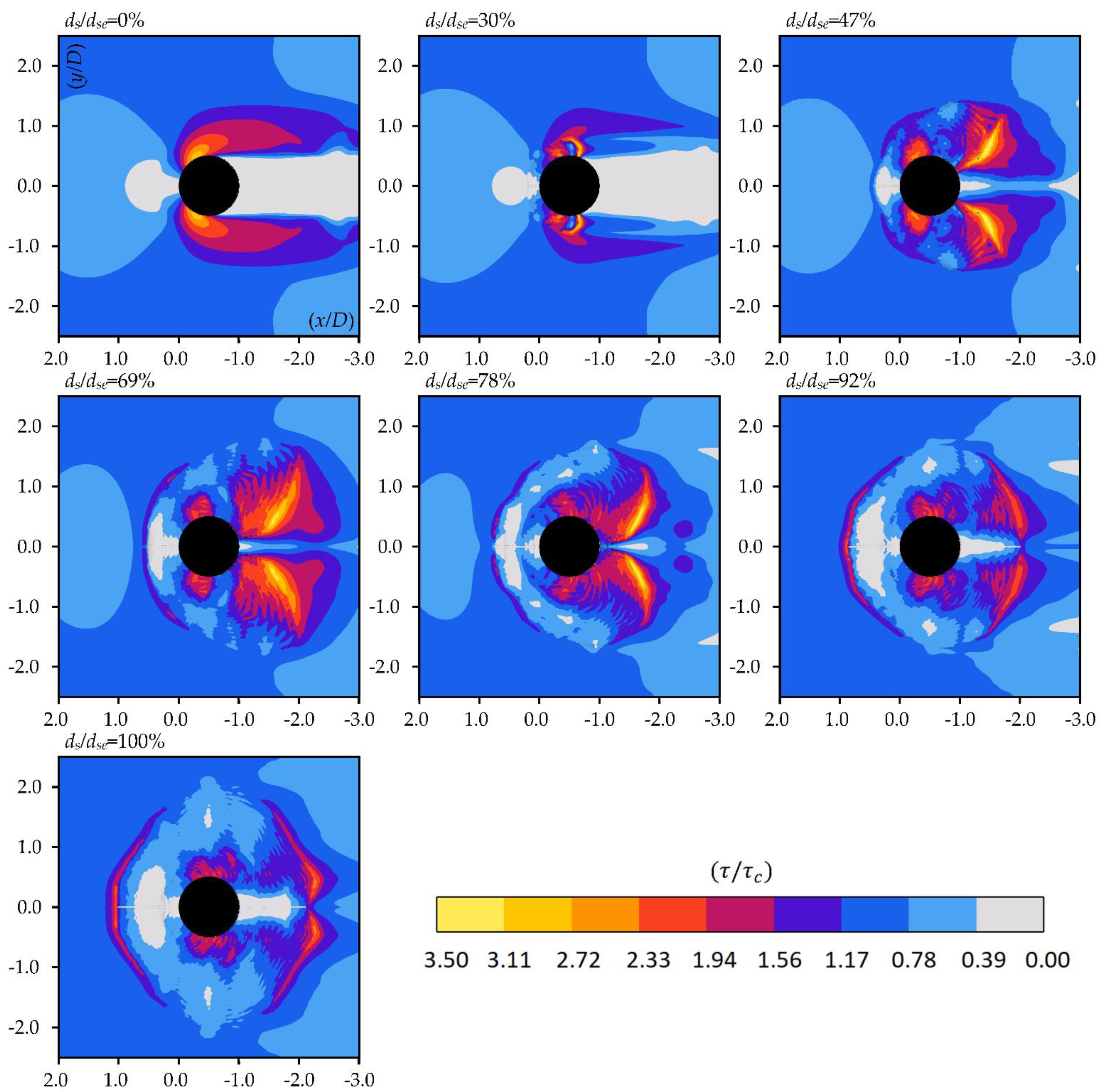
3.3. Bed Shear Stress

The variation of the bed shear stress distribution was monitored through the scour stages. The critical bed shear stress for the experiment used specific grain sizes $({\tau }_c=0.2\mathrm{N}/{\mathrm{m}}^2$) [50]. The maximum value of the bed shear stress at the equilibrium scour hole $({\tau }_{e-maximum}$) reached $0.45\mathrm{N}/{\mathrm{m}}^2$ at two spots located at the downstream edge of the scour hole $\left(\pm {13}^{°}\right)$ which was an overestimation. The overestimation is reported in many CFD simulations with different turbulence models as reported by the authors of [32,51]. Figure 20 shows the variation of the normalized bed shear stress $(\tau /{\tau }_{e-maximum})$.

The location of the maximum bed shear stress in flat-bed conditions was located where the scour starts $\left(\pm {100}^{°}\right)$ with $\tau /{\tau }_c=3.3$. With the development of the scour hole, the high values of bed shear stress became confined within the scour hole, and the maximum values were located at the scour hole’s downstream edges within the range $\left(\pm {13}^{°}\right)$ to $\left(\pm {40}^{°}\right)$ for ds/dse > 30%, and at the location where scour started $\left(\pm {100}^{°}\right)$. The distribution of the bed shear stress was logical and matched the progress of the scour hole.

4. Conclusions

A three dimensional CFD model was used to simulate the flow pattern around circular bridge piers during the development of the scour hole with a uniform mesh size of 0.025D. Seven geometries of the scour hole were captured experimentally during the development of the scouring process [46]. The seven geometries were utilized to prepare the geometric file for each CFD simulation to represent scour development. The simulated scour stages were 0.0%, 30%, 47%, 69%,78%, 92%, and 100% of the equilibrium scour hole. The numerical results were verified against the experimental findings of the authors of [12,14,30,49].

Three turbulence models were evaluated in the current study. The $k-\omega$ turbulence model captured the flow oscillations at the downstream side of the pier with economical computational resources. The $k-\omega$ turbulence model was selected to simulate the turbulence in the CFD numerical simulations for the current study due to its proven accuracy in capturing flow oscillations at the downstream side of the pier with relatively economical computational resources.

A detailed description of the flow field was introduced, and it was concluded that:

• The reversal longitudinal flow reached a maximum value of $-0.55U_o$ at $d_s/d_{se}=0.92$ and reduced to $-0.25U_o$ at the equilibrium scour stage;
• The maximum positive values of the lateral velocity remained almost constant in the order of about $0.80U_o$ during the souring process and reached 0.0 at the bottom level;
• The downward vertical velocity increased with the progress of the scour hole until reaching its maximum value of $-0.67U_o$ at $d_s/d_{se}=0.78$;
• As the scour hole developed, the HV vortex sunk into the scour hole and was kept contained within its boundaries.

The area-averaged dimensionless circulation ${\Psi }_i$ was developed to allow for the assessment of the development of the vortex strength through the scouring process by eliminating the calculation area effect. It was concluded that the circulation in the $Y$ direction was the main driving factor in the development of the scouring process more than the circulation in the $X$ direction.

The relationship between the relative mean vortex size $D_v/D$ and the relative scour depth $d_s/D$ was developed as $D_V/D=0.67{\left(d_s/D\right)}^2+0.24\left(d_s/D\right)+0.1$. As a simplification for the previous equation, the ratio between the HV vortex mean size and the scoring depth $d_v/d_s$ and $d_s/d_{se}$ remained constant with a value of $0.8$ during the development. The 0.8 ratio was valid for $d_s/d_{se}\ge 0.3$ until the equilibrium scouring stage was reached.

The maximum values of bed shear stress were located at the scour hole’s downstream edges within the range $\left(\pm {13}^{°}\right)$ to $\left(\pm {40}^{°}\right)$ and at the location where the scour started $\left(\pm {100}^{°}\right)$. These locations remained steady for $d_s/d_{se}>0.3$ until the equilibrium conditions were reached. The current CFD numerical simulation overestimated the values of bed shear stress. This overestimation is reported in many CFD simulations.

References

1. Laursen, E.M.; Toch, A. Scour around Bridge Piers and Abutments; Bulletin No. 4; Iowa Highway Research Board (IHRB): Iowa, IA, USA, 1956. [Google Scholar]
2. Shen, H.W.; Schneider, V.R.; Karaki, S. Local Scour Around Bridge Piers. J. Hydraul. Div. ASCE 1969, 95, 1919–1940. [Google Scholar] [CrossRef]
3. Breusers, H.N.C.; Nicollet, G.; Shen, H.W. Local Scour Around Cylindrical Piers. J. Hydraul. Res. 1977, 15, 211–252. [Google Scholar] [CrossRef]
4. Jain, S.C.; Fischer, E.E. Scour around Circular Bridge Piers at High Froude Numbers; FHWA Report No. FHWA-RD-79-104; FHWA: Washington, DC, USA, 1979. [Google Scholar]
5. Melville, B.W. Local Scour at Bridge Abutments. J. Hydraul. Eng. 1992, 118, 615–631. [Google Scholar] [CrossRef]
6. Richardson, E.V.; Harrison, L.I.; Richardson, J.R.; Davis, S.R. Evaluating Scour at Bridges; Hydraulic Engineering Circular No. 18 (HEC-18); Federal Highway Administration, U.S. Department of Transportation: Washington, DC, USA, 1993. [Google Scholar]
7. Melville, B.W. Pier and abutment scour: Integrated approach. J. Hydraul. Eng. 1997, 123, 125–136. [Google Scholar] [CrossRef]
8. Sheppard, D.M.; Miller, W.J. Live-bed local pier scour experiments. J. Hydraul. Eng. 2006, 132, 635–642. [Google Scholar] [CrossRef] [Green Version]
9. Yanmaz, A.M.; Altinbilek, H.D. Study of time-dependent local scour around bridge piers. J. Hydraul. Eng. 1991, 117, 1247–1268. [Google Scholar] [CrossRef]
10. Sheppard, D.M.; Huseyin, D.; Melville, B.W. Scour at Wide Piers and Long Skewed Piers; The National Academies Press: Washington, DC, USA, 2011. [Google Scholar]
11. Melville, B.W.; Sutherland, A.J. Design Method for Local Scour at Bridge Piers. J. Hydraul. Eng. 1988, 114, 1210–1226. [Google Scholar] [CrossRef]
12. Raudkivi, B.A.J. Functional Trends of Scour at Bridge Piers. J. Hydraul. Div. 1986, 112, 1–13. [Google Scholar] [CrossRef]
13. Chiew, Y.-M. Scour protection at bridge piers. J. Hydraul. Eng. 1992, 118, 1260–1269. [Google Scholar] [CrossRef]
14. Melville, B.W. Local Scour at Bridge Sites. Ph.D. Thesis, University of Auckland, Auckland, New Zealand, 1975. [Google Scholar]
15. Ahmed, F.; Rajaratnam, N. Flow around bridge piers. J. Hydraul. Eng. 1998, 124, 288–300. [Google Scholar] [CrossRef]
16. Graf, W.H.; Istirato, L. Flow pattern in the scour hole around a cylinder. J. Hydraul. Res. 2002, 40, 13–20. [Google Scholar] [CrossRef]
17. Dey, S.; Raikar, R.V. Characteristics of horseshoe vortex in developing scour holes at piers. J. Hydraul. Eng. 2007, 133, 399–413. [Google Scholar] [CrossRef]
18. Subhasish, D.; Rajib, D.; Mazumdar, A. Circulation characteristics of horseshoe vortex in scour region around circular piers. Water Sci. Eng. 2013, 6, 59–77. [Google Scholar] [CrossRef]
19. Istirato, L. Experiments on Flow around a Cylinder in a Scoured Channel Bed; Engineering Federal Institute of Technology in Lausanne: Lausanne, Switzerland, 2001. [Google Scholar]
20. Dargahi, B. Flow Field and Local Scouring around a Pier; Bulletin No. TRITA-VBI-137; The Royal Institute of Technology: Stockholm, Sweden, 1987. [Google Scholar]
21. Melville, B.W.; Raudkivi, A.J. Flow characteristics in local scour at bridge piers. J. Hydraul. Res. 1977, 15, 373–380. [Google Scholar] [CrossRef]
22. Richardson, J.E.; Panchang, V.G. Three dimensional simulation of scour-inducing flow at bridge piers. J. Hydraul. Eng. 1998, 124, 530–540. [Google Scholar] [CrossRef]
23. Xiang, Q.; Wei, K.; Li, Y.; Zhang, M.; Qin, S. Experimental and Numerical Investigation of Local Scour for Suspended Square Caisson under Steady Flow. KSCE J. Civ. Eng. 2020. [Google Scholar] [CrossRef]
24. Bao, Y.; Wu, Q.; Zhou, D. Computers & Fluids Numerical investigation of flow around an inline square cylinder array with different spacing ratios. Comput. Fluids 2012, 55, 118–131. [Google Scholar] [CrossRef]
25. Akbari, M.H.; Price, S.J. Numerical investigation of flow patterns for staggered cylinder pairs in cross-flow. J. Fluids Struct. 2005, 20, 533–554. [Google Scholar] [CrossRef]
26. Beheshti, A.A.; Ataie-Ashtiani, B.; Dashtpeyma, H. Numerical simulations of turbulent flow around side-by-side circular piles with different spacing ratios. Int. J. River Basin Manag. 2017, 15, 227–238. [Google Scholar] [CrossRef]
27. Bosch, G.; Rodi, W. Simulation of vortex shedding past a square cylinder with different turbulence models. Int. J. Numer. Methods Fluids 1998, 28, 601–616. [Google Scholar] [CrossRef]
28. Zhi-wen, Z.; Zhen-qing, L. CFD prediction of local scour hole around bridge piers. J. Cent. South Univ. 2012, 19, 273–281. [Google Scholar] [CrossRef]
29. Azhari, A.; Saghravani, S.F.; Mohammadnezhad, B.A. 3D Numerical modelling of local scour around the cylindrical bridge piers. In Proceedings of the XVIII International Conference on Water Resources, Barcelona, Spain, 21–24 June 2010. [Google Scholar]
30. Roulund, A.; Sumer, B.M.; Fredsoe, J.; Michelsen, J. Numerical and experimental investigation of flow and scour around a circular pile. J. Fluid Mech. 2005, 534, 351–401. [Google Scholar] [CrossRef]
31. Baykal, C.; Sumer, B.M.; Fuhrman, D.R.; Jacobsen, N.G.; Fredsøe, J. Numerical investigation of flow and scour around a vertical circular cylinder. Philos. Trans. R. Soc. 2015. [Google Scholar] [CrossRef] [Green Version]
32. Salaheldin, T.M.; Imran, J.; Chaudhry, M.H. Numerical Modeling of Three-Dimensional Flow Field Around Circular Piers. J. Hydraul. Eng. 2004, 130, 91–100. [Google Scholar] [CrossRef]
33. Ali, K.H.M.; Karim, O. Simulation of flow around piers. J. Hydraul. Res. 2002, 40, 161–174. [Google Scholar] [CrossRef]
34. Gopalan, H.; Jaiman, R. Journal of Wind Engineering Numerical study of the flow interference between tandem cylinders employing non-linear hybrid URANS—LES methods. J. Wind Eng. Ind. Aerodyn. 2015, 142, 111–129. [Google Scholar] [CrossRef]
35. Palau-Salvador, G.; Stoesser, T.; Rodi, W. LES of the flow around two cylinders in tandem. J. Fluids Struct. 2008, 24, 1304–1312. [Google Scholar] [CrossRef] [Green Version]
36. Kirkil, G.; Constantinescu, S.G.; Ettema, R. Coherent Structures in the Flow Field around a Circular Cylinder with Scour Hole. J. Hydraul. Eng. 2008, 134, 572–587. [Google Scholar] [CrossRef]
37. Kirkil, G.; Constantinescu, G.; Ettema, R. Detached Eddy Simulation Investigation of Turbulence at a Circular Pier with Scour Hole. J. Hydraul. Eng. 2009, 135, 888–901. [Google Scholar] [CrossRef]
38. Kirkil, G.; Constantinescu, G. Nature of flow and turbulence structure around an in-stream vertical plate in a shallow channel and the implications for sediment erosion. J. Water Resour. Res. 2009, 45, 1–18. [Google Scholar] [CrossRef]
39. Kirkil, G.; Constantinescu, G. Effects of cylinder Reynolds number on the turbulent horseshoe vortex system and near wake of a surface-mounted circular cylinder. Phys. Fluids 2015, 27. [Google Scholar] [CrossRef] [Green Version]
40. Wang, D.; Shao, S.; Li, S.; Shi, Y.; Arikawa, T.; Zhang, H. 3D ISPH erosion model for flow passing a vertical cylinder. J. Fluids Struct. 2018, 78, 374–399. [Google Scholar] [CrossRef]
41. Kazemi, E.; Tait, S.; Shao, S. SPH-based numerical treatment of the interfacial interaction of flow with porous media. Int. J. Numer. Methods Fluids 2020, 92, 219–245. [Google Scholar] [CrossRef]
42. Kazemi, E.; Koll, K.; Tait, S.; Shao, S. SPH modelling of turbulent open channel flow over and within natural gravel beds with rough interfacial boundaries. Adv. Water Resour. 2020, 140, 103557. [Google Scholar] [CrossRef]
43. Ettema, R.; Constantinescu, G.; Melville, B.W. Flow-Field Complexity and Design Estimation of Pier-Scour Depth: Sixty Years since Laursen and Toch. J. Hydraul. Eng. 2017, 143, 1–14. [Google Scholar] [CrossRef]
44. Flow-3D User Manual; Flow Sience Inc.: Santa Fe, NM, USA, 2016.
45. Hirt, C.W.; Nichols, B.D. Volume of fluid (VOF) method for the dynamics of free boundaries. J. Comput. Phys. 1981, 39, 201–225. [Google Scholar] [CrossRef]
46. Link, O.; Pfleger, F.; Zanke, U. Characteristics of developing scour-holes at a sand-embedded cylinder. Int. J. Sediment Res. 2008, 23, 258–266. [Google Scholar] [CrossRef]
47. Chang, W.; Constantinescu, G.; Lien, H.; Tsai, W.; Lai, J.; Loh, C. Flow Structure around Bridge Piers of Varying Geometrical Complexity. J. Hydraul. Eng. 2013, 139, 812–826. [Google Scholar] [CrossRef]
48. Menter, F.R. Zonal Two-Equation k-ω Turbulence Models for Aerodynamic Flows. In Proceedings of the 23rd Fluid Dynamics, Plasmadynamics, and Lasers Conference, Orlando, FL, USA, 6–9 July 1993; 1993; pp. 1–21. [Google Scholar] [CrossRef]
49. Muzzammil, M.; Gangadhariah, T. The mean characteristics of horseshoe vortex at a cylindrical pier. J. Hydraul. Res. 2003, 41, 285–297. [Google Scholar] [CrossRef]
50. Berenbrock, C.; Tranmer, A.W. Simulation of Flow, Sediment Transport, and Sediment Mobility of the Lower Coeur d’Alene River, Idaho; Scientific Investigations Report 2008-5093; U.S. Geological Survey (USGS): Reston, VA, USA, 2008. [Google Scholar]
51. Mendoza-Cabrales, C. Computation of Flow Past a Cylinder Mounted on a Flat Plate. In Proceedings of the National Conference of Hydraulic Engineering, San Francisco, CA, USA, 25–30 July 1993; pp. 899–904. [Google Scholar]
Figure 1. Scour hole development, adapted from [46].
Applsci 11 06898 g001
Figure 2. Variation of the scour hole bed level at the plane of symmetry during the scour stages.
Applsci 11 06898 g002
Figure 3. Coordinate system.
Applsci 11 06898 g003
Figure 4. Boundary conditions and generated mesh.
Applsci 11 06898 g004
Figure 5. Variation of water depth and longitudinal and lateral velocities at point A for different mesh sizes.
Applsci 11 06898 g005
Figure 6. Validation versus [30] experimental measurements at the plane of symmetry.
Applsci 11 06898 g006
Figure 7. Validation versus [30] experimental measurements at the plane of symmetry.
Applsci 11 06898 g007
Figure 8. K-ω turbulence model resulted in longitudinal velocity oscillation at the pier’s downstream side for 10 s with 0.5 s interval.
Applsci 11 06898 g008
Figure 9. Simulated longitudinal velocity u .
Applsci 11 06898 g009
Figure 10. Simulated lateral velocity distribution at z / H o = 0.5 .
Applsci 11 06898 g010
Figure 11. Lateral velocity profiles at the location of maximum positive lateral velocity.
Applsci 11 06898 g011
Figure 12. Vertical velocity distribution at the plane of symmetry.
Applsci 11 06898 g012
Figure 13. Vertical velocity distribution at X/D = 0.05 during the scouring process.
Applsci 11 06898 g013
Figure 14. (A): Y-vorticity ( ω Y ) contours, (B): approximate boundaries of the HV vortex at flat-bed conditions.
Applsci 11 06898 g014
Figure 15. Evolution of Y-vorticity ( ω Y ) at the vertical plane of symmetry, and X-vorticity ( ω X ) during scouring process at ( X / D = 0.0 ) .
Applsci 11 06898 g015
Figure 16. Variation of area-averaged dimensionless circulation ( Ψ y ) during the scouring stages.
Applsci 11 06898 g016
Figure 17. Variation of area-averaged dimensionless circulation ( Ψ x ) during scouring stages.
Applsci 11 06898 g017
Figure 18. Comparing the development of the HV vortex mean size during the development of the scour hole with experimental data of [49].
Applsci 11 06898 g018
Figure 19. Development of the HV vortex mean size during the development of the scour hole.
Applsci 11 06898 g019
Figure 20. The shear stress distribution during scour stages.
Applsci 11 06898 g020