
Shape and Weighting Optimization of a Subarray for an mm-Wave Phased Array Antenna

 ,
, 
Abstract
1. Introduction
2. Weighting Optimization for Individual Subarrays by Quadratic Programming
2.1. Array Factor Definition of the Subarray
- Step1.
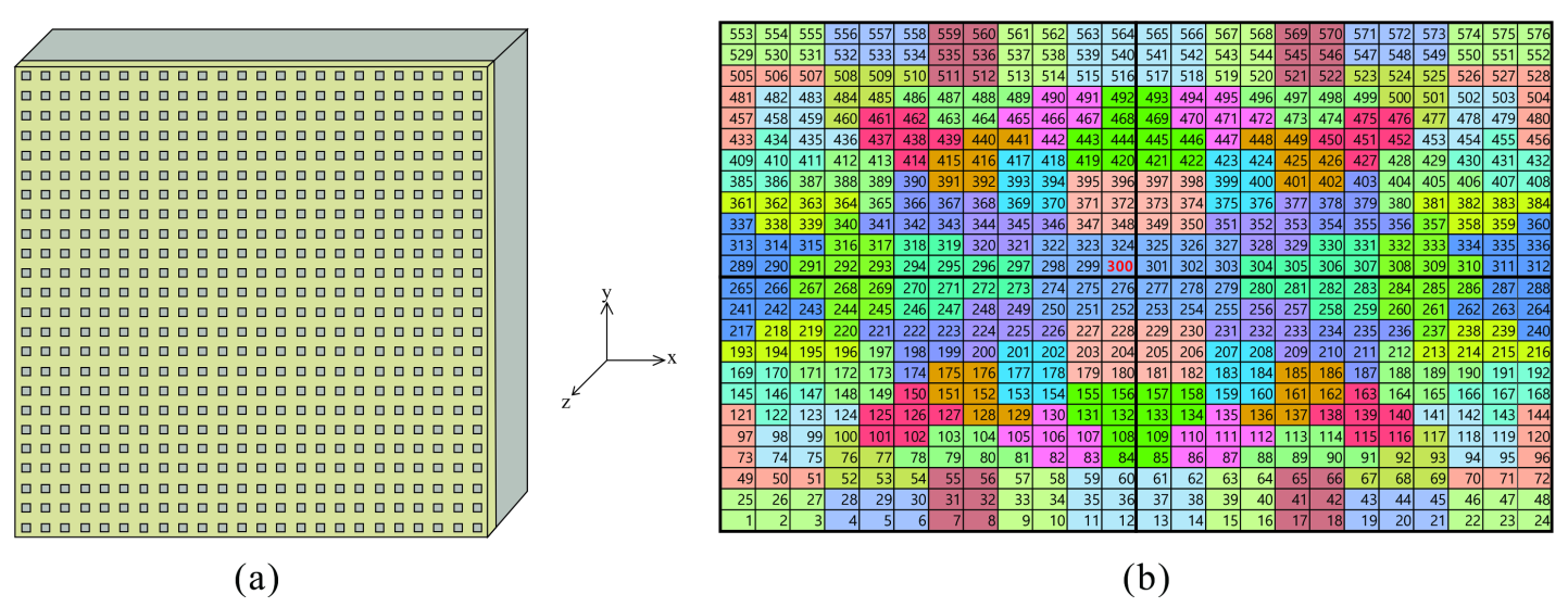
- Design of a 24 × 24 phased array antenna with uniform weighting.
- Step2.
- Arbitrarily allocate the phase centers to any points on the array antenna in the first quadrant.
- Step3.
- Shape the subarray by clustering the radiating elements based on the assigned phase centers.
- Step4.
- Place an origin symmetry on the optimized subarray formed in the first quadrant of the array antenna.
- Step5.
- Check the grating lobe by calculating (Equation (1)) on the condition of uniform weighting ().
- Step6.
- If grating lobe takes place, repeat Step 2–5.
- Step7.
- Step8.
- Calculate the SLL from (Equation (1)), applying optimized weighting derived by QP.
- Step9.
- If the SLL is not satisfied, repeat Step 2–8 by reshaping the subarray or updating phase centers until the last iteration of GSO.
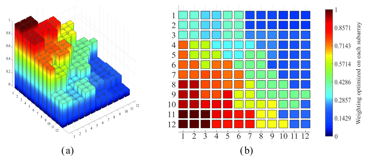
2.2. Weighting Optimized by Quadratic Programming
2.3. Analysis of Subarray Weighting Optimization
3. Calculation of the Array Pattern with Optimized Weighting Applied to Each Subarray Considering Mutual Coupling
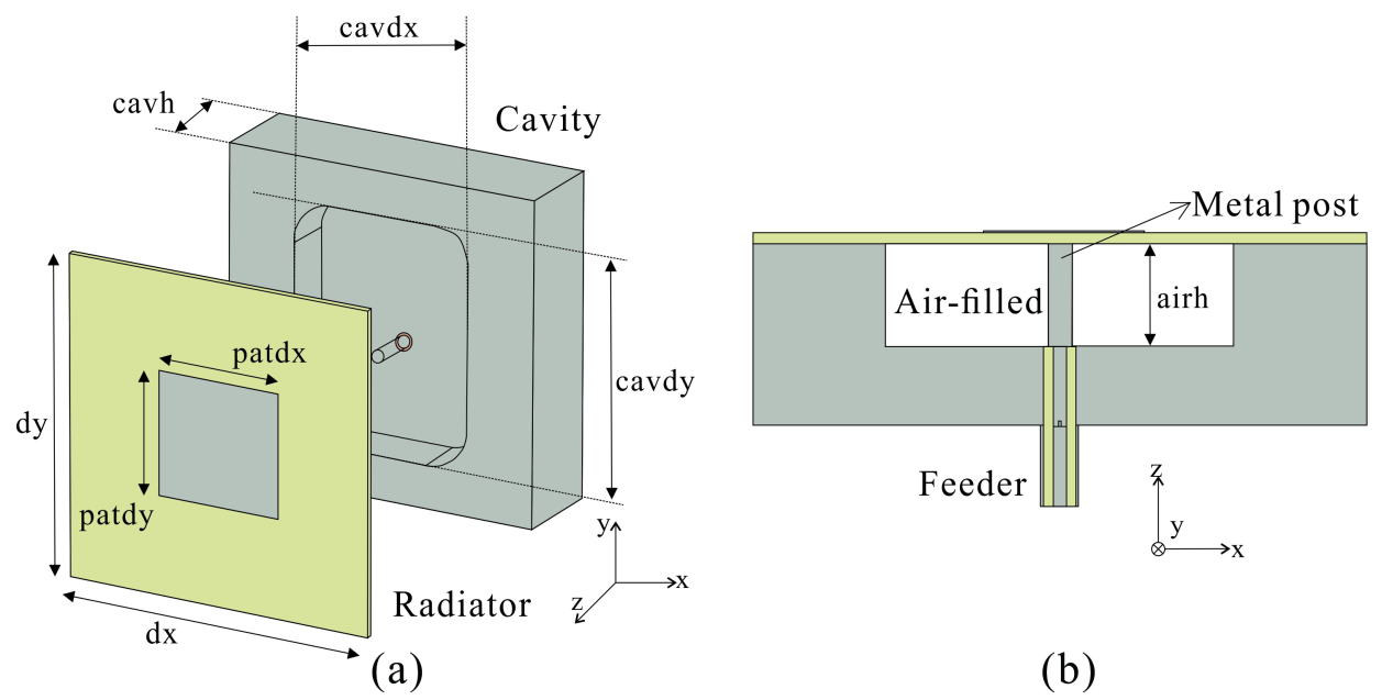
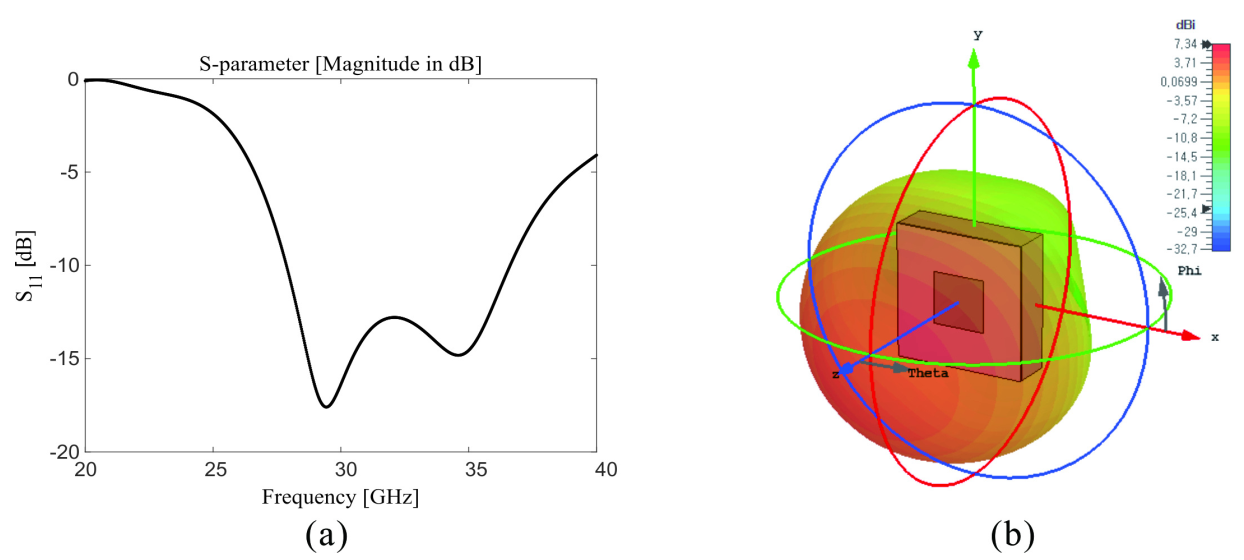
3.1. Cavity-Backed Type Single Radiating Element Design and mm-Wave Analysis
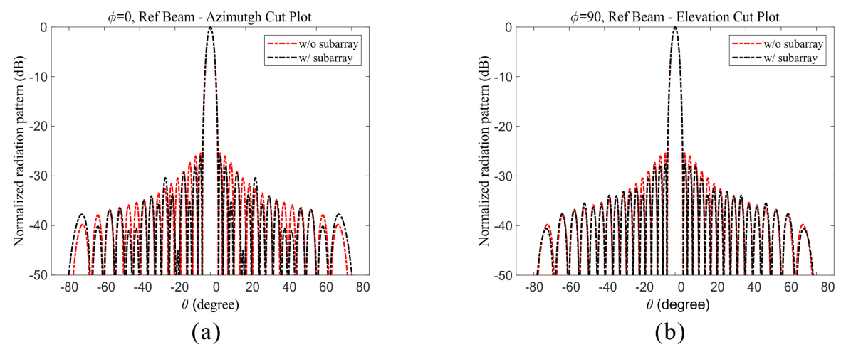
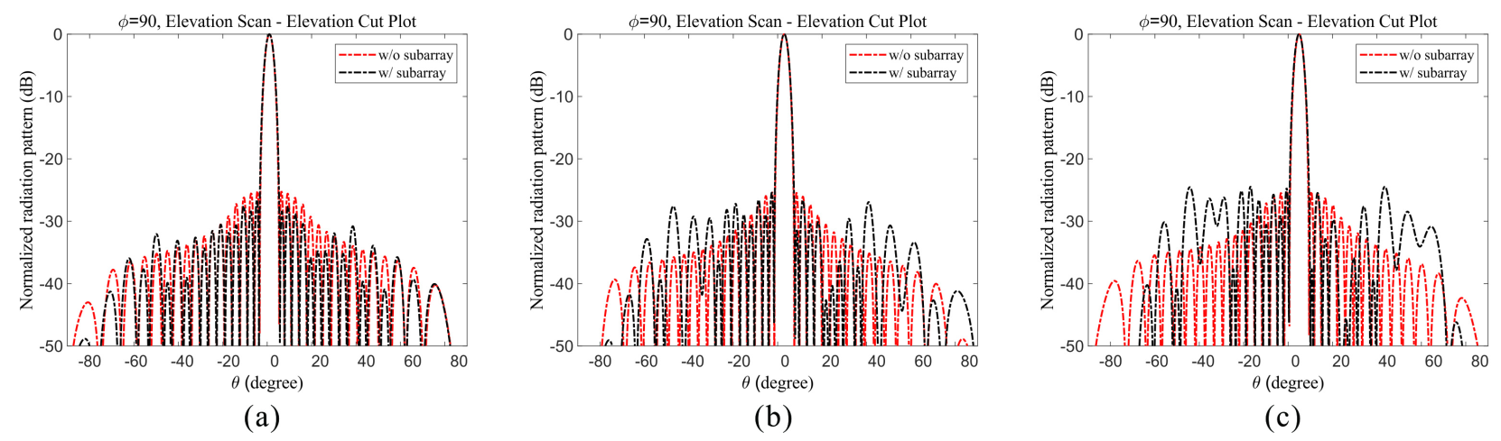
3.2. Array Antenna Design and Calculation of an Array Pattern Considering Mutual Coupling
4. Conclusions
Author Contributions
Funding
Institutional Review Board Statement
Informed Consent Statement
Data Availability Statement
Conflicts of Interest
References
- Nickel, U.R. Properties of digital beamforming with subarrays. IEEE Aerosp. Electron. Syst. Mag. 2006, 20, 46. [Google Scholar]
- Sarkar, T.K.; Mailloux, R.J. A History of Phased Array Antennas, in History of Wireless; John Wiley & Sons, Inc.: Hoboken, NJ, USA, 2006. [Google Scholar]
- Mailloux, R.J. A low-sidelobe partially overlapped constrained feed network for time-delayed subarrays. IEEE Trans. Antennas Propag. 2001, 49, 280–291. [Google Scholar] [CrossRef]
- Hall, P.S.; Smith, M.S. Sequentially rotated arrays with reduced sidelobe levels. IEE Proc. Microw. Antennas Propag. 1994, 141, 321–325. [Google Scholar] [CrossRef]
- Toyama, N. Aperiodic array consisting of subarrays for use in small mobile earth stations. IEEE Trans. Antennas Propag. 2005, 53, 2004–2010. [Google Scholar] [CrossRef]
- Haupt, R.L. Optimized weighting of uniform subarrays of unequal sizes. IEEE Trans. Antennas Propag. 2007, 53, 1207–1210. [Google Scholar] [CrossRef]
- Lee, H.; Boo, S.; Kim, G.; Lee, B. Optimization of excitation magnitudes and phases for maximum efficiencies in a MISO wireless power transfer system. J. Electromagn. Eng. Sci. 2020, 20, 16–22. [Google Scholar] [CrossRef]
- Hur, J.; Choo, H. Design of a Small Array Antenna with an Extended Cavity Structure for Wireless Power Transmission. J. Electromagn. Eng. Sci. 2020, 20, 9–15. [Google Scholar] [CrossRef]
- Nguyen, T.K.; Lee, I.; Kwon, O.; Kim, Y.J.; Hong, I. Metaheuristic Optimization Techniques for an Electromagnetic Multilayer Radome Design. J. Electromagn. Eng. Sci. 2019, 19, 31–36. [Google Scholar] [CrossRef]
- Choi, I.; Jung, J.; Kim, K.; Park, S. Novel Parameter Estimation Method for a Ballistic Warhead with Micromotion. J. Electromagn. Eng. Sci. 2020, 20, 262–269. [Google Scholar] [CrossRef]
- Yang, K.; Wang, Y.; Tang, H. A subarray design method for low sidelobe levels. Prog. Electromagn. Res. Lett. 2020, 48, 45–51. [Google Scholar] [CrossRef]
- Fuchs, B.; Fuchs, J.J. Optimal Narrow Beam Low Sidelobe Synthesis for Arbitrary Arrays. IEEE Trans. Antennas Propag. 2010, 58, 2130–2135. [Google Scholar] [CrossRef]
- Fuchs, B. Shaped Beam Synthesis of Arbitrary Arrays via Linear Programming. IEEE Antennas Wirel. Propag. Lett. 2010, 9, 481–484. [Google Scholar] [CrossRef]
- Manica, L.; Rocca, P.; Massa, A. Design of Subarrayed Linear and Planar Array Antennas with SLL Control Based on an Excitation Matching Approach. IEEE Trans. Antennas Propag. 2009, 57, 1684–1691. [Google Scholar] [CrossRef]
- Mailloux, R.J.; Santarelli, S.G.; Roberts, D.L.; Luu, D. Irregular Polyomino-Shaped Subarrays for Space-Based Active Arrays. Int. J. Antennas Propag. 2009. [Google Scholar] [CrossRef]
- Rocca, P.; Oliveri, G.; Mailloux, R.J.; Massa, A. Unconventional Phased Array Architectures and Design Methodologies—A Review. IEEE Proc. 2016, 104, 544–560. [Google Scholar] [CrossRef]
- Jang, D.; Hur, J.; Shim, H.; Park, J.; Cho, C.; Choo, H. Array Antenna Design for Passive Coherent Location Systems with Non-Uniform Array Configurations. J. Electromagn. Eng. Sci. 2020, 20, 176–182. [Google Scholar] [CrossRef]
- Haupt, R.L. Antenna Arrays—A Computation Approach; Wiley-IEEE Press: Hoboken, NJ, USA, 2010. [Google Scholar]
- Bevelacqua, P.J. Antenna Arrays: Performance Limits and Geometry Optimization. Ph.D. Thesis, School of Electrical, Computer and Energy Engineering, Arizona State University, Tempe, AZ, USA, 2008. [Google Scholar]
- Nickel, U.R. Subarray configurations for digital beamforming with low sidelobes and adaptive interference suppression. In Proceedings of the International Conference on Radar, Alexandria, VA, USA, 8–11 May 1995; pp. 714–719. [Google Scholar]
- Haupt, R.L. Reducing grating lobes due to subarray amplitude tapering. IEEE Trans. Antennas Propag. 1985, 33, 846–850. [Google Scholar] [CrossRef]
- Şeker, I. Calibration methods for phased array radars. Proc. SPIE 2013, 8714, 87140W. [Google Scholar]
- Kwon, G.; Park, J.Y.; Hwang, K.C. Design of a subarray configuration for multifunction radars using a nested optimization scheme. Electromagnetics 2016, 5, 276–285. [Google Scholar] [CrossRef]
- Hansen, R.C. Phased Array Antennas, 2nd ed.; John Wiley & Sons, Inc.: Hoboken, NJ, USA, 2009. [Google Scholar]
- Kwon, G.; Park, J.; Kim, D.; Hwang, K.C. Optimization of a shared-aperture dual-band transmitting/receiving array antenna for radar applications. IEEE Trans. Antennas Propag. 2017, 65, 7038–7051. [Google Scholar] [CrossRef]
- MATLAB Documentation of Quadprog Function. Available online: http://www.mathworks.com/help/optim/ug/quadprog.html (accessed on 30 April 2021).
- Bhattacharyya, A.K. Phased Array Antennas; John Wiley & Sons, Inc.: Hoboken, NJ, USA, 2006. [Google Scholar]


| Azimuth Scan (Azimuth Cut Plot) | Elevation Scan (Elevation Cut Plot) | |||
|---|---|---|---|---|
| w/a Subarray | w/o a Subarray | w/a Subarray | w/o a Subarray | |
| Boresight | −26.18 dB/3.6 | −25.38 dB/3.6 | −27.36 dB/3.6 | −25.38 dB/3.6 |
| 1 scanning | −25.68 dB/3.6 | −25.19 dB/3.6 | −26.58 dB/3.6 | −25.19 dB/3.6 |
| 3 scanning | −24.83 dB/3.6 | −25.36 dB/3.6 | −25.42 dB/3.6 | −25.36 dB/3.6 |
| 5 scanning | −22.87 dB/3.7 | −25.17 dB/3.7 | −24.50 dB/3.7 | −25.17 dB/3.7 |
| Parameter | Value | Parameter | Value |
|---|---|---|---|
| dx | 7.2 | cavh | 2.12 |
| dy | 7.2 | cavdx | 4.11 |
| patdx | 2.9 | cavdy | 5.31 |
| patdy | 2.8 | airh | 1.21 |
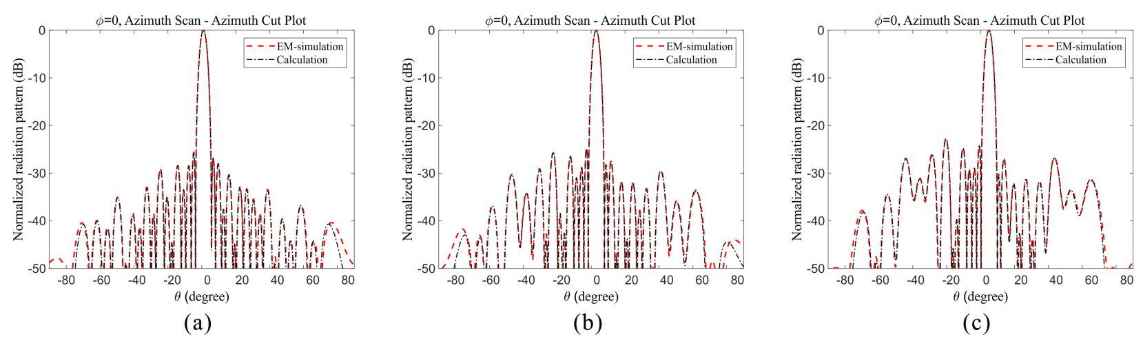
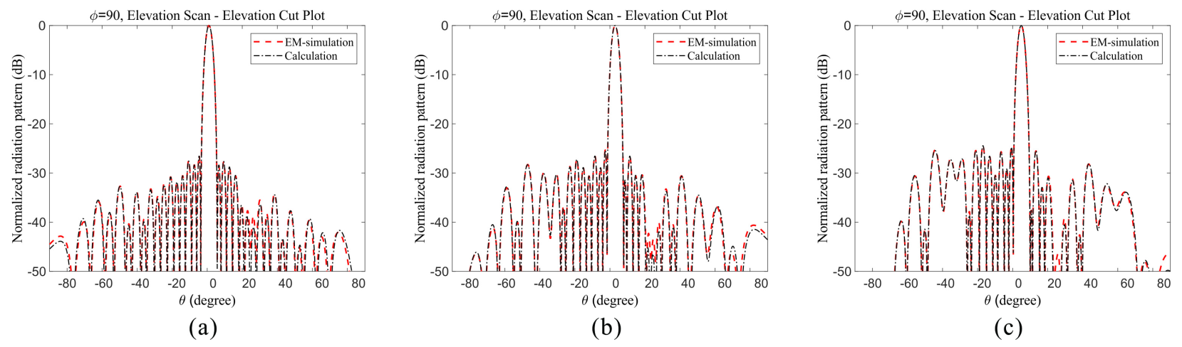
| Azimuth Scan (Azimuth Cut Plot) | Elevation Scan (Elevation Cut Plot) | |||
|---|---|---|---|---|
| Calc. | EM-Sim. | Calc. | EM-Sim. | |
| Boresight | −26.21 dB/3.6 | −25.38 dB/3.6 | −27.39 dB/3.6 | −25.38 dB/3.6 |
| 1 scanning | −25.68 dB/3.6 | −25.61 dB/3.6 | −26.58 dB/3.6 | −26.51 dB/3.6 |
| 3 scanning | −24.87 dB/3.6 | −24.78 dB/3.6 | −25.40 dB/3.6 | −25.33 dB/3.6 |
| 5 scanning | −22.70 dB/3.7 | −22.86 dB/3.7 | −24.44 dB/3.7 | −24.49 dB/3.7 |
Publisher’s Note: MDPI stays neutral with regard to jurisdictional claims in published maps and institutional affiliations. |
© 2021 by the authors. Licensee MDPI, Basel, Switzerland. This article is an open access article distributed under the terms and conditions of the Creative Commons Attribution (CC BY) license (https://creativecommons.org/licenses/by/4.0/).
Share and Cite
Jeong, T.; Yun, J.; Oh, K.; Kim, J.; Woo, D.W.; Hwang, K.C. Shape and Weighting Optimization of a Subarray for an mm-Wave Phased Array Antenna. Appl. Sci. 2021, 11, 6803. https://doi.org/10.3390/app11156803
Jeong T, Yun J, Oh K, Kim J, Woo DW, Hwang KC. Shape and Weighting Optimization of a Subarray for an mm-Wave Phased Array Antenna. Applied Sciences. 2021; 11(15):6803. https://doi.org/10.3390/app11156803
Chicago/Turabian StyleJeong, Taeyong, Juho Yun, Kyunghyun Oh, Jihyung Kim, Dae Woong Woo, and Keum Cheol Hwang. 2021. "Shape and Weighting Optimization of a Subarray for an mm-Wave Phased Array Antenna" Applied Sciences 11, no. 15: 6803. https://doi.org/10.3390/app11156803
APA StyleJeong, T., Yun, J., Oh, K., Kim, J., Woo, D. W., & Hwang, K. C. (2021). Shape and Weighting Optimization of a Subarray for an mm-Wave Phased Array Antenna. Applied Sciences, 11(15), 6803. https://doi.org/10.3390/app11156803