A New Characterization Method for Rock Joint Roughness Considering the Mechanical Contribution of Each Asperity Order

Abstract

The morphology of the joint surface is multi-scale, and it can be divided into first-order asperity (waviness) and second-order asperity (unevenness). At present, the joint roughness characterization formula considers only the morphology contribution of waviness and unevenness components and does not fully consider their mechanical contribution. At same time, the relationship between the mechanical contribution and the morphology contribution is still unclear. Thus, the characterization formula considering the mechanical contribution of waviness and unevenness needs to be further studied. In this study, the standard joint roughness coefficient (JRC) profiles were first decomposed into waviness and unevenness. Then, three types of joint specimens with different asperity orders (flat, the standard JRC profile, and the profile containing only waviness) were prepared by the 3D engraving technique. Finally, direct shear tests were carried out on 39 sets of red sandstone joint specimens under three normal stresses. The mechanical contributions of waviness and unevenness were studied, the relationship between the mechanical contribution and the morphology contribution of waviness and unevenness was analyzed, and the characterization formula considering the mechanical contribution of waviness and unevenness was established. The results showed that the following: (1) the method combining the ensemble empirical mode decomposition (EEMD) and the critical decomposition level could be used to separate the waviness and unevenness from the joint surface; (2) the mechanical contribution of the waviness and unevenness decreased with the increase in normal stress; (3) the relationship between the mechanical contribution ratio and the statistical parameter ratio of the waviness and unevenness can be describe by power function; and (4) the roughness characterization formula considering the mechanical contribution and morphology contribution was established. This study will enhance the accurate evaluation of the roughness coefficient and shear strength of the joint specimen.

1. Introduction

Rock mass contains a large number of discontinuities, such as joints, faults, bedding planes, or any other planar defects. These discontinuities play a weakening role in the rock mass. Under low normal stress, rock mass behavior is controlled by sliding along existing discontinuities rather than failure of the intact rock material [1]. Thus, the shear behavior of rock joints plays a key role in the safety and stability of underground mining [2,3,4,5,6]. The roughness of rock joints is recognized as one of the most important parameters affecting mechanical behavior [7,8,9,10,11]. Thus, quantitative characterization of discontinuity roughness has recently become a research hotspot in the field of rock mechanics.

In 1973, Barton [12] first proposed a concept called the joint roughness coefficient (JRC) to describe the joint surface morphology. In 1977, Barton and Choubey [13] proposed a method whereby the roughness of the joint specimen could be determined by visual comparison. This method was suggested by the International Society for Rock Mechanics (ISRM) [14] and is currently used in engineering applications. However, this method was proven to be subjective [15,16] and affected by the experience of the engineer [17]. In order to quantify joint surface roughness objectively, a series of objective quantification methods by statistical parameters were gradually proposed. Tse [18] first calculated the type-profiles’ statistical parameters and correlated them with the JRC. Then, a series of statistical parameters (Z₂, R_P, SF, Z_2s, ${\theta }_{\max }^{\ast }/\left(C+1\right)$ [19]) were proposed to describe joint roughness in two and three dimensions, and characterization formulas were established based on these statistical parameters. The statistical parameters and the formulas are shown in

Table 1. The statistical parameter and characterization formula by single parameter.

Parameter	Formula	Ref.
$Z_2={\left[\frac{1}{L}{\displaystyle \sum _{i=1}^{n-1}\frac{{\left(y_{i+1}-y_i\right)}^2}{x_{i+1}-x_i}}\right]}^{1/2}$	$\begin{array}{c}JRC=32.2+32.47\log Z_2\\ JRC=130.87{(Z_2)}^2-2.73\\ JRC=32.69+32.98\lg Z_2\\ JRC=51.85Z_2^{0.6}-10.37\\ JRC=51.16Z_2^{20.531}-11.44\\ JRC=55.7376Z_2-4.1166\\ JRC=32.172\log Z_2+32.202\\ JRC=57.82{[1-b(Z_2)]}^{-0.26}\sqrt{a\left(Z_2\right)}-13.5\end{array}$	[18] [20] [21] [22] [23] [24] [25] [26]
$SF=\frac{1}{L}{\displaystyle \sum _{i=1}^{n-1}{\left(y_{i+1}-y_i\right)}^2\left(x_{i+1}-x_i\right)}$	$\begin{array}{c}JRC=37.28+16.58\log SF\\ JRC=16.67\log (SF)+37.726\\ JRC=-3.28+121.13\sqrt{SF}\\ JRC=37.63+16.5\log (SF)\\ JRC=73.95{(SF)}^{0.266}-11.38\end{array}$	[18] [20] [21] [23] [25]
$R_P=\left(L_t-L\right)/L$	$\begin{array}{c}JRC=77.06{(R_P-1)}^{0.172}-29.27\\ JRC=47.62+93.74{(R_P-1)}^{0.1235}\\ JRC=63.69\sqrt{R_P-1}-2.31\\ JRC={\left(0.036+\frac{0.00127}{\ln (R_P)}\right)}^{-1}\\ JRC=411\left(R_P-1\right)\\ JRC=65.9{(R_P-1)}^{0.302}-9.65\end{array}$	[21] [22] [23] [25] [27] [28]
${\theta }_{p^{+}}={\tan }^{-1}\left\{\frac{1}{M_{x^{+}}}{\displaystyle \sum _{i=1}^{M_{x^{+}}}{\left[{\left(\frac{y_{i+1}-y_i}{x_{i+1}-x_i}\right)}_{+}\right]}_i}\right\}$ [29]	$JRC=-106.67{({\theta }_{p^{+}})}^{-0.363}+55.34$	[30]
$Z_2^{\prime }={\left[\frac{1}{M{\left(\Delta x\right)}^2}{\displaystyle \sum _{i=1}^M{\left(\max (0,y_{i+1}-y_i)\right)}^2}\right]}^{1/2}$ [31]	$JRC=-9.43{(Z_2^{\prime })}^{-0.687}+35.11$	[30]
$\begin{array}{c}\tan {\theta }^{\ast }=-\tan \theta \cos \alpha \\ A_{{\theta }^{\ast }}=A_0{\left(\frac{{\theta }_{\max }^{\ast }-{\theta }^{\ast }}{{\theta }_{\max }^{\ast }}\right)}^C\end{array}$ [32]	$JRC=3.95{\left({\theta }_{\max }^{\ast }/\left[C+1\right]\right)}_{2D}{}^{0.7}-7.98$	[22]
$r_i=\frac{A_i}{{\displaystyle \sum _{i=1}^n{A}_i}},R_i={\theta }_i^{\ast }{r}_i,WPA={\displaystyle \sum _{i=1}^{i=m}{R}_i^{+}}$ [33]	$JRC=14.602\ln \left(WPA\right)-12.536$	[33]

.

With the development of scanning technology, three-dimensional (3D) statistical parameters were proposed. Based on the “local apparent inclination asperity dip”, a 3D roughness parameter was proposed [32,34,35,36]. In addition, the joint roughness was studied from the perspective of a power spectrum [37,38]. Although increasing attention has been given to 3D characterization of fracture surface roughness in recent years, the characterization of linear profiles remains important for applications. The morphology of the joint specimen is complex and multi-scale [39,40,41,42,43]. The ISRM has divided the morphology into primary asperity (waviness) and secondary asperity (unevenness). At the same time, the contributions of different orders of asperity to the shear strength are different [44,45,46,47]. The joint roughness would be underestimated if it were characterized by a single statistical parameter [48]. In order to solve this problem, multiple joint roughness formulas characterized by two parameters have been proposed, as shown in

Table 2. The characterization formula by two statistical parameters.

Formula	Ref.
$JRC=1979R_d^{0.92}{\epsilon }^{1.46}$	[49]
$JRC=15179W_d^{0.79}{(D-1)}^{1.46}$	[50]
$\begin{array}{c}JRC=12.862R+10.316\arctan (100R_a)-4.017\hspace{0.33em}\hspace{0.33em}\\ JRC=2.719R+0.585\arctan {(100R_a)}^2+6.169\hspace{0.33em}\\ JRC=10.544R+0.327\arctan {(100R_a)}^2+10.377\hspace{0.33em}\end{array}$	[51]
$\begin{array}{c}JRC=41.14\log \left(Z_2\right)+4.93A_{\mathrm{nor}}^{1.53}+26.72\hspace{0.33em}\\ JRC=33.86\log \left(Z_2\right)+3.19A_{\mathrm{nor}}^{2.02}+28.92\hspace{0.33em}\\ JRC=26.31\log \left(Z_2\right)+2.20A_{\mathrm{nor}}^{2.12}+27.73\end{array}$	[52]
$\begin{array}{c}JRC=69.23\sqrt{Z_2}-28.17h_A^{-0.03}\hspace{0.33em}\\ JRC=64.75\sqrt{Z_2}-20.45h_A^{-0.11}\hspace{0.33em}\\ JRC=58.92\sqrt{Z_2}-15.74h_A^{-0.06}\hspace{0.33em}\\ JRC=57.62\sqrt{Z_2}-13.73h_A^{0.08}\hspace{0.33em}\hspace{0.33em}\hspace{0.33em}\end{array}$	[53]
$\begin{array}{c}JRC=75.11Z_2^{1\mathrm{st}}+3.33Z_2^{2\mathrm{nd}}-2.79\hspace{0.33em}\\ JRC=91.73S{F}^{1\mathrm{st}}-57.13S{F}^{2\mathrm{nd}}+3.89\hspace{0.33em}\\ JRC=472.16{(R_P-1)}^{1\mathrm{st}}-20.42{\left(R_P-1\right)}^{2\mathrm{nd}}+3.32\end{array}$	[54]
$\begin{array}{c}JRC=A\times {\displaystyle \sum {\left(S_{up}^{2\mathrm{nd}}\right)}^a+B\times {\displaystyle \sum {\left(S_{up}^{1\mathrm{st}}\right)}^b+C}}\\ JRC=A\times {\displaystyle \sum {\left(V_{up}^{2\mathrm{nd}}\right)}^a+B\times {\displaystyle \sum {\left(V_{up}^{1\mathrm{st}}\right)}^b+C}}\end{array}$	[55]
$\begin{array}{c}JRC=1.2{\theta }_{2d}+867.5h_1^2-2.9\\ {\theta }_{2d}={\left[{\theta }_{\max }^{\ast }/\left(C+1\right)\right]}_{2d}\\ h_1=h/L\end{array}$	[9]

. However, the parameters proposed by previous researchers ([9,49,50,51,52,53]) do not quantify waviness and unevenness. Liu et al. [54,55] characterized joint roughness with two statistical parameters by decomposing the joint surface into waviness and unevenness. However, this formula considers only the morphology contribution, and not the full mechanical contribution.

At present, several methods, such as the Fourier series method [56,57,58,59,60], different sampling interval methods [61,62,63,64], and the wavelet analysis method [65], are used for the separation of waviness and unevenness from the joint surface. However, these methods are limited by the characteristics of themselves [66]. The Fourier series method [67] and wavelet analysis both need a priori function, and this function will affect the final result. At the same time, a variety of methods have been proposed to identify waviness and unevenness. Yang [56] proposed a method to distinguish waviness and unevenness by visual observation. Ficker [61] proposed distinguishing waviness and unevenness through the change law of joint surface area at different sampling intervals. Zou [65] proposed a law to identify the cut-off level by the variance law of the approximate component. However, a method with clear mathematical definition to judge the critical decomposition level has not yet been proposed.

In summary, the morphology of the joint specimen is multi-scale. The joint roughness will be underestimated if it is characterized by a single statistical parameter. At same time, the mechanical contribution and the morphology contribution of each asperity order are different. At present, the joint surface roughness characterization formula considers only the morphology contribution of the waviness and unevenness, and not their full mechanical contribution. In this study, the standard JRC profiles were taken as the initial morphology and were decomposed into waviness and unevenness by the method combining the ensemble empirical mode decomposition (EEMD) and the criterion of critical decomposition level. Three types of joint specimens with different asperity orders were prepared with the 3D carving method. Shear tests were carried out on 39 groups of red sandstone joint specimens with seven roughness degrees (5^#~10^# standard JRC profiles and flat joint planes) and two asperity orders (one including only waviness and one including waviness and unevenness) under three normal stresses. The mechanical contribution of each asperity order was analyzed, and the relationship between the mechanical contribution of each asperity order and its statistical parameter was explored. Finally, the characterization formula of joint roughness that considers the mechanical contribution of each asperity was established.

2. Decomposition of the Standard JRC Profile

In the field of mathematics, any complex curve can be regarded as a superposition of sine waves and cosine waves (partial waves) of different wavelengths and amplitudes [38]. The standard JRC profile is no exception. Empirical Mode Decomposition (EMD) has been widely used in the trend item extraction of signals [68]. This method does not require any prior knowledge in its application and is suitable for various types of signals.

2.1. Standard JRC Profile Decomposition Method

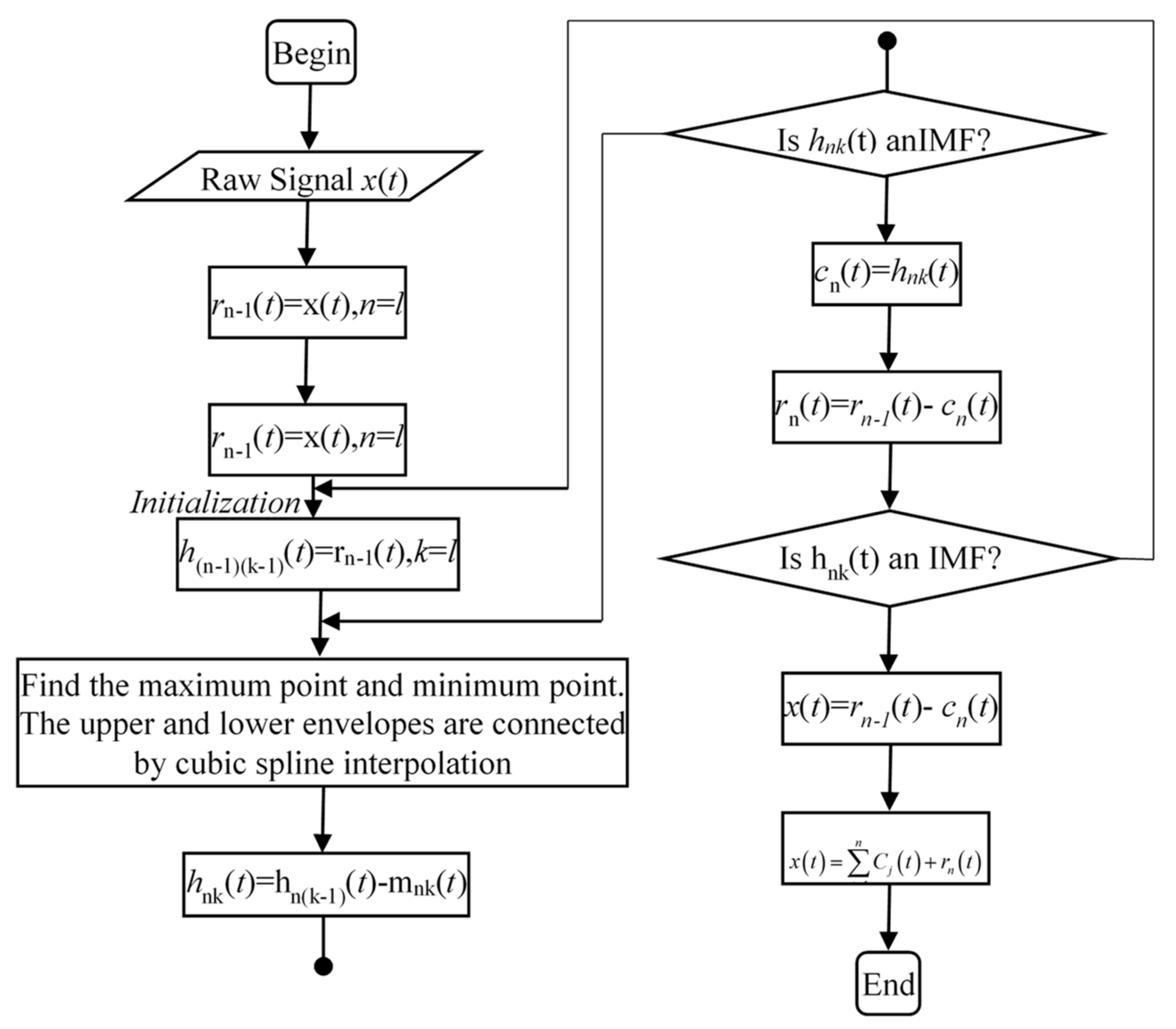
2.1.1. Empirical Mode Decomposition Method

Empirical Mode Decomposition (EMD) is a signal decomposition method based on the characteristic timescale of the signal itself. It does not need a fixed a priori basis function, and it is self-adaptive. It decomposes the fluctuation or trend at different scales in the signal, step by step, and generates a series of data sequences with different characteristic scales, namely, the intrinsic mode function (IMF).

IMF is a function satisfying the following two conditions [69]:

(1)

In the entire data set, the number of crossing zero points and extreme value points is the same or the difference between them is 1;

(2)

At any point on the signal, the mean value of the upper envelope defined by the local maximum and the lower envelope defined by the local minimum are 0, which means that the signal is locally symmetric about the time axis.

The following three assumptions need to be satisfied when the EMD method is used to signal decomposition:

(1)

The signal has at least two extreme points: a maximum point and a minimum point;

(2)

The characteristic timescale is defined as the time interval between adjacent extreme points;

(3)

If the signal does not have an extreme point and has only an inflection point, it should be differentiated one or more times to obtain the extremum point before decomposition, and then the corresponding component can be obtained by integrating the obtained result.

EMD is a method of decomposing signals through the sifting process. The sifting process can be divided into three steps:

Step 1: First, determine all extreme points for a target signal X(t). The upper envelope is obtained by connecting all the maximum points with a cubic spline function, and the lower envelope is obtained by connecting all the minimum points with a cubic spline function. The difference between the signal X(t) and the mean of the upper and lower envelopes is denoted as h₁, as follows:

$$h_1=X-\left(E^{+}\left(t\right)+E^{-}\left(t\right)\right)/2$$

(1)

Then, h₁ is regarded as the new X(t), and Step 1 is repeated until h_i meets the two limiting conditions of the IMF; the first-order IMF, called IMF₁, is then sieved from the signal.

Step 2: Separate IMF1 from X(t) to obtain a different signal called RES₁ with the IMF₁ component removed.

$$RE{S}_1=X\left(t\right)-IM{F}_1$$

(2)

RES₁ is taken as a new signal, and Step 1 is repeated until the n^th order residual sequence (RES_n) becomes a monotone function, and the IMF component cannot be further sieved.

$$RE{S}_n=RE{S}_{n-1}-IM{F}_n$$

(3)

Step 3: From a mathematical perspective, regard the initial signal X(t) as the sum of the IMF component and residual component RES [42]:

$$X\left(t\right)={\displaystyle {\sum }_{i=1}^{n}IM{F}_i+RE{S}_i}$$

(4)

where IMF_i represents the detail component, and RES_i represents the approximate component.

Its flowchart is shown in Figure 1 [70].

2.1.2. Ensemble Empirical Mode Decomposition (EEMD)

In the application of EMD, we see the mode mixing defined as the characteristic component of different timescales decomposed into one IMF, or the same timescale component appearing in different IMFs. The mode mixing causes the IMF component to lose its original single characteristic scale, forming a mixed-scale oscillation. In order to avoid the phenomenon of mode mixing, the EEMD is proposed to decompose the signal. The EEMD takes advantage of the uniform distribution of the white noise spectrum, adding white noise to the signal so that the signals of different time scales can be automatically separated into the corresponding reference scale. As this method mainly supplements missing scales by adding white noise to the signal, it displays good performance in signal decomposition.

The EEMD algorithm processing steps are as follows [71]:

(1)

Adding white noise to the target signal;

(2)

Decomposing the added white noise signal into the IMF;

(3)

Repeating Steps 1 and 2, but adding a different white noise sequence each time;

(4)

Obtaining the mean value of each IMF by decomposition as the final result.

2.1.3. Criterion of Critical Decomposition Level

Accurate decomposition of the waviness and unevenness from the joint surface is the premise for analyzing their mechanical contribution. This is significant to establish the roughness characterization formula which considering their mechanical contribution. The EEMD method only decomposes the standard JRC profile into the approximate component and detail component. In order to obtain the waviness and unevenness from the joint surface, the criterion of critical decomposition level is still needed. According to the qualitative description of waviness by the ISRM, it reflects the macroscopic fluctuation of the joint surface, which contains the main characteristics of the initial standard JRC profile. We speculated that the similarity between the waviness and the initial standard JRC profile would be high. With the increase in decomposition level, more and more detail components are separated from the initial standard JRC profile, which leads to a decrease in the similarity between the approximate components and the initial standard profile. Before reaching the critical decomposition level, the approximate components still contain waviness, and the approximate components can represent the macroscopic fluctuations of the initial standard JRC profile. Therefore, the approximate component has high similarity with the initial standard JRC profile. When the critical decomposition level is exceeded, part of the waviness component is decomposed into the detail component, which suddenly leads to the decrease in similarity between the approximate component and the initial standard JRC profile. Therefore, the similarity between the approximate component and the initial standard JRC profile can be treated as a parameter to determine the critical decomposition level. There are many methods to measure the similarity between two profiles; the cosine similarity criterion was chosen to evaluate the similarity in this study. The unevenness [57] can be regarded as a stationary random process following the Gaussian distribution. The Kolmogorov–Smirnov (K-S) test [72] was chosen to check the distribution characteristics of unevenness at the critical decomposition level.

2.2. Decomposition Result of the Standard JRC Profile

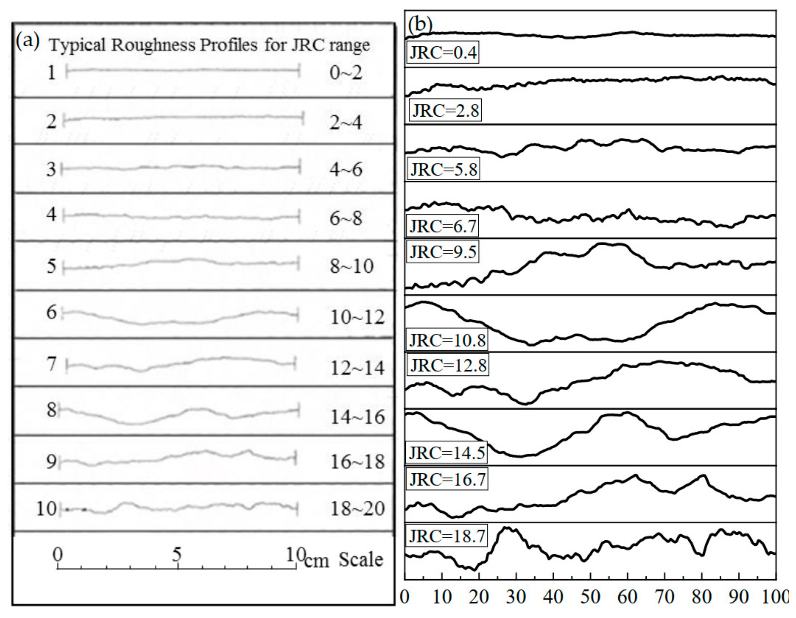
2.2.1. The Digitization Result of the Standard JRC Profile

The standard JRC profile was selected as the initial morphology in this study, and the coordinate value of the standard JRC profile (Figure 2a) was obtained with the gray image processing method [73]. This method results in less error, compared with the data cursor method and the high-resolution scanner method. After obtaining coordinate data, ten standard JRC profiles were reconstructed in Origin software, and the reconstructed results are shown in Figure 2b. By comparing Figure 2a,b, we found that they were basically consistent with each other.

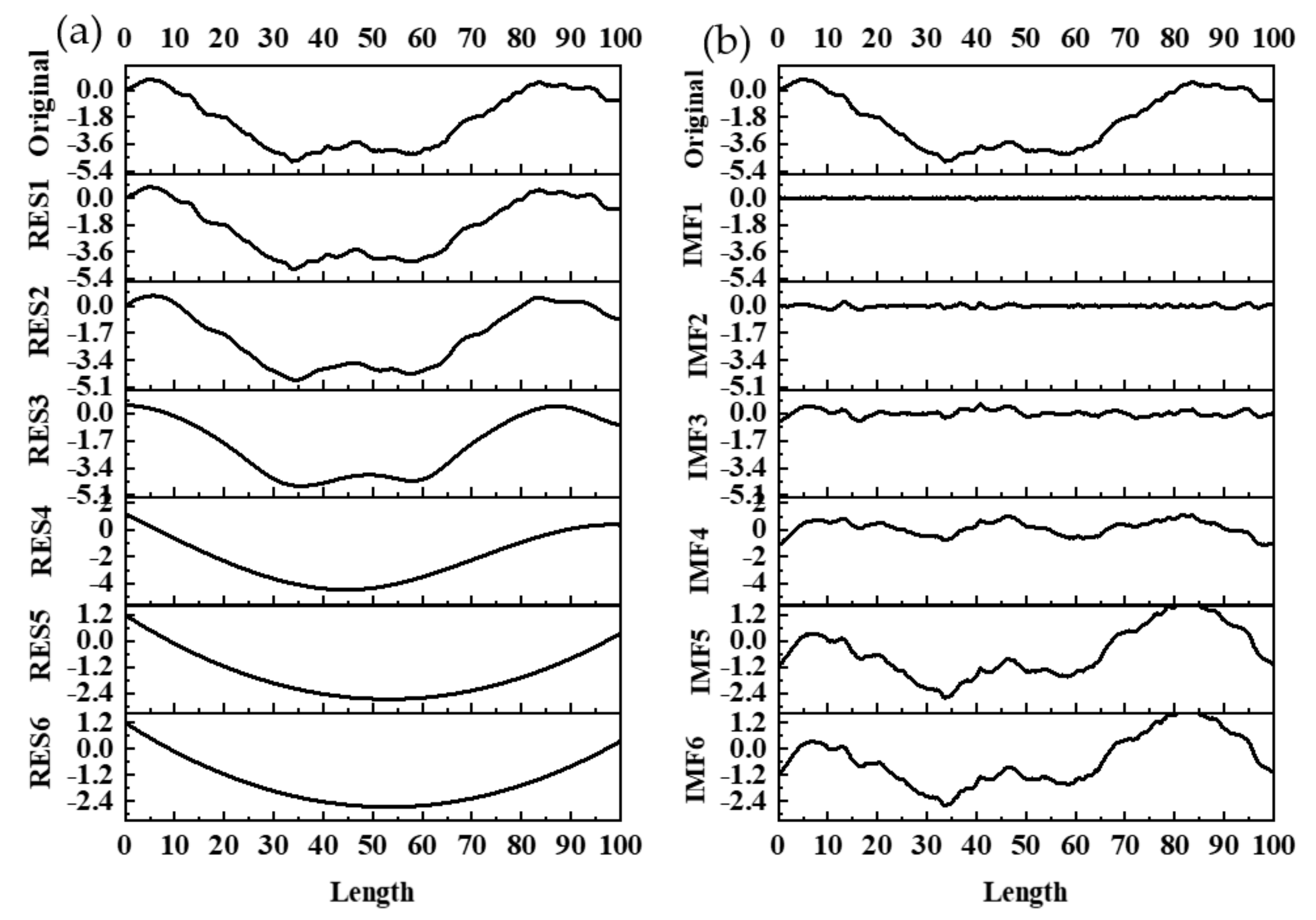
2.2.2. The EEMD Results

The EEMD of ten standard roughness profiles is realized by Matlab software. Figure 3 shows the decomposition result of the 6^# standard JRC profile. The EEMD results of the other standard JRC profiles were similar to this one, so only the decomposition results of the 6^# standard JRC profile are shown here.

The approximate component was characterized by large amplitude and low frequency, which reflected the macroscopic fluctuation of the joint surface, and the detail component showed small-scale fluctuation with small amplitude and high frequency when the decomposition level was lower than 3 (as shown in Figure 3a). With the increase in the decomposition level, some features of the approximate components were extracted as detail components, so the approximate components were no longer able to reflect the macroscopic fluctuation of the joint surface, as shown in Figure 3b.

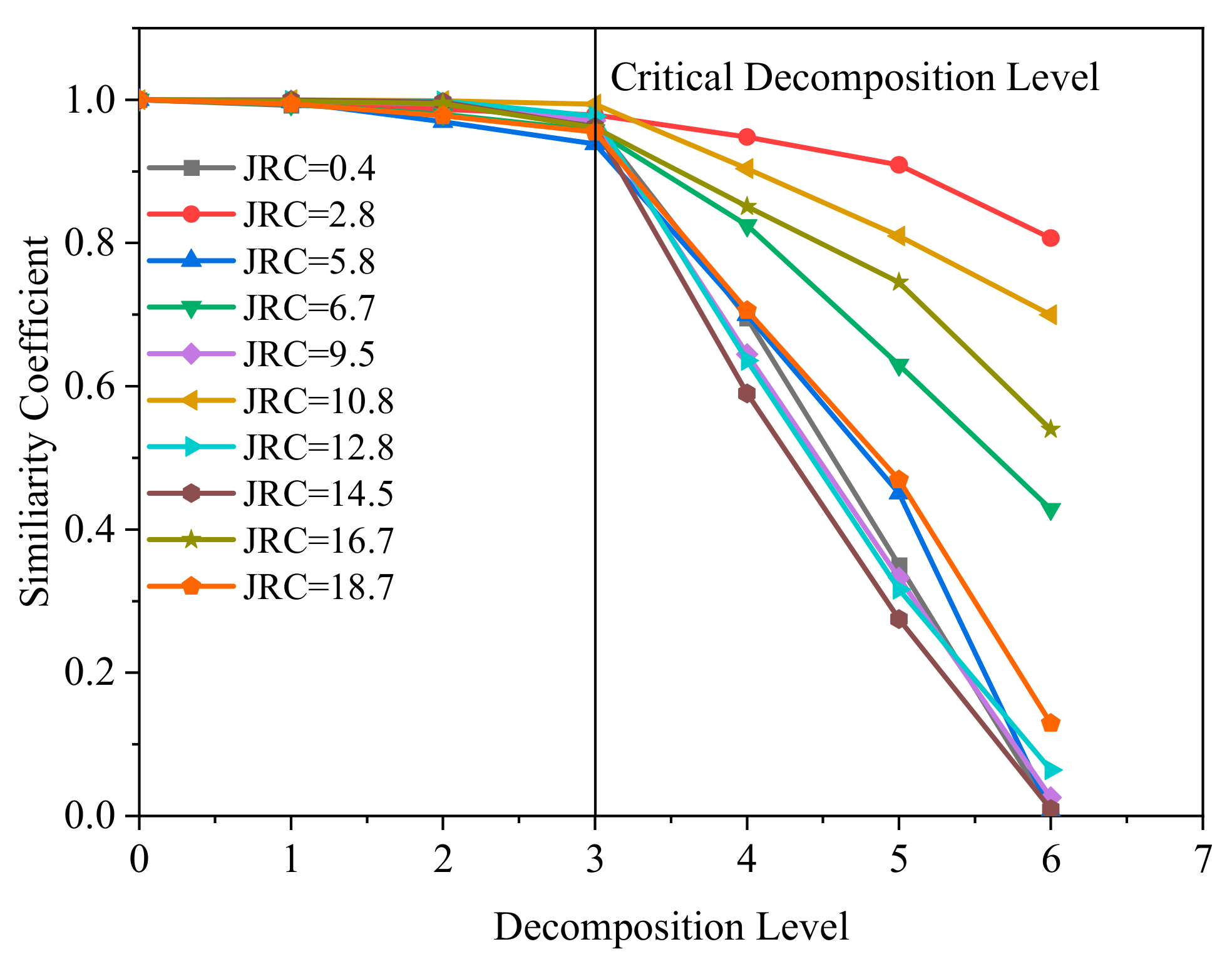
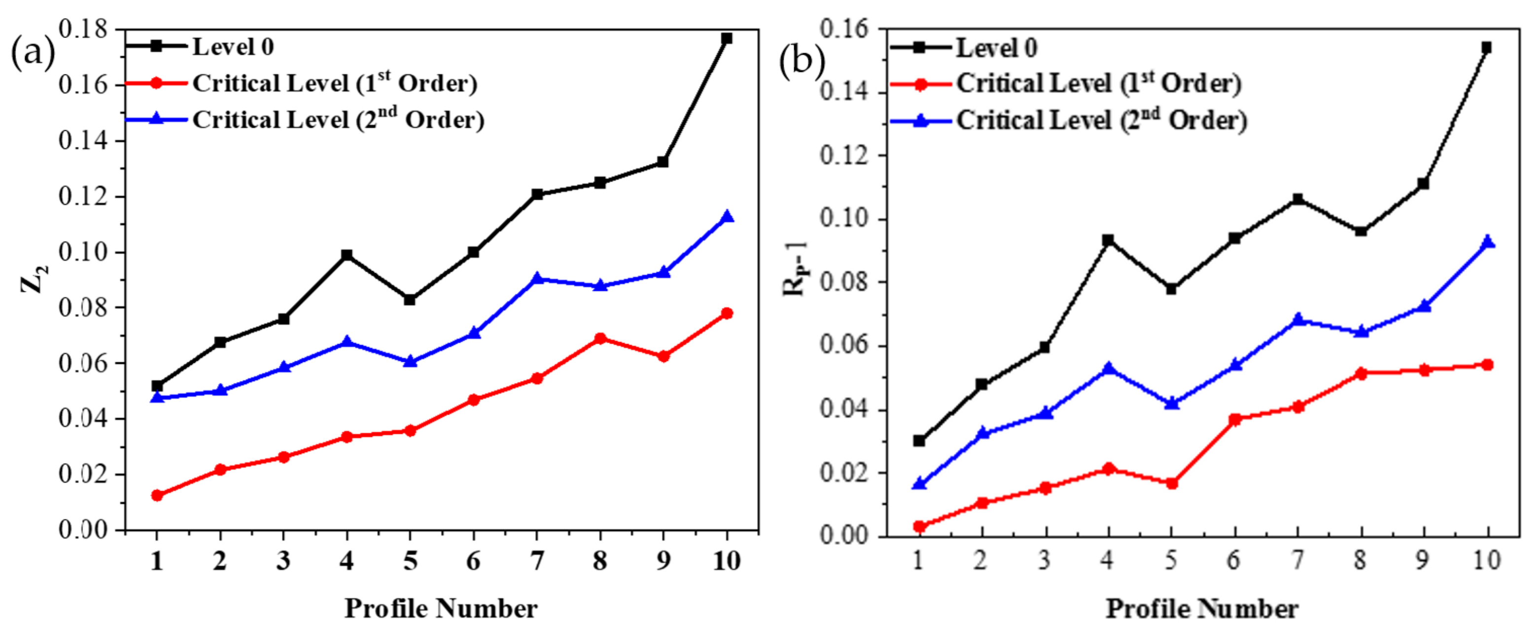
2.2.3. Critical Decomposition Level

In order to determine the critical decomposition level, the similarity between the approximate component and the initial standard JRC profile was calculated, and the calculated results are shown in Figure 4.

The similarity coefficient decreased gradually with the increase in the decomposition level, and the similarity decreased significantly when the decomposition level was large. When the decomposition level was greater than 3, the similarity coefficient began to drop sharply, as shown in Figure 4. Therefore, the 3rd decomposition level was taken as the critical decomposition level; the 3rd level of the approximation component was determined to be the waviness; and the sum of levels 1–3 of the detail components were used to form the unevenness.

The height distribution of the unevenness components was statistically analyzed, and the Kolmogorov–Smirnov (k-s) test was used to check the distribution of the detail components. The statistical results are shown in Figure 5.

The p values of all ten standard JRC profiles were greater than 0.05, as shown in Figure 5. We concluded that the unevenness components of all ten standard JRC profiles met the Gaussian distribution.

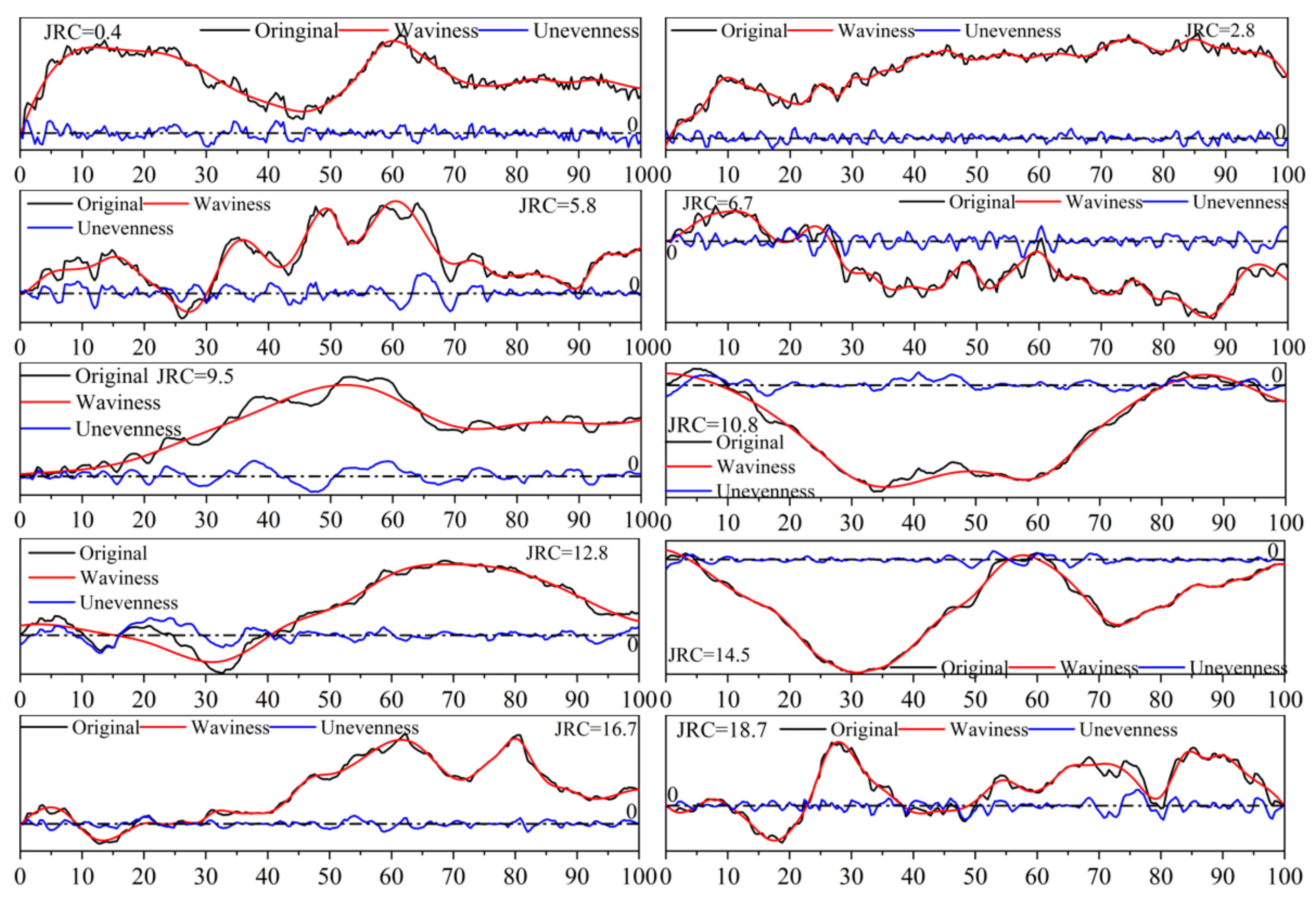
2.2.4. Decomposition Result of the Standard JRC Profile

The ten standard JRC profiles were decomposed by the method combining the EEMD and the critical decomposition level criterion. The decomposition results are shown in Figure 6.

The waviness component met the characteristics of large amplitude and low frequency, which basically reflected the macroscopic fluctuation characteristics of the standard JRC profile. The unevenness component satisfied the characteristics of small amplitude (fluctuation around 0, basically) and high frequency, as shown in Figure 6. The characteristics of the waviness and unevenness satisfied the definition of the ISRM.

3. The Mechanical Contribution of Waviness and Unevenness

3.1. Shear Test

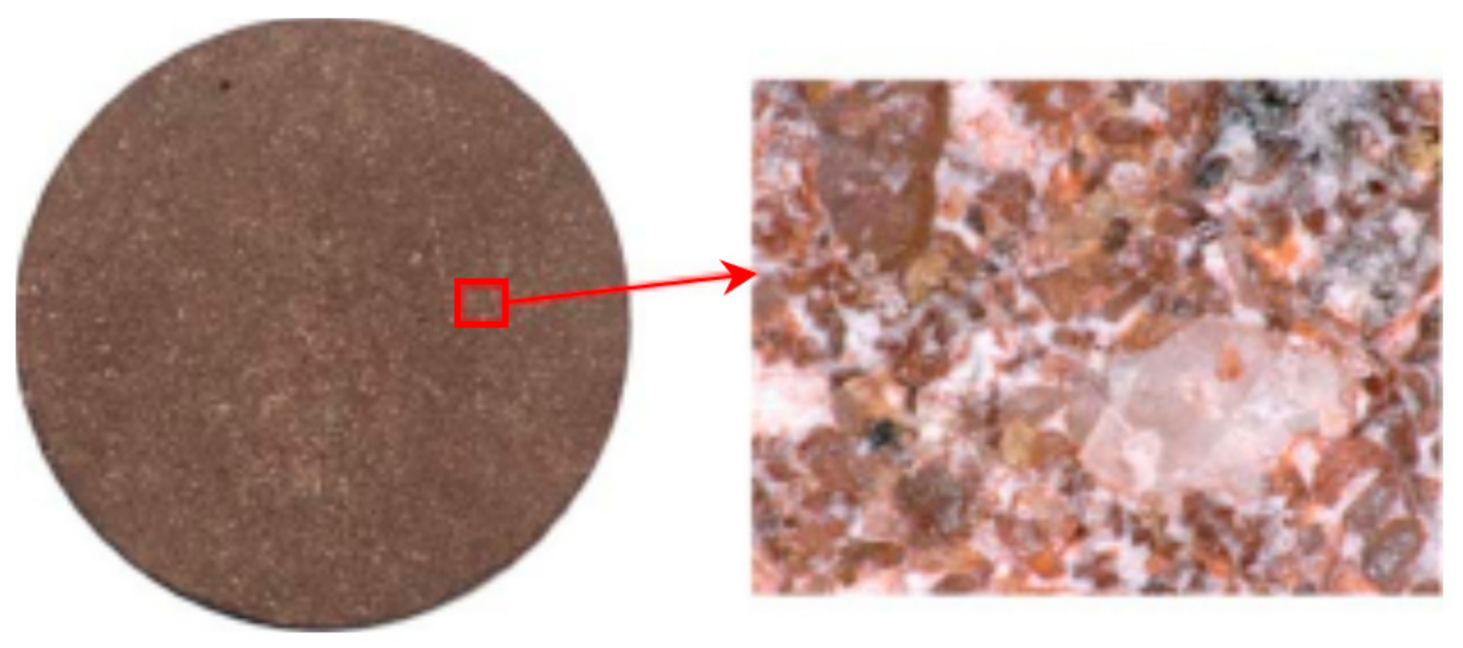
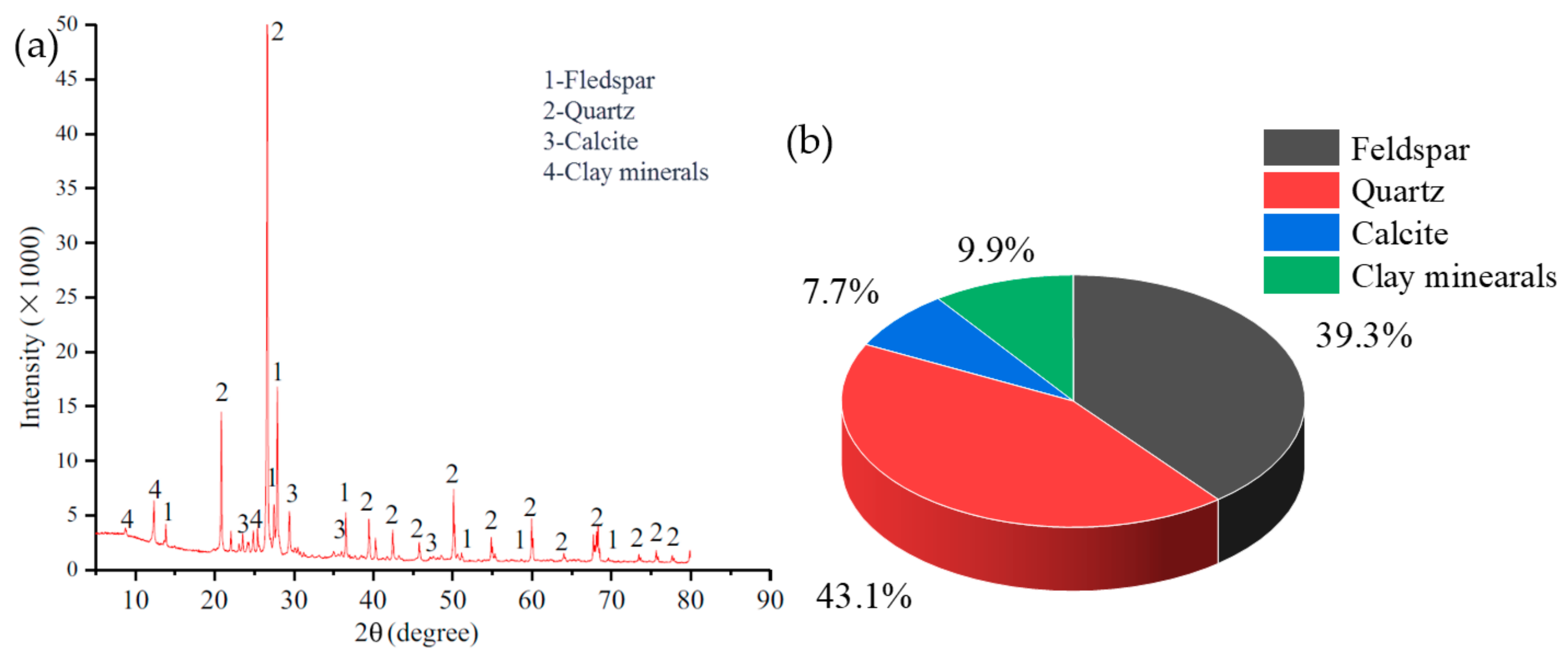
3.1.1. Joint Specimen Preparation and Test Schemes

As no two natural rock joint specimens are truly identical, it is difficult to obtain a large number of specimens with the same morphology [74]. Therefore, when testing schemes require multiple specimens, joint specimens with natural surfaces are produced mainly by copying techniques, such as creating fractures by splitting, sawing flat joints with undulated or irregular surfaces, and casting natural or stylized joints with silicon or rubber molds. However, the mechanical properties of casting material [75] are different from rock material. Thus, it is difficult to reflect the mechanical properties and failure mechanisms of joint specimens. Three-dimensional engraving technology [76] can produce a large number of joint specimens with the same morphology using rock as the raw material, thus avoiding the use of casting materials and rock materials that have different mechanical properties. In this study, a 3D engraving machine (MK-6060) was used to prepare joint specimens. The engraving system is composed of a control system, spindle, operating floor, cooling water circulation system, and milling cutter, as shown in Figure 7. The control system is used to control the movement of the spindle. The precision is 0.1 mm, which meets the accuracy requirement. The raw material used in the test was red sandstone, which was collected from Dawu County, Hubei province, China. It is a medium coarse quartz sandstone with an average grain size of 0.25~0.5 mm. The mineral composition of this red sandstone was identified by XRD test (Figure 8), showing the main mineral composition to include feldspar (39.25%), quartz (43.14%), calcite (7.7%), kaolinite (3.17%), illite (1.98%), chlorite (3.76%), and mixed-layer illite/montomrillonite (0.1%). Figure 9 shows the structure of the red sandstone. The mechanical properties of the red sandstone were tested by compression and shear tests, as listed in

Table 3. Basic mechanical properties of red sandstone.

Uniaxial Compressive Strength (UCS) /MPa	Cohesion Stress /MPa	Friction Angle /°	E /GPa
48	7.03	47.23	16.27

.

The engraving consisted of four basic steps, as follows:

• Importing the digitization data into CAD software to generate the profile;
• Stretching the profile onto the surface using the stretch command in CAD software and exporting the surface in .igs format;
• Importing the surface file into JD-Paint software and generating an engraving path file;
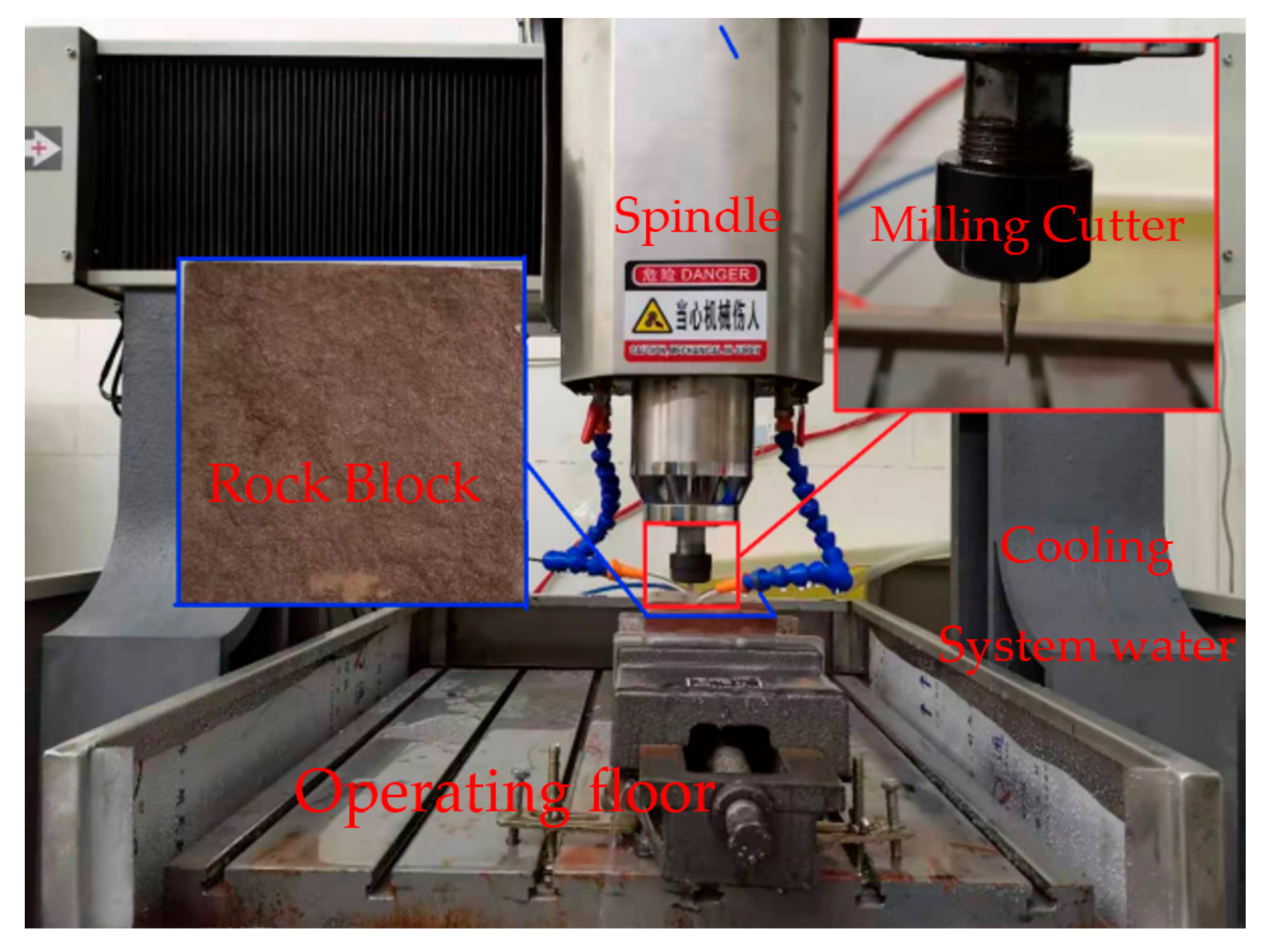
• Fixing the standard sandstone on the operating floor, then turning on the engraving machine.

In order to analyze the mechanical contribution of waviness and unevenness to the shear strength of the joint specimen, three kinds of joint specimens were prepared (the Standard JRC profiles 5^#~10^#, the profile containing only waviness, and the profile with the flat surface). A total of 39 groups of joint specimens were prepared. Three normal stresses were applied in this shear test, and the test schemes are shown in

Table 4. Shear test schemes.

Joint Roughness Coefficient	Asperity Order	Normal Stress
Flat (0)		0.6 MPa, 2.4 MPa, 4.8 MPa (0.0125UCS, 0.05UCS, 0.1UCS)
JRC = 9.5	Waviness + Unevenness	0.6 MPa, 2.4 MPa, 4.8 MPa
	Waviness	0.6 MPa, 2.4 MPa, 4.8 MPa
JRC = 10.8	Waviness + Unevenness	0.6 MPa, 2.4 MPa, 4.8 MPa
	Waviness	0.6 MPa, 2.4 MPa, 4.8 MPa
JRC = 12.8	Waviness + Unevenness	0.6 MPa, 2.4 MPa, 4.8 MPa
	Waviness	0.6 MPa, 2.4 MPa, 4.8 MPa
JRC = 14.5	Waviness + Unevenness	0.6 MPa, 2.4 MPa, 4.8 MPa
	Waviness	0.6 MPa, 2.4 MPa, 4.8 MPa
JRC = 16.7	Waviness + Unevenness	0.6 MPa, 2.4 MPa, 4.8 MPa
	Waviness	0.6 MPa, 2.4 MPa, 4.8 MPa
JRC = 18.7	Waviness + Unevenness	0.6 MPa, 2.4 MPa, 4.8 MPa
	Waviness	0.6 MPa, 2.4 MPa, 4.8 MPa

.

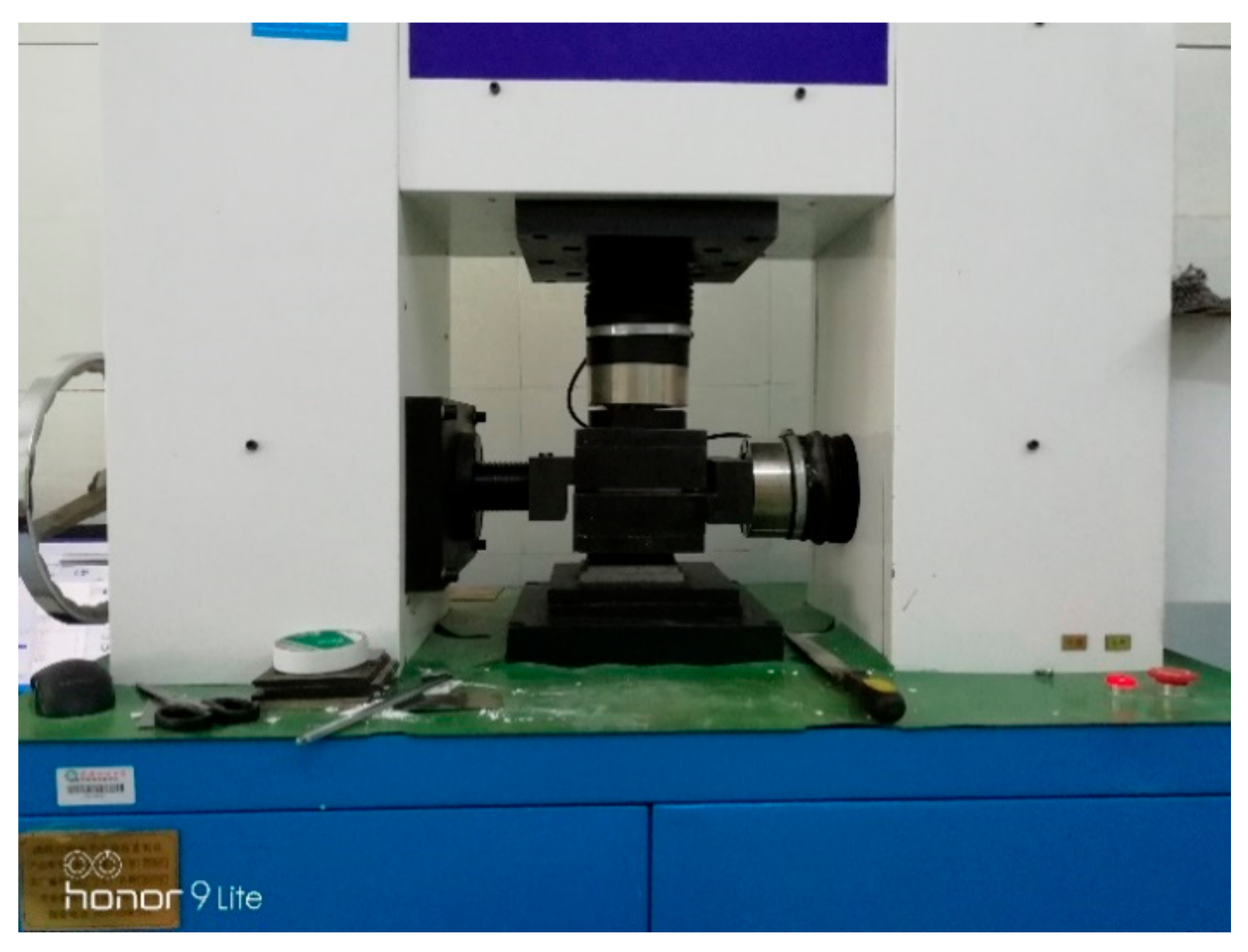
3.1.2. Test Equipment

The direct shear tests were performed with a YZW-30A rock mechanics test system, which is a computer-controlled electronic testing machine (Figure 10). Its maximum axial (tangential) load is 250 kN, and its loading methods include displacement control and stress control. The loading test was carried out in two steps: normal stress loading and shear stress loading. When the normal stress reached the target value, it was held, and the shear stress loading was started. When the shear displacement reached the target value, the test was stopped. The loading mode of normal stress and shear stress was the displacement control mode. The loading process was evenly divided into two steps. First, the loading was carried out at a higher loading rate (0.6 mm/min) to realize the rapid contact between the pressure head and the surface of the shear box. When the stress reached the initial target value (0.2 kN), the loading rate decreased to 0.3 mm/min (ISRM 2014 [77]). The maximum shear displacement of the loading system was 10 mm. In order to prevent damage to the test equipment caused by excessive shear displacement, the shear test automatically stopped when the shear displacement reached 8 mm.

3.2. Contribution of Waviness and Unevenness to the Shear Strength

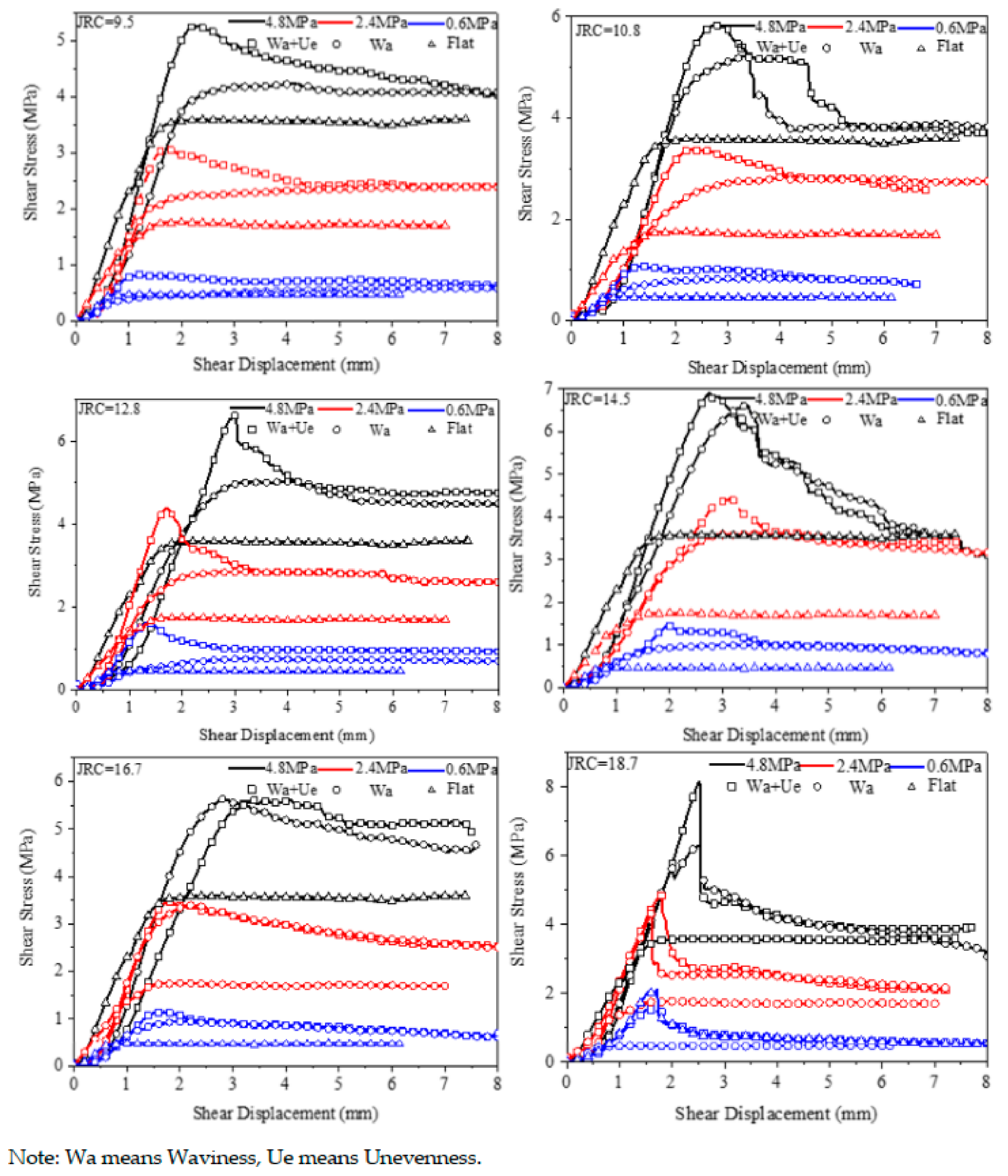
3.2.1. Shear Test Result

According to the test scheme, a series of shear tests were carried out with the red sandstone joint specimens, and the shear stress–shear displacement curves are shown in Figure 11.

The strength difference between the joint specimen that contained two-order asperity and the specimen whose surface was flat gradually increased with the normal stress increase. The strength difference between the joint specimen that contained two-order asperity and the joint specimen that contained only waviness gradually decreased with the normal stress increase, as shown in Figure 11.

3.2.2. Contribution of Waviness and Unevenness to the Shear Strength

In order to quantify the mechanical contribution of waviness and unevenness, the parameter $K_{asperity}$ was defined as a coefficient to represent the mechanical contribution of the asperities to the joint’s shear strength (Equation (5)).

$$K_{asperity}=\frac{{\tau }_{p\_Wa+Ue}-{\tau }_{p\_Flat}}{{\tau }_{p\_Wa+Ue}}$$

(5)

where ${\tau }_{p\_Wa+Ue}$ and ${\tau }_{p\_Flat}$ are equal to the shear strengths of the joint specimen with two-order asperity and the specimen with the flat surface, respectively.

The values of $K_{asperity}$ under different normal stresses with different roughness were calculated and are plotted in Figure 12. The parameter $K_{asperity}$ values gradually decreased with increasing normal stress (as shown in Figure 12), which indicated that the mechanical contribution of asperity to the joint specimen’s strength decreased with the normal stress increase. Under the normal stress, the parameter $K_{asperity}$ increased with the roughness increase. The above results showed that there was a relationship between the contribution degree $K_{asperity}$ and the roughness coefficient of the joint surface.

In order to further investigate the contribution of waviness and unevenness to the joint’s shear strength, $K_{asperity\_Wa}$ and $K_{asperity\_Ue}$ were defined as coefficients representing the mechanical contribution of waviness and unevenness to the joint’s shear strength (Equations (7) and (8)), respectively.

$${\tau }_{p\_Ue}={\tau }_{p\_Wa+Ue}-{\tau }_{p\_Wa}$$

(6)

$$K_{asperity\_Wa}=\frac{{\tau }_{p\_Wa}-{\tau }_{p\_Flat}}{{\tau }_{p\_Wa+Ue}-{\tau }_{p\_Flat}}\times K_{asperity}$$

(7)

$$K_{asperity\_Ue}=\frac{{\tau }_{p\_Ue}-{\tau }_{p\_Flat}}{{\tau }_{p\_Wa+Ue}-{\tau }_{p\_Flat}}\times K_{asperity}$$

(8)

where ${\tau }_{p\_Ue}$ equals the shear strength of the joint specimen containing only waviness.

The values of $K_{asperity\_Wa}$ and $K_{asperity\_Ue}$ under different normal stresses with different roughness were calculated and are shown in Figure 13a,b, respectively. The values of $K_{asperity\_Wa}$ and $K_{asperity\_Ue}$ decreased with the increase in normal stress. The values of $K_{asperity\_Wa}$ and $K_{asperity\_Ue}$ increased with the increase in joint roughness, as shown in Figure 13a,b. This result was different from Hong’s research [64], which showed that the mechanical contribution of the unevenness was independent of the statistical parameters of the unevenness. Thus, it was necessary to carry out further research on the correlation between the mechanical contribution and the statistical parameter.

4. Characterization of the Joint Surface Roughness Coefficient

4.1. Relationship between the Mechanical Contribution and Statistical Parameter

4.1.1. Statistical Parameters of Waviness and Unevenness

In order to study the relationship between the asperity’s mechanical contribution and its statistical parameters, the parameters Z₂ and R_P-1 of the standard JRC profile and the waviness component (1st order) and unevenness component (2nd order) were calculated, and the results are shown in Figure 14.

The statistical parameters (Z₂ and R_p-1) increased with the increase in roughness (as shown in Figure 14). There were some profile’s statistical parameters that did not obey this law, however. As shown in Figure 14a, the statistical parameter $Z_2^{2\mathrm{nd}}$ showed a decreasing trend from profile 4^# to 5^#, while the statistical parameter $Z_2^{1\mathrm{st}}$ showed an increasing trend at this position; the statistical parameter $Z_2^{2\mathrm{nd}}$ showed an increasing trend from profile 8^# to 9^#, while the statistical parameter showed a decreasing trend at this position (as shown in Figure 14a). According to the analysis, compared with the 5^# profile, the 4^# profile contained more unevenness and less waviness. Compared with the 9^# profile, the 8^# profile contained more unevenness and waviness. Gao [52] also found this trend.

In order to analyze the mechanical contribution difference between the waviness component and the unevenness component, $K_{W-U}$ was defined as the parameter representing the mechanical contribution ratio of the waviness and the unevenness. The value of $K_{W-U}$ was calculated and is shown in Figure 15. $K_{W-U}$ barely changed with the normal stress increase.

In order to further establish the relationship between the mechanical contribution and the statistical parameters, the ratio of the statistical parameters of waviness to unevenness was calculated, and the calculated results are shown in Figure 16. Comparing Figure 15 and Figure 16, we found that the mechanical contribution ratio of the waviness and unevenness and the statistical parameter ratio of the waviness and unevenness showed an opposite trend. K_W-U and the statistical parameter ratio of the waviness and unevenness showed different change laws. The larger the K_W-U, the smaller the statistical parameter ratio of the waviness and unevenness. In Figure 15, K_W-U-9.5 > K_W-U-12.5 > K_W-U-10.8 > K_W-U-16.7 > K_W-U-18.7; at the same time, (Z₂^1st/Z₂^2nd)_9.5 < (Z₂^1st/Z₂^2nd)_12.5 < (Z₂^1st/Z₂^2nd)_10.8 < (Z₂^1st/Z₂^2nd)_16.7 < (Z₂^1st/Z₂^2nd)_18.7. Zhu [78] also found this trend in his research.

4.1.2. Relationship between the Mechanical Contribution and Statistical Parameter

In order to further explore the relationship between the mechanical contribution ratio and the statistical parameter ratio, the relationship between them was fitted; the fitting results are shown in Figure 17a,b. It can be seen in Figure 17 that there is a relationship between the mechanical contribution ratio and the statistical parameter ratio. This relation can be described by the power function.

4.2. Roughness Characterization Formula Considering the Mechanical Contribution

The mechanical contributions of different asperity orders are different. There is a relationship between the mechanical contribution and the statistical parameters. Therefore, it was necessary to establish a formula representing the joint roughness that accurately considered the mechanical contributions of different asperity orders. The shear strength can be divided into three parts [48]: the basic frictional resistance, the resistance provided by the waviness, and the resistance provided by the unevenness, as shown in Equation (9).

$$\tau ={\tau }_{Wa}+{\tau }_{Ue}+{\tau }_b$$

(9)

Hong [56] divided the joint surface into waviness and unevenness by different interval methods and established a formula representing the joint surface roughness, considering the statistical parameters of waviness and unevenness (Equation (10)).

$$JRC=\mathrm{a}\times {\left(P^{1\mathrm{st}}\right)}^m+b\times {\left(P^{2\mathrm{nd}}\right)}^n+c$$

(10)

Inserting Equations (11) and (12) into Barton’s formula, it is rewritten as Equation (11).

$${\tau }_p={\tau }_{p\_Wa+Ue}={\sigma }_n\tan \left[\left(a\times {(P^{1\mathrm{st}})}^m+b\times {\left(p^{2\mathrm{nd}}\right)}^n+c\right)·{\log }_{10}\left(\frac{JCS}{{\sigma }_n}\right)+{\varphi }_b\right]$$

(11)

By decomposing c in Equation (13) into two parts, c₁ and c₂, Equation (13) is rewritten as Equation (12).

$${\tau }_p={\tau }_{p\_Wa+Ue}={\sigma }_n\tan \left[\left(a\times {(P^{1\mathrm{st}})}^m+c_1+b\times {\left(p^{2\mathrm{nd}}\right)}^n+c_2\right)·{\log }_{10}\left(\frac{JCS}{{\sigma }_n}\right)+{\varphi }_b\right]$$

(12)

where $a\times {(P^{1\mathrm{st}})}^m+c_1$ represents the waviness’s roughness, and $b\times {\left(p^{2\mathrm{nd}}\right)}^n+c_2$ represents the unevenness’s roughness.

Therefore, Equation (14) is transformed into Equation (13).

$${\tau }_p={\tau }_{p\_Wa+Ue}={\sigma }_n\tan \left[\left(JR{C}^{1\mathrm{st}}+JR{C}^{2\mathrm{nd}}\right)·{\log }_{10}\left(\frac{JCS}{{\sigma }_n}\right)+{\varphi }_b\right]$$

(13)

For joint specimens that contain only waviness, the shear strength equation is expressed as Equation (14).

$${\tau }_p={\tau }_{p\_Wa}={\sigma }_n\tan \left[JR{C}^{1\mathrm{st}}·{\log }_{10}\left(\frac{JCS}{{\sigma }_n}\right)+{\varphi }_b\right]$$

(14)

In order to calculate JRC^1st and JRC^2nd, Equations (13) and (14) are deduced backward, and the results are shown in Equations (15) and (16).

$$JR{C}^{1\mathrm{st}}+JR{C}^{2\mathrm{nd}}=\left(\arctan \left(\frac{{\tau }_{p\_Wa+Ue}}{{\sigma }_n}\right)-{\varphi }_b\right)/{\log }_{10}\left(\frac{JCS}{{\sigma }_n}\right)$$

(15)

$$JR{C}^{1\mathrm{st}}=\left(\arctan \left(\frac{{\tau }_{p\_Wa}}{{\sigma }_n}\right)-{\varphi }_b\right)/{\log }_{10}\left(\frac{JCS}{{\sigma }_n}\right)=a\times {(P^{1\mathrm{st}})}^m+c_1$$

(16)

The second-order roughness coefficient JRC^2nd is obtained by subtracting Equation (16) from Equation (15), as shown in Equation (17).

$$JR{C}^{2\mathrm{nd}}=\left(\arctan \left(\frac{{\tau }_{p\_Wa+Ue}}{{\sigma }_n}\right)-\arctan \left(\frac{{\tau }_{p\_Wa}}{{\sigma }_n}\right)\right)/{\log }_{10}\left(\frac{JCS}{{\sigma }_n}\right)=b\times {\left(p^{2\mathrm{nd}}\right)}^n+c_2$$

(17)

Equations (16) and (17) are fitted according to the statistical parameters given in Figure 12; the fitting results are shown in Figure 18.

According to the fitting result, the formula considering the mechanical contribution of the waviness and unevenness was established, as shown in Equations (18) and (19).

$$JRC=379.6{\left(Z_2^{1\mathrm{st}}\right)}^{1.162}+3.223\times {10}^{-10}{\left(Z_2^{2\mathrm{nd}}\right)}^{-8.205}+0.596$$

(18)

$$JRC=4853{\left(R_P^{1\mathrm{st}}-1\right)}^{2.06}+9.427\times {10}^{-5}{\left(R_P^{2\mathrm{nd}}-1\right)}^{-2.475}+7.969$$

(19)

The correlation coefficients (R²) of the characterization formula based on the statistical parameters $Z_2^{1\mathrm{st}}$ and $Z_2^{1\mathrm{st}}$ are 0.8491 and 0.8531, respectively; The R² of the characterization formula based on the statistical parameters $R_P^{1\mathrm{st}}-1$ and $R_P^{2\mathrm{nd}}-1$ are 0.9504 and 0.9046, respectively. According to R², we can conclude that Equations (18) and (19) can be used to characterize joint roughness. Compared with the formula shown in Table 1, the formula proposed in this study (Equations (18) and (19)) considers the contribution of waviness and unevenness. Compared with the formula shown in Table 2, the formula proposed in this study not only considers the morphology contribution of each asperity order, but also considers the mechanical contribution of each asperity order.

5. Conclusions

In order to establish a formula that characterizes joint roughness, considering the mechanical contribution of each asperity order, shear tests were carried out on 39 groups of red sandstone joint specimens with seven different roughness degrees (5^#~10^# standard JRC profile and flat) and two asperity orders under three different normal stresses. The mechanical contribution of each asperity order was analyzed, and the relationship between the mechanical contribution of each asperity order and its statistical parameters was explored. The conclusions are as follows:

(1)

A new decomposition method of joint surface roughness is proposed. The ensemble empirical mode decomposition (EEMD) in this method does not require an a priori basis function, and the critical decomposition level criterion in this method has a clear mathematical definition. The standard JRC profile can be decomposed into waviness and unevenness by the method combining the EEMD and the critical decomposition level.

(2)

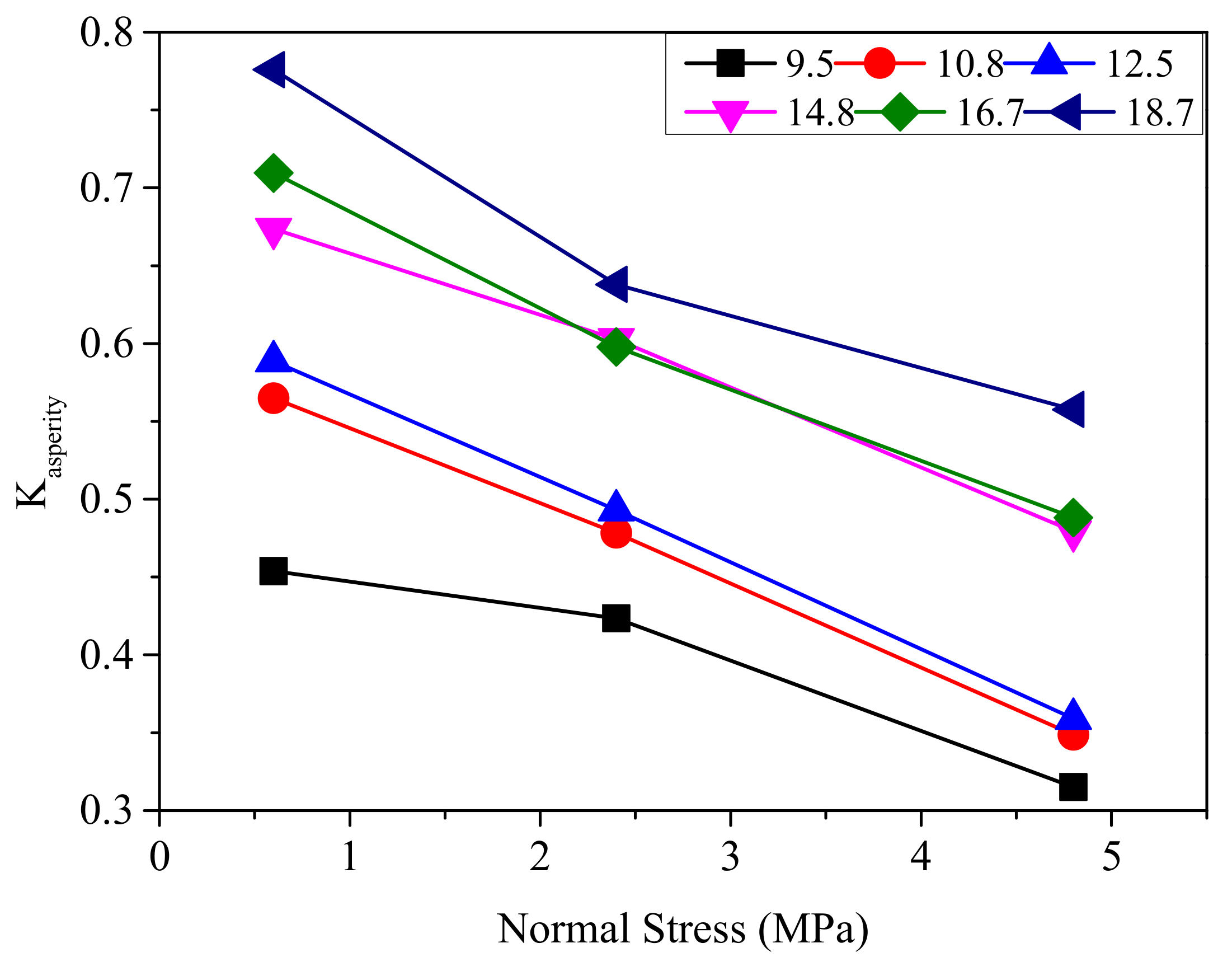
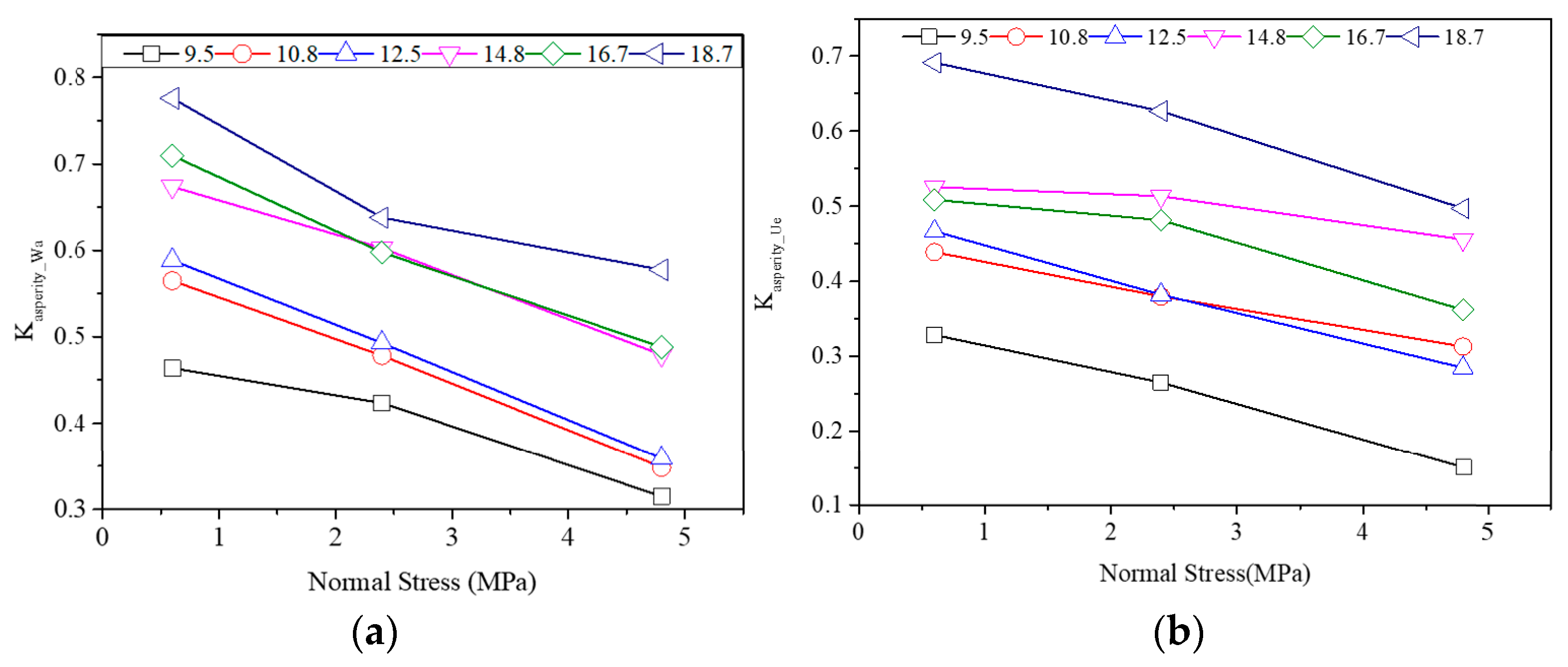
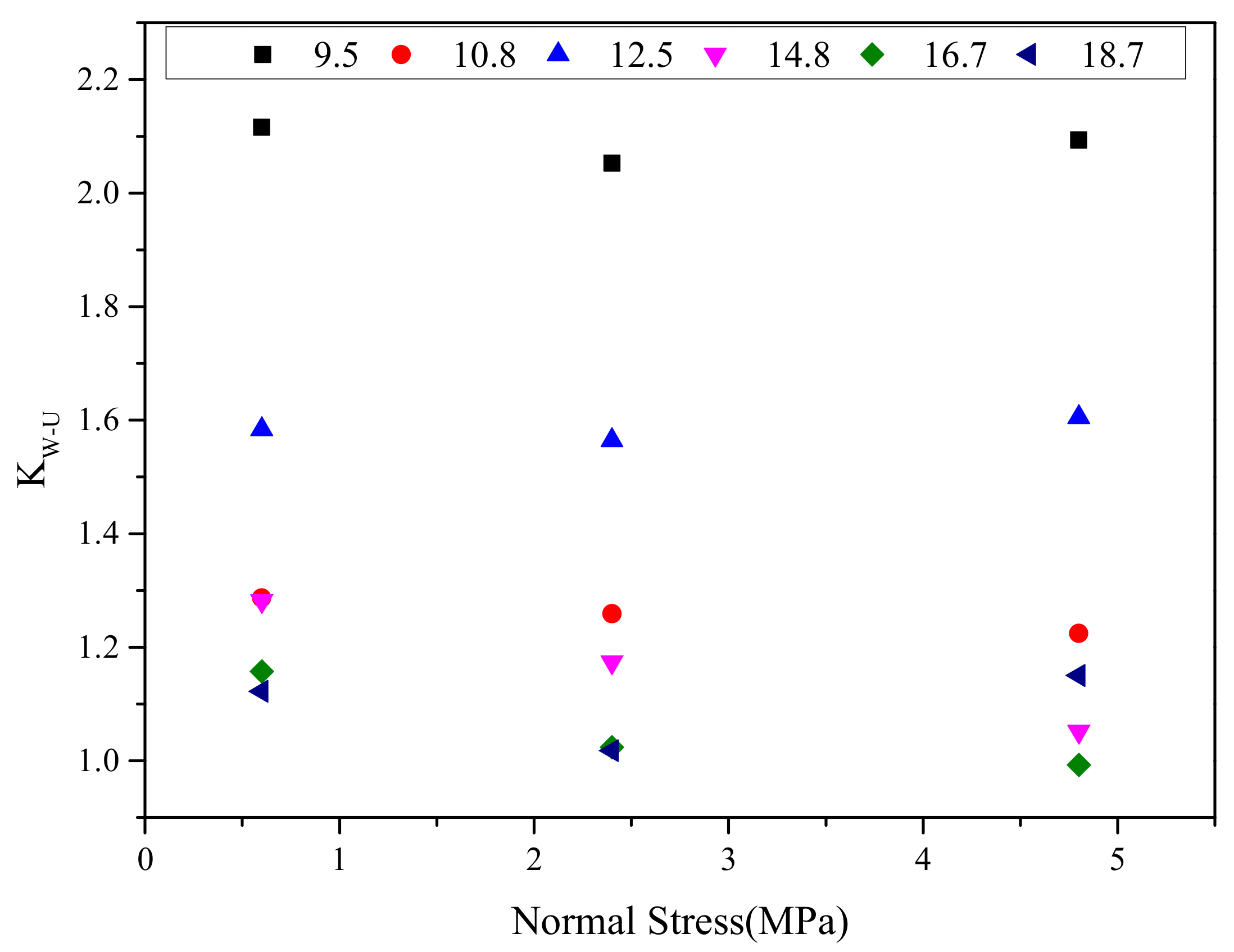
The mechanical contribution of waviness and unevenness is related to normal stress. The ratio between them is less affected by normal stress. The mechanical contribution of the waviness and the unevenness decreases with the increase in normal stress, which means that as normal stress increases, the influence of the joint surface morphology on the shear strength gradually decreases. At the same time, the mechanical contribution ratio of waviness and unevenness hardly changes with the change in normal stress.

(3)

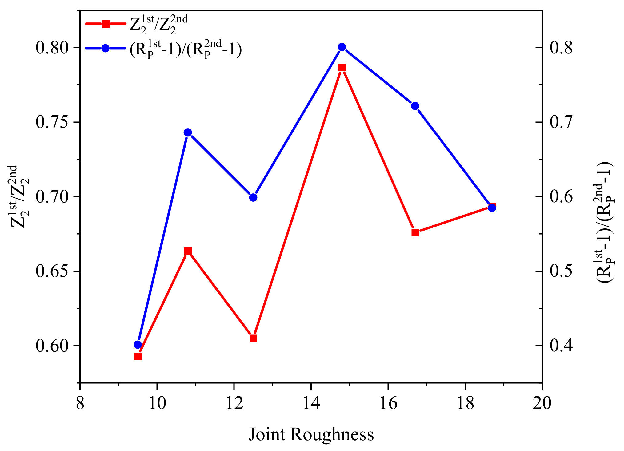
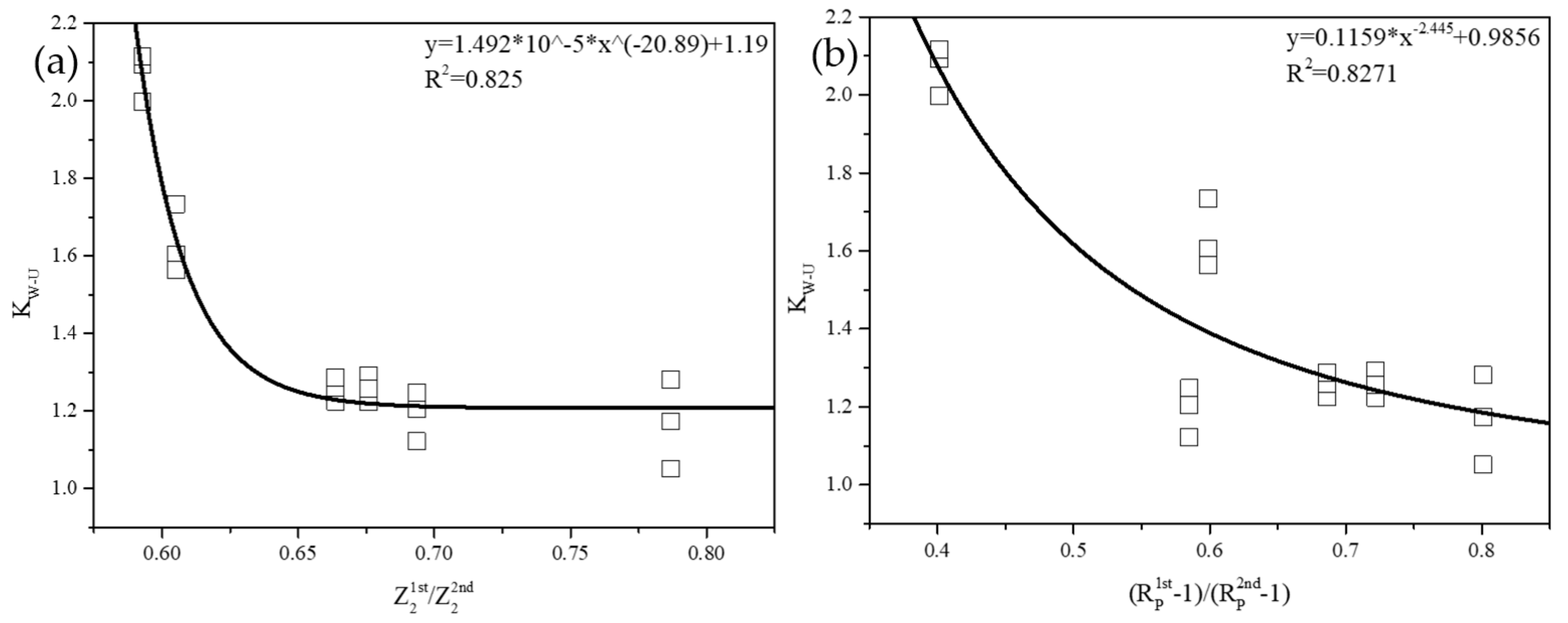
The mechanical contribution of waviness and unevenness is related to their statistical parameter contribution. The relationship between the mechanical contribution ratio of waviness and unevenness and its statistical parameter ratio can be describe by the power function. The mechanical contribution ratio of waviness and unevenness decreases with the increase in their statistical parameter ratio, which means that it is difficult to accurately characterize the roughness of the joint surface by considering only the contribution of the statistical parameter. In order to characterize the roughness of the joint surface accurately, we should consider not only the contribution of the statistical parameter, but also the mechanical contribution.

(4)

A formula for characterizing the roughness of the joint surface is established that considers the morphology contribution of waviness and unevenness and their mechanical contributions at the same time. Compared with the formula that only considers the statistical parameters of the joint surface, this formula fully considers the mechanical contribution of each asperity order. This formula is of great significance for accurately characterizing the roughness of the joint surface and evaluating the shear strength of the joint.

References

1. Hoek, E. Shear Strength of Discontinuities. In Practical Rock Engineering; Evert Hoek Consulting Engineer Inc.: North Vancouver, BC, Canada, 2007; pp. 1–14. [Google Scholar]
2. Mineo, S.; Pappalardo, G.; Onorato, S. Geomechanical characterization of a rock cliff hosting a cultural heritage through ground and UAV rock mass surveys for its sustainable fruition. Sustainability 2021, 13, 924. [Google Scholar] [CrossRef]
3. Pappalardo, G.; Mineo, S.; Imposa, S.; Grassi, S.; Leotta, A.; La Rosa, F.; Salerno, D. A quick combined approach for the charac-terization of a cliff during a post-rockfall emergency. Landslides 2020, 17, 1063–1081. [Google Scholar] [CrossRef]
4. Mineo, S.; Pappalardo, G. Sustainable fruition of cultural heritage in areas affected by rockfalls. Sustainability 2019, 12, 296. [Google Scholar] [CrossRef] [Green Version]
5. Mineo, S.; Pappalardo, G. Study of jointed and weathered rock slopes through the innovative approach of InfraRed thermography. In Advances in Natural and Technological Hazards Research, Landslides: Theory, Practice and Modelling; Pradhan, S.P., Vishal, V., Singh, T.N., Eds.; Springer: Berlin, Germany, 2019; pp. 85–103. [Google Scholar]
6. Pappalardo, G.; Imposa, S.; Mineo, S.; Grassi, S. Evaluation of the stability of a rock cliff by means of geophysical and geomechanical surveys in a cultural heritage site (south-eastern Sicily). Ital. J. Geosci. 2016, 135, 308–323. [Google Scholar] [CrossRef]
7. An, P.J.; Fang, K.; Jiang, Q.Q.; Zhang, H.H.; Zhang, Y. Measurement of rock joint surfaces by using smartphone structure from motion (SfM) photogrammetry. Sensors 2021, 21, 922. [Google Scholar] [CrossRef]
8. Rasouli, V.; Harrison, J.P. Assessment of rock fracture surface roughness using Riemannian statistics of linear profiles. Int. J. Rock Mech. Min. Sci. 2010, 47, 940–948. [Google Scholar] [CrossRef]
9. Ban, L.R.; Du, W.S.; Qi, C.Z.; Zhu, C. Modified 2D roughness parameters for rock joints at two different scales and their correlation with JRC. Int. J. Rock Mech. Min. Sci. 2021, 137, 104549. [Google Scholar] [CrossRef]
10. Wong, L.N.Y.; Meng, F.Z.; Zhou, H.; Yu, J.; Cheng, G.T. Influence of the choice of reference planes on the determination of 2D and 3D joint roughness parameters. Rock Mech. Rock Eng. 2021, 1–14. [Google Scholar] [CrossRef]
11. Bao, H.; Xu, X.H.; Lan, H.X.; Zhang, G.B.; Yin, P.J.; Yan, C.G.; Xu, J.B. A new joint morphology parameter considering the effects of micro-slope distribution of joint surface. Eng. Geol. 2020, 275, 105734. [Google Scholar] [CrossRef]
12. Barton, N. Review of a new shear-strength criterion for rock joints. Eng. Geol. 1973, 7, 287–332. [Google Scholar] [CrossRef]
13. Barton, N.; Choubey, V. The shear strength of rock joints in theory and practice. Rock Mech. 1977, 10, 1–54. [Google Scholar] [CrossRef]
14. ISRM. International socieity for rock mechanics commision on standardization of laboratory and field tests: Suggested methods for the quantitative description of discontinuities in rock masses. Int. J. Rock Mech. Min. Sci. Geomech. Abstr. 1978, 15, 319–368. [Google Scholar] [CrossRef]
15. Beer, A.J.; Stead, D.; Coggan, J.S. Technical note estimation of the joint roughness coefficient (JRC) by visual comparison. Rock Mech. Rock Eng. 2002, 35, 65–74. [Google Scholar] [CrossRef]
16. Alameda-Hernandez, P.; Jimenez-Peralvarez, J.; Palenzuela, J.A.; Hamdouni, R.I.; Iri-garay, I.; Cabrerizo, M.A.; Chacon, J. Improvement of the JRC calculation using different parameters obtained through a new survey method applied to rock discontinuities. Rock Mech. Rock Eng. 2014, 47, 2047–2060. [Google Scholar] [CrossRef]
17. García-Luna, R.; Senent, S.; Jimenez, R. Characterization of joint roughness using long-range terrestrial photogrammetry. In Proceedings of the ISRM International Symposium—EUROCK 2020, Trondheim, Norway, 14 June 2020. [Google Scholar]
18. Tse, R.; Cruden, D.M. Estimating joint roughness coefficients. Int. J. Rock Mech. Min. Sci. Geomech. Abst. 1979, 16, 303–307. [Google Scholar] [CrossRef]
19. Magsipoc, E.; Zhao, Q.; Grasselli, G. 2D and 3D roughness characterization. Rock Mech. Rock Eng. 2020, 53, 1495–1519. [Google Scholar] [CrossRef]
20. Yu, X.B.; Vayssade, B. Joint profiles and their roughness parameters. Int. J. Rock Mech. Min. Sci. Geomech. Abstr. 1991, 28, 333–336. [Google Scholar] [CrossRef]
21. Yang, Z.Y.; Lo, S.C.; Di, C.C. Reassessing the joint roughness coefficient (JRC) estimation using Z2. Rock Mech. Rock Eng. 2001, 34, 243–251. [Google Scholar] [CrossRef]
22. Tatone, B.S.A.; Grasselli, G. A new 2D discontinuity roughness parameter and its correlation with JRC. Int. J. Rock Mech. Min. Sci. 2010, 47, 1391–1400. [Google Scholar] [CrossRef]
23. Jang, H.S.; Kang, S.S.; Jang, B.A. Determination of joint roughness coefficients using roughness parameters. Rock Mech. Rock Eng. 2014, 47, 2061–2073. [Google Scholar] [CrossRef]
24. Li, Y.R.; Zhang, Y.B. Quantitative estimation of joint roughness coefficient using statistical parameters. Int. J. Rock Mech. Min. Sci. 2015, 77, 27–35. [Google Scholar] [CrossRef] [Green Version]
25. Abolfazli, M.; Fahimifar, A. An investigation on the correlation between the joint rough-ness coefficient (JRC) and joint roughness parameters. Constr. Build. Mater. 2020, 259, 120415. [Google Scholar] [CrossRef]
26. Sun, F.T.; She, C.X.; Wan, L.T. Research on relationship between JRC of Barton’s standard profiles and statistic parameters independent of sampling intrval. Chin. J. Rock Mech. Eng. 2014, 33, 2513–2519. (In Chinese) [Google Scholar]
27. Maerz, N.H.; Franklin, J.A.; Bennett, C.P. Joint roughness measurement using shadow profilometry. Int. J. Rock Mech. Min. Sci. Geomech. Abstr. 1990, 27, 329–343. [Google Scholar] [CrossRef]
28. Zheng, B.W.; Qi, S.W. A new index to describe joint roughness coefficient (JRC) under cyclic shear. Eng. Geol. 2016, 212, 72–85. [Google Scholar] [CrossRef]
29. Belem, T.; Homand-Etienne, F.; Souley, M. Quantitative parameters for rock joint surface roughness. Rock Mech. Rock Eng. 2000, 33, 217–242. [Google Scholar] [CrossRef]
30. Zhang, Z.Q.; Huan, J.Y.; Li, N.; He, M.M. Suggested new statistical parameter for estimating joint roughness coefficient considering the shear direction. Adv. Civ. Eng. 2021, 2021, 8872873. [Google Scholar]
31. Zhang, G.C.; Karakus, M.; Tang, H.M.; Ge, Y.F.; Zhang, L. A new method estimating the 2D joint roughness coefficient for discontinuity surfaces in rock masses. Int. J. Rock Mech. Min. Sci. 2014, 72, 191–198. [Google Scholar] [CrossRef]
32. Grasselli, G.; Wirth, J.; Egger, P. Quantitative three-dimensional description of a rough surface and parameter evolution with shearing. Int. J. Rock Mech. Min. 2002, 39, 789–800. [Google Scholar] [CrossRef]
33. Zhang, Z.Q.; Huan, J.Y.; He, M.M.; Li, N. A New Statistical Parameter for Determining Joint Roughness Coefficient (JRC) considering the Shear Direction and Contribution of Different Protrusions. Adv. Civ. Eng. 2021, 2021, 6641201. [Google Scholar]
34. Liu, Q.S.; Tian, Y.C.; Liu, D.F.; Jiang, Y.L. Updates to JRC-JCS model for estimating the peak shear strength of rock joints based on quantified surface description. Eng. Geol. 2017, 228, 282–300. [Google Scholar] [CrossRef]
35. Chen, X.; Zeng, Y.W.; Ye, Y.; Sun, H.Q.; Tang, Z.C.; Zhang, X.B. A Simplified form of Grasselli′s 3D roughness measure θ max */(C + 1). Rock Mech. Rock Eng. 2021, 1–18. [Google Scholar] [CrossRef]
36. Develi, K. Computation of direction dependent joint surface parameters through the algo-rithm of triangular prism surface area method: A theoretical and experimental study. Int. J. Solids Struct. 2020, 202, 895–911. [Google Scholar] [CrossRef]
37. Pickering, C.; Aydin, A. Modeling roughness of rock discontinuity surfaces: A signal analysis approach. Rock Mech. Rock Eng. 2016, 49, 2959–2965. [Google Scholar] [CrossRef]
38. Ünlüsoy, D.; Süzen, M.L. A new method for automated estimation of joint roughness coefficient for 2D surface profiles using power spectral density. Int. J. Rock Mech. Min. Sci. 2020, 125, 104156. [Google Scholar] [CrossRef]
39. Kou, M.M.; Liu, X.R.; Tang, S.D.; Wang, Y.T. Experimental study of the prepeak cyclic shear mechanical behaviors of artificial rock joints with multiscale asperities. Soil Dyn. Earthq. Eng. 2019, 120, 58–74. [Google Scholar] [CrossRef]
40. Nigon, B.; Englert, A.; Pascal, C.; Santot, A. Multiscale characterization of joint surface roughness. J. Geophy. Res-Sol Ea. 2017, 122, 9714–9728. [Google Scholar] [CrossRef]
41. Liu, X.R.; Xu, B.; Lin, G.; Huang, J.; Zhou, X.; Xie, Y.; Wang, J.; Xiong, F. Experimental and numerical investigations on the macro-meso shear mechanical behaviors of artificial rock discontinuities with multiscale asperities. Rock Mech. Rock Eng. 2021, 1–20. [Google Scholar] [CrossRef]
42. Li, Y.C.; Wu, W.; Wei, X. Analytical modeling of the shear behavior of rock joints with two-order asperity dilation and degradation. Int. J. Geomech. 2020, 20, 04020062. [Google Scholar] [CrossRef]
43. Lee, S.W. Stability around Underground Openings in Rock with Dilative, Non-Persistent and Multi-Scale Wavy Joints Using a Discrete Element Method; University of Illinois at Urbana-Champaign: Champaign, IL, USA, 2003. [Google Scholar]
44. Jing, L.R.; Stephansson, O.S.; Nordlund, E. Study of rock joints under cyclic loading con-ditions. Rock Mech. Rock Eng. 1993, 26, 215–232. [Google Scholar] [CrossRef]
45. Plesha, M. Constitutive models for rock discontinuities and surface degradation. Int. J. Numer. Anal Methods Geomech. 1987, 11, 345–362. [Google Scholar] [CrossRef]
46. Kana, D.D.; Fox, D.J.; Hsiung, S.M. Interlock/friction model for dynamic shear response in natural jointed rock. Int. J. Rock Mech. Min. Sci. Geomech. Abstr. 1996, 33, 371–386. [Google Scholar] [CrossRef]
47. Li, Y.C.; Sun, S.Y. Analytical prediction of the shear behaviour of rock joints with quanti-fied waviness and unevenness through wavelet analysis. Rock Mech. Rock Eng. 2019, 52, 3645–3657. [Google Scholar] [CrossRef]
48. Hong, E.S.; Lee, J.S.; Lee, I.M. Underestimation of roughness in rock joints. Int. J. Numer. Anal Methods Geomech. 2008, 32, 1385–1403. [Google Scholar] [CrossRef]
49. Chen, S.J.; Zhao, Z.H.; Wang, C. Estimation of rock joint roughness based on modified line-roughness. Met. Mine 2012, 41, 22–25. (In Chinese) [Google Scholar]
50. Chen, S.J.; Zhu, W.C.; Zhan, M.S.; Yu, Q.L. Fractal description of rock joints based on digital image processing technique. Chin. J. Geotech. Eng. 2012, 34, 2087–2092. (In Chinese) [Google Scholar]
51. Li, H.; Huang, R.Q. Method of quantitative determination of joint roughness coefficient. Chin. J. Rock Mech. Eng. 2014, 33, 3489–3497. (In Chinese) [Google Scholar]
52. Gao, Y.N.; Wong, L.N.Y. A modified correlation between roughness parameter Z2 and the JRC. Rock Mech. Rock Eng. 2015, 48, 387–396. [Google Scholar] [CrossRef]
53. Li, R.; Xiao, W.M. Study on a new equation for calculating JRC based on fine digization of standard profiles proposed by Barton. Chin. J. Rock Mech. Eng. 2018, 37, 3515–3523. (In Chinese) [Google Scholar]
54. Liu, X.G.; Zhu, W.C.; Yu, Q.L.; Chen, S.J.; Li, R.F. Estimation of the joint roughness coefficient of rock joints by consideration of two-order asperity and its application in double-joint shear tests. Eng. Geol. 2017, 220, 243–255. [Google Scholar] [CrossRef] [Green Version]
55. Liu, X.G.; Zhu, W.C.; Liu, Y.X.; Yu, Q.L.; Guan, K. Characterization of rock joint roughness from the classified and weigthed uphill projection parameters. Int. J. Geomech. 2021, 21, 04021052. [Google Scholar] [CrossRef]
56. Yang, Z.Y.; Taghichian, A.; Li, W.C. Effect of asperity order on the shear response of three-dimensional joints by focusing on damage area. Int. J. Rock Mech. Min. 2010, 47, 1012–1026. [Google Scholar] [CrossRef]
57. Xia, C.C.; Yue, Z.Q.; Tham, L.G.; Lee, C.F.; Sun, Z.Q. Quantifying topography and closure deformation of rock joints under normal stress. Int. J. Rock Mech. Min. 2003, 40, 197–220. [Google Scholar] [CrossRef]
58. Tang, Z.C.; Xia, C.C.; Jiao, Y.Y.; Wong, L.N.Y. Closure model with asperity interaction in normal contact for rock joint. Int. J. Rock Mech. Min. 2016, 100, 170–173. [Google Scholar] [CrossRef]
59. Jiang, Z.; Cao, P.; Fan, X.; He, Y.; Fan, W.C. Evolution of joint morphology subjected to shear loads based on Gaussion filtering method. J. Cent. South Univ. 2014, 45, 1975–1982. [Google Scholar]
60. Nie, Z.H.; Wang, X.; Huang, D.L.; Zhao, L.H. Fourier-shape-based reconstruction of rock joint profile with realistic unevenness and waviness features. J. Cent. South Univ. 2019, 26, 3103–3113. [Google Scholar] [CrossRef]
61. Ficker, T.; Dalibor, M. Alternative method for assessing the roughness coefficients of rock joints. J. Comput. Civ. Eng. 2016, 30, 04015059. [Google Scholar] [CrossRef]
62. Yong, R.; Ye, J.; Li, B.; Du, S.G. Determining the maximum sampling interval in rock joint roughness measurements using Fourier series. Int. J. Rock Mech. Min. 2018, 101, 78–88. [Google Scholar] [CrossRef]
63. Huang, M.; Hong, C.J.; Du, S.G.; Luo, Z.Y.; Zhang, G.Z. Study on morphological classification method and two-order roughness of rock joints. Chin. J. Rock Mech. Eng. 2020, 39, 1153–1164. [Google Scholar]
64. Hong, E.S.; Lee, I.M.; Cho, G.C.; Lee, S.W. New approach to quantifying rock joint roughness based on roughness mobilization characteristics. KSCE J. Civ. Eng. 2014, 18, 984–991. [Google Scholar] [CrossRef]
65. Zou, L.C.; Jing, L.R.; Cvetkovic, V. Roughness decomposition and nonlinear fluid flow in a single rock fracture. Int. J. Rock Mech. Min. 2015, 75, 102–118. [Google Scholar] [CrossRef]
66. Yang, Y.F.; Wu, Y.F. Common time-frequency analysis methods and their limitations. In Applications of Empirical Mode Decomposition in Vibration Analysis; Yang, Y.F., Wu, Y.F., Eds.; National Defense Industry Press: Beijing, China, 2013. [Google Scholar]
67. Gao, R.X.; Yan, R. From Fourier Transform to Wavelet Transform: A Historical Perspective; Springer US: Boston, MA, USA, 2011. [Google Scholar]
68. Duan, H.M.; Xie, F.; Zhang, K.; Ma, Y.; Shi, F. Signal trend extraction of road surface profile measurement. In Proceedings of the IEEE 2010 2nd International Conference on Signal Processing Systems (ICSPS), Dalian, China, 23 August 2010; pp. 694–698. [Google Scholar]
69. Huang, N.E.; Shen, Z.; Long, S.R.; Wu, M.L.; Shih, H.H.; Zheng, Q.; Yen, N.C.; Tung, C.C.; Liu, H.H. The empirical mode decomposition and the Hilbert spectrum for nonlinear and non-stationary time series analysis. Proc. R. Soc. Lond. Ser. A 1998, 454, 903–995. [Google Scholar] [CrossRef]
70. Li, B.; Wang, E.Y.; Shang, Z.; Li, Z.H.; Li, B.L.; Liu, X.F.; Wang, H.; Niu, Y.; Wu, Q.; Song, Y. Deep learning approach to coal and gas outburst recognition employing modified AE and EMR signal from empirical mode decomposition and time-frequency analysis. J. Nat. Gas. Sci. Eng. 2021, 90, 103942. [Google Scholar] [CrossRef]
71. Wu, Z.; Huang, N.E. Ensemble empirical mode decomposition: A noisy assisted data analysis method. Adv. Adapt. Data Anal. 2009, 1, 1–41. [Google Scholar] [CrossRef]
72. Ghasemi, A.; Zahediasl, S. Normality tests for statistical analysis: A guide for non-statisticians. Int. J. Endocrinol. Metal. 2012, 10, 486–489. [Google Scholar] [CrossRef] [Green Version]
73. Yong, R.; Ye, J.; Liang, Q.F.; Huang, M.; Du, S.G. Estimation of the joint roughness coefficient (JRC) of rock joints by vector similarity measures. Bull. Eng. Geol. Environ. 2018, 77, 735–749. [Google Scholar] [CrossRef]
74. Jiang, Q.; Song, L.B.; Yan, F.; Liu, C.; Yang, B.; Xiong, J. Experimental investigation of anisotropic wear damage for natural joints under direct shearing test. Int. J. Geomech. 2020, 20, 04020015. [Google Scholar] [CrossRef]
75. Jiang, Q.; Feng, X.T.; Gong, Y.H.; Song, L.B.; Ran, S.G.; Cui, J. Reverse modelling of natural rock joints using 3D scanning and 3D printing. Comput. Geotech. 2016, 73, 210–220. [Google Scholar] [CrossRef]
76. Jiang, Q.; Yang, B.; Yan, F.; Shi, Y.G.; Liu, L.F. New method for characterizing the shear damage of natural rock joint based on 3D engraving and 3D scanning. Int. J. Geomech. 2020, 20, 1–15. [Google Scholar] [CrossRef]
77. Muralha, J.; Graselli, G.; Tatone, B.; Blümel, M.; Chryssanthakis, P.; Yujing, J. ISRM suggested method for laboratory determination of the shear strength of rock joints: Revised version. Rock Mech. Rock Eng. 2014, 47, 291–302. [Google Scholar] [CrossRef]
78. Zhu, X.M.; Li, H.B.; Liu, B.; Zou, F.; Mo, Z.Z.; Song, Q.J.; Niu, L. Experimental study of shear characteristics by simulating rock mass joints sample with second-order asperities. Rock Soil Mech. 2012, 33, 354–360. (In Chinese) [Google Scholar]
Figure 1. The flowchart for Empirical Mode Decomposition [70].
Applsci 11 06734 g001
Figure 2. Standard JRC profile (a) Before reconstruction, (b) After reconstruction.
Applsci 11 06734 g002
Figure 3. The EEMD results of the 6# standard JRC profile (a) Approximate component, (b) Detail component.
Applsci 11 06734 g003
Figure 4. The coefficient of similarity between the approximate component and the initial profile.
Applsci 11 06734 g004
Figure 5. Histogram of the unevenness component.
Applsci 11 06734 g005
Figure 6. Decomposition results of the standard JRC profiles.
Applsci 11 06734 g006
Figure 7. The MK-6060 rock engraving machine.
Applsci 11 06734 g007
Figure 8. The mineral composition (a) XRD result, (b) Proportion of various mineral components.
Applsci 11 06734 g008
Figure 9. Enlarged apparent structure of the red sandstone (original magnification 200×).
Applsci 11 06734 g009
Figure 10. YZW-30A microcomputer-controlled electronic shear system for joint specimens.
Applsci 11 06734 g010
Figure 11. Shear stress–shear displacement curves.
Applsci 11 06734 g011
Figure 12. Mechanical contribution of asperity to the shear strength of the joint specimen.
Applsci 11 06734 g012
Figure 13. (a) Mechanical contribution of waviness, (b) Mechanical contribution of unevenness.
Applsci 11 06734 g013
Figure 14. Statistical parameters of the standard JRC profile at critical decomposition levels (a) Statistical parameter Z2, (b) Statistical parameter RP-1.
Applsci 11 06734 g014
Figure 15. Mechanical contribution ratio of waviness and unevenness.
Applsci 11 06734 g015
Figure 16. Statistical parameter ratio of waviness and unevenness.
Applsci 11 06734 g016
Figure 17. The relationship between the mechanical contribution ratio and the statistical parameter ratio (a) K W U V S . Z 2 1 st / Z 2 2 nd , (b) K W U V S . ( R P 1 st 1 ) / ( R P 2 nd 1 ) .
Applsci 11 06734 g017
Figure 18. The relation between joint roughness and statistical parameter (a) J R C 1 st V S . Z 2 1 st , (b) J R C 2 nd V S . Z 2 2 nd , (c) J R C 1 st V S . ( R P 1 st 1 ) , (d) J R C 2 nd V S . ( R P 2 nd 1 ) .
Applsci 11 06734 g018