Article

Dam Deformation Interpretation and Prediction Based on a Long Short-Term Memory Model Coupled with an Attention Mechanism

1
College of Civil Engineering, Fuzhou University, Fuzhou 350108, China
2
Electric Power Research Institute of State Grid Fujian Electric Power Co. Ltd., Fuzhou 350007, China
*
Author to whom correspondence should be addressed.
Appl. Sci. 2021, 11(14), 6625; https://doi.org/10.3390/app11146625
Submission received: 9 June 2021 / Revised: 11 July 2021 / Accepted: 15 July 2021 / Published: 19 July 2021
(This article belongs to the Topic Artificial Intelligence (AI) Applied in Civil Engineering)

Abstract

:
An accurate dam deformation prediction model is vital to a dam safety monitoring system, as it helps assess and manage dam risks. Most traditional dam deformation prediction algorithms ignore the interpretation and evaluation of variables and lack qualitative measures. This paper proposes a data processing framework that uses a long short-term memory (LSTM) model coupled with an attention mechanism to predict the deformation response of a dam structure. First, the random forest (RF) model is introduced to assess the relative importance of impact factors and screen input variables. Secondly, the density-based spatial clustering of applications with noise (DBSCAN) method is used to identify and filter the equipment based abnormal values to reduce the random error in the measurements. Finally, the coupled model is used to focus on important factors in the time dimension in order to obtain more accurate nonlinear prediction results. The results of the case study show that, of all tested methods, the proposed coupled method performed best. In addition, it was found that temperature and water level both have significant impacts on dam deformation and can serve as reliable metrics for dam management.

1. Introduction

As a crucial social engineering infrastructure, dams must be operated safely to guarantee the needs of a steadily growing national economy are met. Unfortunately, due to the inherent physical limitations of dam materials, dams often have unhealthy structural responses such as dam body cracking and abnormal deformation [1]. In order to reduce the probability of engineering failures, most dams are equipped with precise health monitoring systems to evaluate their operational behavior and health through real-time measurements of multiple structural and environmental indicators. Among the many monitoring indicators, dam deformation is easy to measure and intuitively reflects the overall structural response state [2]. In order to improve the effectiveness of management strategies, research focused on accurately predicting dam deformation has increased in recent years. This area of research commonly uses simulations, and the most commonly used forecasting models can be categorized as mathematical statistical models or artificial intelligence models.
Hydrostatic-seasonal-time (HST) can be considered a representative flagship statistical regression model, it quantitatively interprets the influencing factors behind dam deformation based on the assumptions of mechanical theory and, then, performs a linear approximation fitting using the observed data. It was originally proposed by Willm et al. [3] to forecast deformation of concrete dams and has since been widely implemented. However, there is a strong correlation between dam water level and ambient temperature, which directly influences environmental loads and dam integrity, but the HST model does not consider local air temperature, which will be detrimental to the prediction accuracy under extreme weather conditions. To make up for these shortcomings, Penot et al. [4] proposed the hydrostatic-seasonal-time-temperature (HSTT) model by correcting the thermal component based on the actual air temperature. Another common approach has been to replace the thermal component with the actual temperature inside dams, which prompted the advent of the hydrostatic-thermal-time (HTT) model. Mata et al. [5] used a combined principal component analysis (PCA) method to include dam temperature in the model construction and applied the HTT model to explain the observed displacement of a concrete dam more accurately and with a lower residual standard deviation. In addition, there is a certain delay before a dam responds to changes in load, this can be observed in the influence of water level on pore water pressure and temperature on the thermal field of dams. The most popular solution is to add moving averages or gradients of original variables to the model to supplement the delayed information. For example, Popovici et al. [6] added the moving averages of air temperature for the previous 3, 10, and 30 days and the water level for the previous 3 days as variables to improve the performance of the dam deformation prediction model.
Mathematical statistical models generally output linear relationships between impact factors and target variables. The coefficients are determined by the least squares method using a building process that is simple and easy to understand. However, in practice, the relationship between dam deformation and impact factors is rarely linear and the capacity of the above models to capture nonlinear features and generalize is insufficient. To address this deficit, artificial intelligence algorithms based on machine learning have gradually attracted more attention in dam deformation prediction. The application of artificial intelligence models in dam safety monitoring systems has since become another important research subject, using approaches such as support vector machine (SVM), random forest (RF), and gaussian process (GP). The machine learning algorithm captures the characteristics of observed data through specific algorithm steps and uses the extracted characteristic information to continuously update the model to achieve the best fit. Through various complex processing operations, machine learning algorithms can obtain highly accurate predictive models that meet the management needs of safety monitoring. Mata [7] introduced a prediction algorithm based on artificial neural networks (ANN) to map the relationship between the load and concrete dam deformation and compared it with the multiple linear regression (MLR) model. The results showed that the ANN model provided a better fit than the traditional statistical model under extreme temperatures. In addition, Kao et al. [8] showed that the information provided by small static deformations can be enhanced by ANN-based methods. Furthermore, they developed a threshold level method for diagnosing the health of dams, and the impact of different factors on the health of dams was analyzed in detail. Recently, Ranković et al. [9] constructed an SVM nonlinear autoregressive model with exogenous inputs to predict the nonlinear behavior of a dam’s structure. The safety measures protecting dams can be improved by being able to accurately predict the displacements of dams. Kang et al. [10] demonstrated the accuracy of a dam deformation prediction model based on the GP method, which added the average air temperature and temperature lag information as input variables to predict the radial displacement of a concrete dam. In subsequent prediction comparisons, their GP model had the smallest error value. More recently, combinations of multiple machine learning algorithms have received increasing attention. Ren et al. [11] used a fruit fly optimization algorithm to upgrade the SVM and applied it to the hysteresis correction of dam deformation impact factors. Subsequently, Su [12] proposed an SVM model with a wavelet based kernel function that made full use of the discrete transformation of the wavelet function. Li et al. [13] used the PCA method to extract the effective information from the dam temperature data as the input for the SVM model, effectively filtering redundant information from the input variables. However, the high-dimensional nonlinear tasks and the characteristic representation of time-varying dam deformation undoubtedly present a huge challenge for traditional shallow learning, meaning that the prediction accuracy of traditional machine learning algorithms is becoming increasingly unable to meet the needs of many engineering management tasks. In recent years, another branch of artificial intelligence technology, deep learning, has been vigorously developed in various industries, these approaches include convolutional neural networks (CNN), which are applied in image processing [14,15,16] and speech recognition [17,18,19], and long short-term memory (LSTM) models, which are applied in time series processing [20,21,22]. Liu et al. [23] proposed an approach coupling PCA with LSTM to make short-term and long-term predictions of dam observation data. Qu et al. [24] compared LSTM and SVM prediction algorithms for dam deformation monitoring. Xu et al. [25] decomposed dam deformation time series into linear and nonlinear parts, then used traditional statistical models to fit the linear part, while LSTM was used to capture the sequence features of the nonlinear part. Deep learning uses a layered structure to embody abstract non-linear relationships and superimposes this structure to improve the expressive ability to map complex relationships. Each layer transfers information to another, with the output of the current layer being used as the input of the next layer, until the final output is obtained. After multiple layers of feature extraction and complex information representation, a sequence feature representation model can be obtained. This layered architecture makes deep learning highly customizable, allowing it to achieve a better prediction accuracy than traditional shallow learning. Furthermore, most studies focus on improving the accuracy of predictive models, but ignore the interpretation and evaluation of input variables, which can be considered using deep learning models.
To better consider the influence of time dimension, this paper coupled an attention mechanism with an LSTM network to develop a dam deformation prediction algorithm. The attention mechanism in the time dimension can preferentially allocate the limited information processing resources in the short term to key data, while the LSTM network can extract long-term change trends from dam deformation time series. This coupled model is able to obtain more accurate dam deformation prediction results while also enriching variable interpretation in the time dimension of the prediction model. During actual monitoring, the physical deformation sensor can be affected by environmental (external) factors or internal factors, which can produce abnormal data due to equipment error. Therefore, the density-based spatial clustering of applications with noise (DBSCAN) density-based clustering algorithm is introduced to eliminate equipment-based abnormal values in real time to ensure that the observed data meet the subsequent modeling accuracy requirements. Then, the relative importance of each input variable is obtained through the variable importance measure data processing method, which not only enriches the information interpretation of the model, but also screens redundant information to reduce the difficulty of modeling. The performance of the proposed model was verified by the real-world concrete gravity dam deformation data. The main contributions of this paper can be summarized as follows:
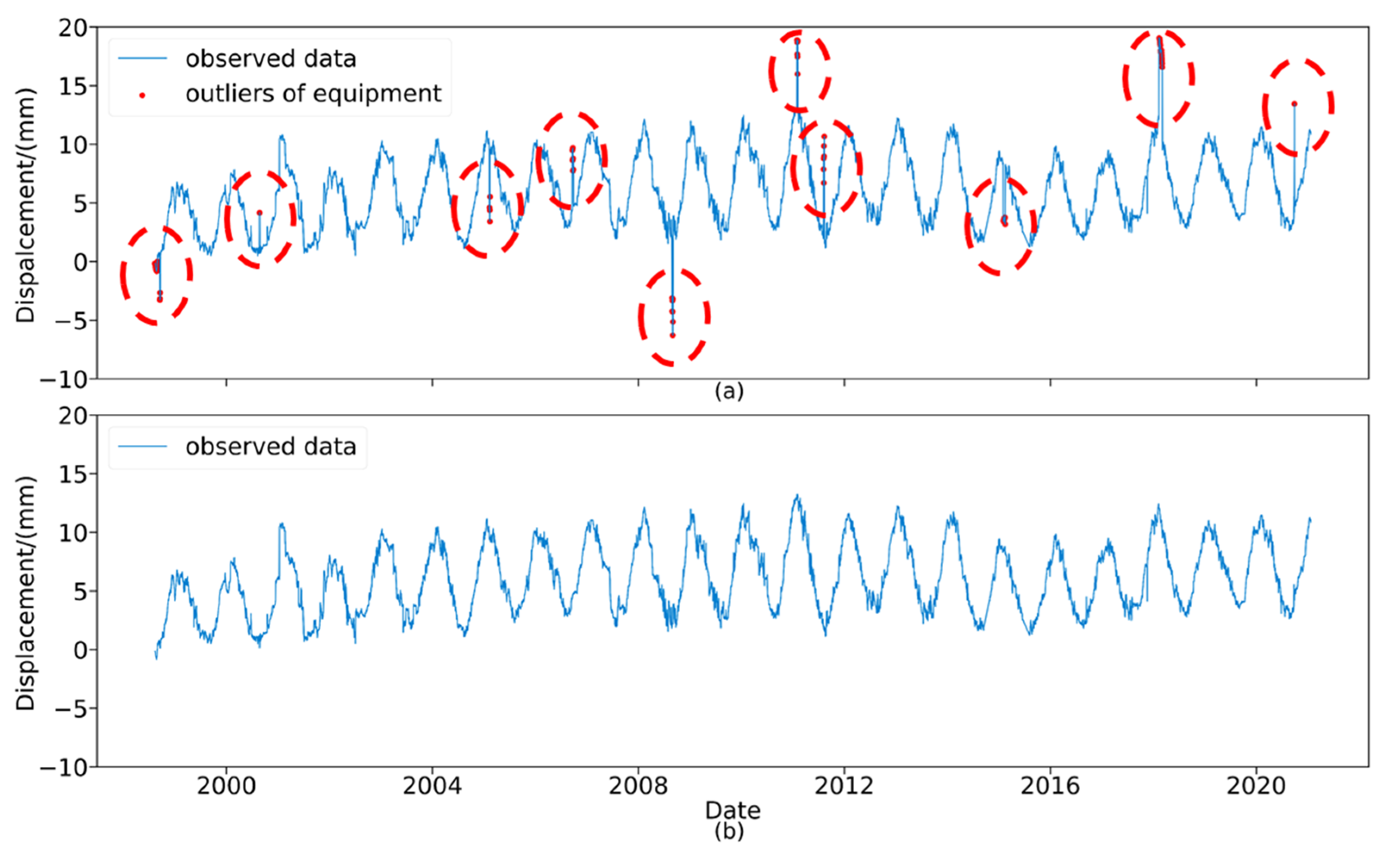
  • This paper proposed and tested a DBSCAN method to filter the dam deformation time series data. The method effectively removed the equipment based abnormal values caused by environmental factors or equipment failures, thereby smoothing the random measurement errors in the observed data, which improved prediction accuracy.
  • The importance of input variables to the dam deformation prediction model was analyzed to interpret and evaluate the model. This resulted in a useful and efficient qualitative measure of dam deformation, which improved prevention and control of abnormal structural responses.
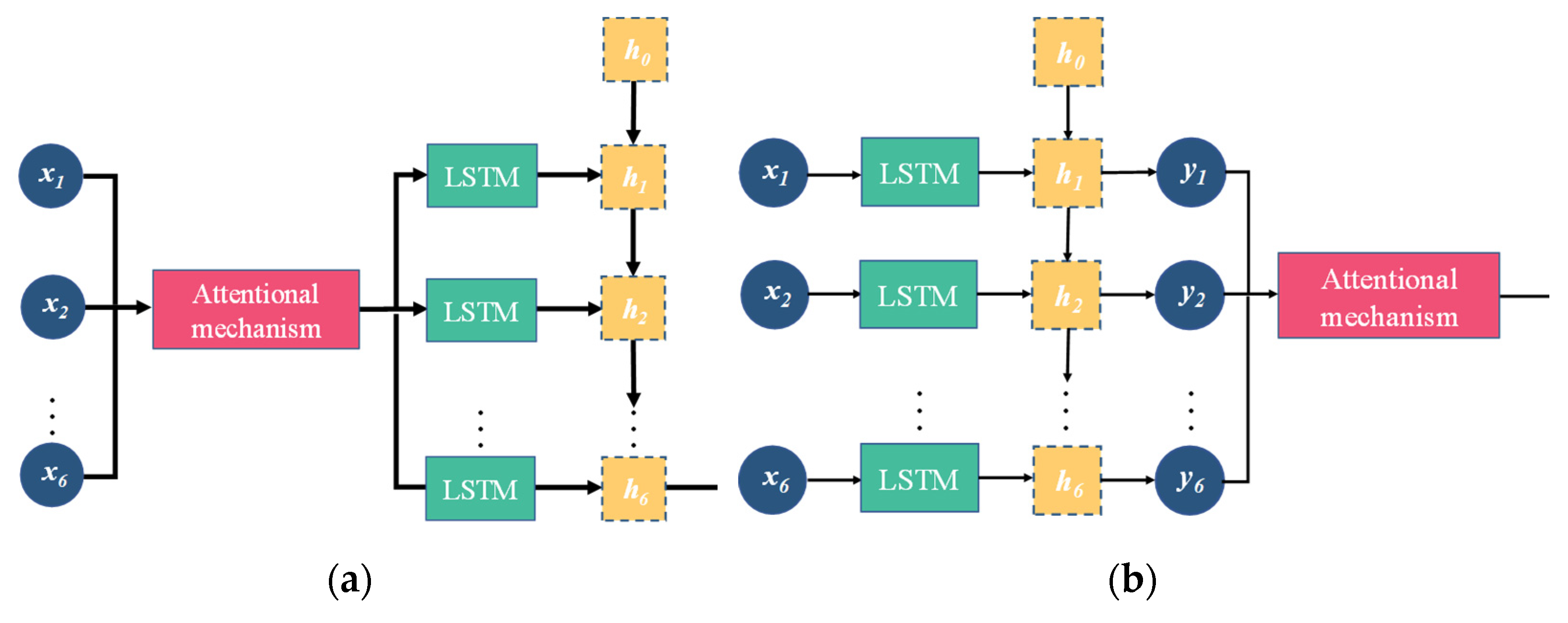
  • A coupled model was developed to better address the needs of dam deformation prediction. An attention mechanism focuses on the important variables in the short-term time dimension, while the LSTM model captures long-term change characteristics. This algorithm is very suitable for the prediction of dam deformation by accounting for time lag.
The remainder of this paper is organized as follows: Section 2 describes the detailed process of the established mathematical model of dam deformation and the preprocessing method. Section 3 introduces the selection of input variables, and the design and operation of the comparative experimental model. Section 4 elaborates on a case study from which actual monitoring data was collected. Section 5 explains and analyzes the input variables and evaluates the performance of the proposed coupled method. Finally, conclusions and future research directions are provided in Section 6.

2. Methods

2.1. Modeling Dam Deformation

Dam deformation is a key indicator reflecting the structural health of the dam. During project operation, polynomial functions are often used to approximate the dam deformation as:
δ = δ H + δ T + δ θ
where δ denotes the dam deformation, and the subscripts H , T , and θ in the formula respectively represent the components of the dam deformation caused by hydrostatic pressure, temperature, and aging effect over time.

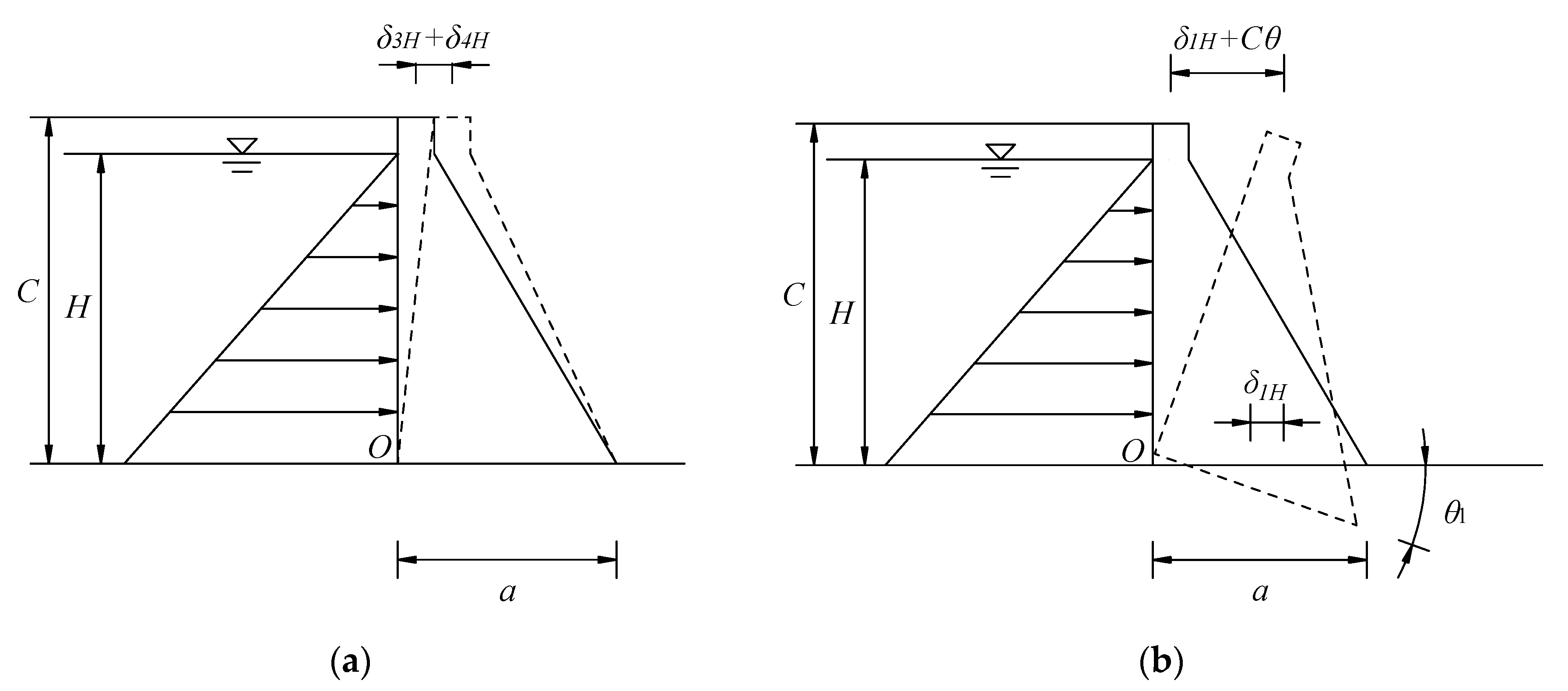
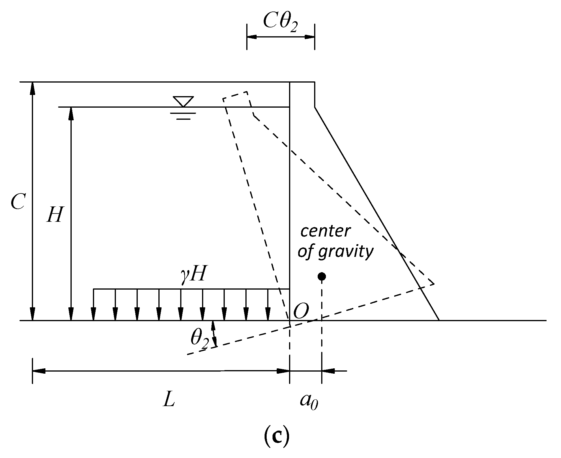
2.1.1. Hydrostatic Pressure Component

A simplified two-dimensional model of a homogeneous gravity dam is taken as an analysis example, as shown in Figure 1, we obtain the following explanation through the mechanical relationship between water level and deformation. Under hydraulic load, the horizontal displacement δ H generated at any measuring point of the dam is composed of four parts, as shown in Figure 1: the displacement δ 1 H caused by the deformation of foundation due to internal forces on foundation surface and the displacement δ 2 H caused by rotation of foundation surface due to the gravity of the reservoir water, the displacement δ 3 H caused by the rotation of reservoir water pressure acting on dam body, and the shear horizontal displacement δ 4 H caused by the internal force of reservoir water pressure acting on dam body. Therefore, the dam deformation is expressed by:
δ = δ 1 H + δ 2 H + δ 3 H + δ 4 H
According to F.Vogt theory [26], the water pressure to the bottom of a dam causes the horizontal displacement δ 1 H and rotation angel θ 1 of dam foundation as:
δ 1 H = ( γ K 1 / 6 E f a ) H 3 + ( γ K 2 / 2 E f ) H 2
θ 1 = ( γ K 3 / 6 E f a 2 ) H 3 + ( γ K 1 / 2 E f a ) H 2
where E f denotes the elastic modulus of bedrock; γ is unit weight of water; the width of dam bottom is a ; H presents the upstream water depth; and K 1 , K 2 , and K 3 are the coefficients that depend on the Poisson’s ratio of the bedrock and the length-to-width ratio of the equivalent rectangle at the bottom of the dam [27].
If the length of the reservoir L is very large, the weight of water acting on reservoir in front of dam will deform reservoir bank and cause rotation θ 2 at the bottom of dam as:
θ 2 = - H ( 1 + μ f ) ln ( n + n 2 + 1 ) / π E f
where μ f is the Poisson ratio of bedrock and n is half the ratio of the width of water in front of dam to the distance a 0 from the center of gravity of the dam to the heel of the dam.
Therefore, the horizontal displacement δ 2 H of crest caused by rotation of dam foundation θ as:
δ 2 H = c θ = ( θ 1 + θ 2 ) c
The horizontal displacement δ 3 H of dam crest caused by the rotation θ 3 of dam body as:
δ 3 H = 0 c 0 c M d y d y / E d I
where M = γ H 3 / 6 is the bending moment caused by water pressure, which is proportional to the third power of water depth; E d is the elastic modulus of dam concrete material; I is the moment of inertia of the horizontal section of dam and c is dam height.
The dam shear horizontal displacement δ 4 H as:
δ 4 H = 0 c 2 k ( 1 + μ d ) Q d y / A E d
where Q = γ h 2 / 2 is shear force caused by water pressure, which is proportional to the third power of the water depth; A is the horizontal area section of dam; k is the shear force distribution coefficient on the section, about 1.2; and μ d is the Poisson’s ratio of the concrete material of dam.
From the above analysis, it can be found that the horizontal displacement of dam crest caused by the water depth H in front of the dam is a function of H, H², and H³. Among them, the deflection displacement caused by the bending moment M is mainly related to H³, the tangential displacement caused by the shearing force Q is mainly related to H², and the slope-deflection at the tilt of reservoir bottom caused by the weight of water is related to H. Therefore, the hydrostatic pressure component in the horizontal displacement of a concrete gravity dam can be established as a mathematical model as follows:
δ H = a 0 + i = 1 3 a i H i
where a0 and ai are regression coefficients.
In addition, if the downstream water level changes greatly and the upstream and downstream water level difference is not obvious, the impact of downstream water level on monitoring should be considered, as:
δ H = a 0 + i = 1 3 a 1 i H 1 i + i = 1 3 a 2 i H 2 i
where H1 is the water level of upstream and H2 is the water level of downstream.

2.1.2. Temperature Component

Dam deformation is also affected by temperature, which is the displacement caused by temperature changes in the concrete of dam and rock foundation. When the dam has been in service for many years, the hydration heat of the concrete material has been dissipated, and the internal temperature of the dam body reaches a quasi-stable temperature field. At this time, it only depends on the boundary temperature variation, and the temperature component presents a simple harmonic periodic change. In order to qualitatively analyze the temperature component, multi-cycle harmonics can be selected as a factor to simplify and simulate it as:
δ T = i = 1 2 [ b 1 i sin ( 2 π i t / 365 ) + b 2 i cos ( 2 π i t / 365 ) ]

2.1.3. Time Component

The time component is an irreversible component that developed in a certain direction with the passage of time. Under the influence of a variety of factors, the dam body and rock foundation undergo plastic deformation, which leads to the rapid change of the time-effect displacement at the initial stage and gradually stabilizes in the later stage. According to existing research, linear functions and logarithmic functions can be used to model with time effects as:
δ θ = c 1 t + c 2 ln t
where c1 and c2 are regression coefficients.

2.2. Density-Based Spatial Clustering of Applications with Noise

In practical engineering, sensor monitoring is usually subject to harmful factors such as harsh environments or network transmission errors, resulting in abnormal values of equipment in data information. The density-based spatial clustering of applications with the noise (DBSCAN) method is introduced to reduce these random errors and eliminate device outliers, which has been proven to be capable of handling large database [28,29,30]. The DBSCAN is a density-based clustering algorithm. It assigns any point to a specified radius area and calculates the total number of points in the area to obtain the density of the specified point. When the density is higher than the preset maximum point set threshold, these points will be constructed into clusters. Based on this concept, a huge feature space is grouped into multiple regions with high density, so as to achieve the purpose of screening out random outliers of the monitoring equipment. We choose the DBSCAN method because it has the ability to divide clusters of arbitrary shapes in the noise spatial database, such as linear, elliptical shapes, etc. The detailed process of DBSCAN is described in Algorithm 1, where n and m are the number of samples and clusters, respectively. k represents any observed data in the original data set. ki represents the i-th observed data in the original dataset. x represents the number of observed data existing in the radius of ki. N represents the set of all observed points in each cluster. y represents the number of observed data existing in the radius of ki’.
Algorithm 1 Equipment outlier filtering
Inputs: Dataset D ( n × 1 ) , radius ε, domain density threshold MinPts
Outputs: Density-based cluster set D C ( m × 1 )
 Marking k in D ( n × 1 ) as UNVISITED, k [ 1 , n ]
For k i in   D ( n × 1 ) :
  If ki is UNVISITED
   Marking ki as VISITED
   If x>= MinPts
    Create a new cluster C and add ki to C to form a list set N
    For each point ki’ in N
     If ki’ is UNVISITED
      Marking ki’ is VISITED
      If y>= MinPts and each one in y ∉ any cluster
       Adding them into C
      End if
     End if
    End for
   Else
    Marking ki as outlier
   End if
  End if
 End for

2.3. Variable Importance Measures

The artificial intelligence learning model is a training model similar to a black box, and there is usually a problem that it is difficult to understand the training meta-model. Therefore, we introduce the random forest (RF) algorithm to calculate the relative importance of any combination of variables. The RF can reduce the average impurity of input variables, which is a very important part to improve the accuracy and interpretability of model. The main idea of RF is to ensure that the weight of the corresponding input variable is output under the condition of all input variables after receiving a given input. In theory, this method can be applied to any kind of dam deformation monitoring tasks. The detailed steps of RF model to calculate the relative importance of variables are described in Algorithm 2, where x and y represent the number of impact factors and observed data, respectively. ξ is the number of combinations containing different numbers of variables, and each combination must contain at least one variable. Xα is the α-th input variable set. y ^ ( α ) represents the dam deformation prediction result obtained by Xα. N is the number of decision trees in the set random forest. y ^ i ( α ) is the dam deformation prediction result obtained by the i-th decision tree using Xα. y ¯ is the average value of the observed data for dam deformation.
Algorithm 2 Variable importance measure for predictive model interpretation
Inputs: Observed dataset X ( x × y ) , Y ( y × 1 )
Outputs: Variable relative importance V I
 Divide X into α sets of tensors, α [ 1 , ξ ]
For α = 1 , , ξ :
   y ^ ( α ) = f ( X α )
   σ α = i = 1 n | y ^ i ( α ) y ¯ | / n
End for
For α = 1 , , ξ :
   V I α = σ α / α = 1 ξ σ α × 100 %
 End for

2.4. Long Short-Term Memory Networks Couple with Attention

Long short-term memory (LSTM) networks can effectively capture the nonlinear characteristics of time series through storing historical data streams. However, due to the diversified complexity of dam deformation monitoring, the time lag of influencing factors is particularly prominent. For example, an increase in temperature or water level does not immediately lead to dam deformation, but a gradual process, which manifests as a delayed deformation response. This factor increases the complexity of dam deformation prediction in the time dimension, so this paper develops a dam deformation prediction method based on the attention mechanism coupled with LSTM model.
LSTM model is essentially a device that superimposes and stores information. It adjusts the destination of information in the model unit through the special structure called gate. LSTM model has three gate structures: the forget gate determines the information that needs to be removed in the current cell unit; the input gate determines which information in the newly input information fragment is updated to the current cell unit and the output gate collects the information memorized by the cell unit to obtain the final output result. The calculation process expression of each LSTM cell unit is as follows:
f t = σ ( W f [ h t 1 , x t ] + b f )
i t = σ ( W i [ h t 1 , x t ] + b i )
c ˜ t = tanh ( W c [ h t 1 , x t ] + b c )
c t = f t c t 1 + i t c ˜ t
o t = σ ( W o [ h t 1 , x t ] + b o )
h t = o t tanh ( c t )
where ft is the operating threshold of the forget gate at time t; ht is the output value of the network at time t; ht−1 is the output value of the network at time t−1; it is the operating threshold of the input gate at time t; c ˜ t is the candidate value that needs to be updated at time t; ct is the new cell unit state at time t; ot is the operating threshold of the output gate at time t; Wf, Wi, Wc, and Wo are the weight matrix of the forget gate, input gate, cell state, and output gate, respectively; bf, bi, bc, and bo are the bias of the forget gate, input gate, cell state, and output gate, respectively; and σ and tanh are the activation functions.
However, the conventional LSTM networks are unable to perform quantitative impact analysis on the input data. Thanks to the concept of attention mechanism, it can achieve the focus on key information. It imitates the way humans process information and enable the algorithm to focus on core variables by means of activation functions. Therefore, a novel LSTM algorithm structure is proposed, coupled with an attention mechanism to predict dam deformation. The attention mechanism adds a matrix with the same dimension as the input tensor, weights the hidden state in the time dimension, and then outputs the attention vector value of each time step. The attention mechanism can be added in two positions, in front of the LSTM layer and behind the LSTM layer, as shown in Figure 2. In actual application, the target series has a complex amount of information, so the position added by the attention mechanism should be selected according to the actual effect. The attention mechanism calculates the weight e t i in each time dimension, and outputs the attention weight a t i between zero and one through the activation function, as shown below:
e t i = V T tanh ( W s S t 1 + W h h t )
a t i = soft max ( e t i ) = exp ( e t i ) / k = 1 T exp ( e t k ) ( t = 1 , 2 , , T )
where S t 1 is the attention layer input at the time t−1, and VT and Ws are the weight matrices that can be trained.
Then, we use this matrix vector to multiply the value in the time dimension to get the input of hidden layer c t i and, then, we update the hidden layer state of the LSTM model together with the previous unit cell state. The calculation formula is as follows:
c t = k = 1 T a t k h k
S t = L S T M ( Y t 1 , c t , S t 1 )
where Y t 1 is the attention layer output at the time t−1.

3. Model Implementation

This section mainly introduces the specific realization of the coupled algorithm for dam deformation prediction requirements, as shown in Figure 3. Since it uses a large number of historical data samples to test its validity, it can provide guidance and suggestions for the use of actual projects. Meanwhile, the evaluation metrics of the model are introduced.

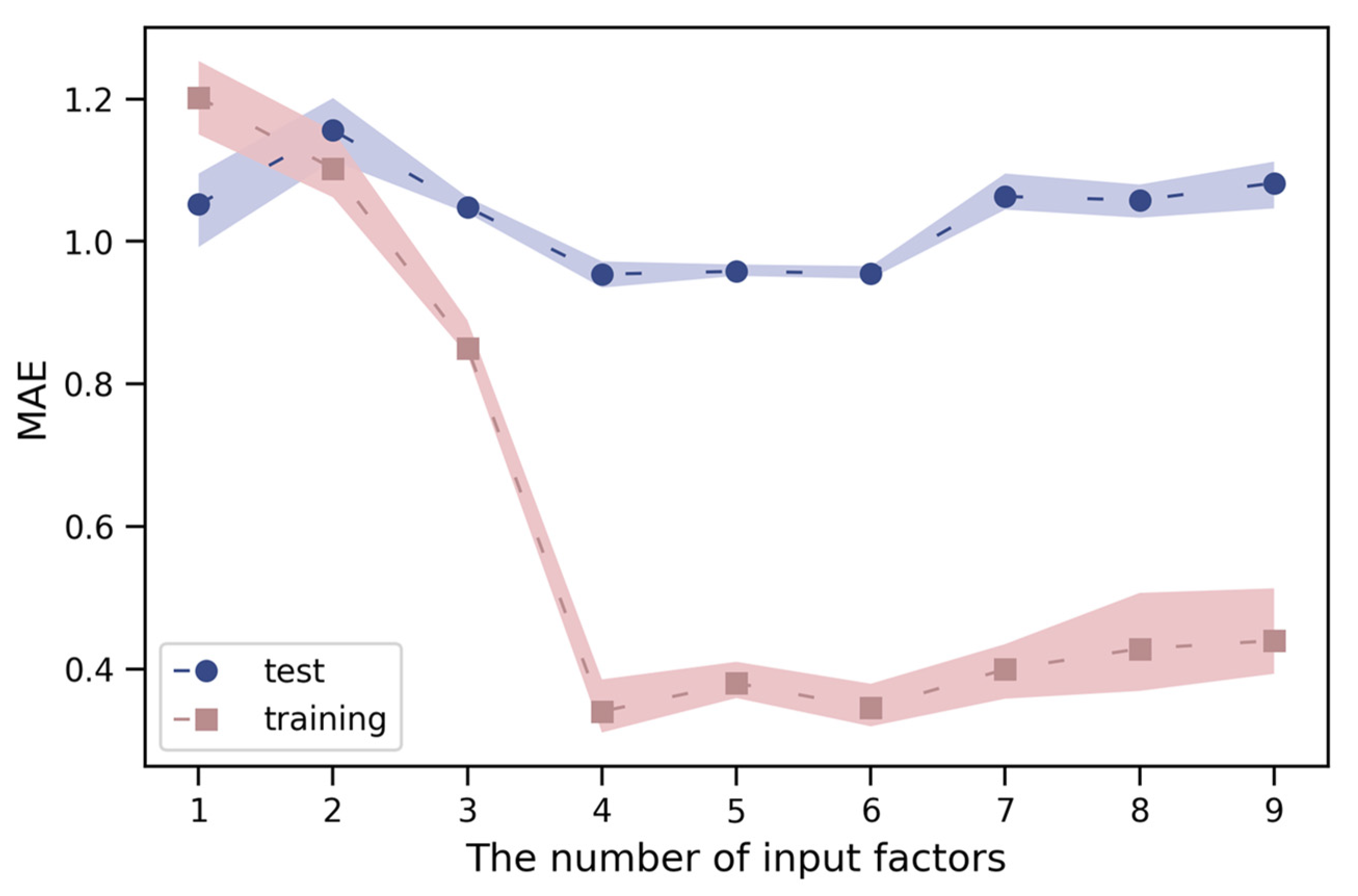
3.1. Selection of Input Variables

As discussed in Section 2.1. dam deformation is composed of water level component, temperature component and time component, so we consider these three components as input variables of the coupled model. Since the heat of hydration of the concrete material has been dissipated and the dam has a stable temperature field, the annual harmonic and half-year harmonic are used to express the temperature component. Finally, we generate a set of variables like Equation (23).
x = { H , H 2 , H 3 , sin ( 2 π / 365 ) , cos ( 2 π / 365 ) , sin ( 4 π / 365 ) , cos ( 4 π / 365 ) , θ , ln θ } = { H 1 , H 2 , H 3 , T 1 , T 2 , T 3 , T 4 , t 1 , t 2 }
In order to ensure the convergence of the coupled model or speed up its convergence, all input variables of Equation (23) need to be normalized as in Equation (24). Where μ is mean of sample data and σ is standard deviation of sample data.
x i = x i μ σ

3.2. Design of Comparison Schemes and Tuning Parameters

Design of a comparison scheme using eight algorithm models, these eight algorithm models are HST model, support vector machine using poly kernel (SVM-poly), support vector machine using radial basis function kernel (SVM-rbf), RF model, multilayer perceptron (MLP) model, standard LSTM, the attention mechanism is coupled to the model before LSTM layer, and the attention mechanism is coupled to the model after the LSTM layer. All of the algorithms are implemented in the Python 3.6 environment. The data processing is conducted with the Numpy and Pandas packages of Python. The modelling process using MLR, SVM, and RF is carried out using the package of Scikit-Learn in Python. Our MLP and LSTM networks are developed with Keras on top of Google TensorFlow.
For the HST model, it is essentially linear regression, and its regression coefficients are calculated by the least square method. For artificial intelligence models, each model has its own unique hyperparameters that need to be set. We introduce the method of grid search (GS) [31] to tune the hyperparameters on the data of training set. It arranges and combines the possible values of each hyperparameter from the pre-declared parameter interval, and lists all possible combinations to generate a grid. Then, use each combination for training and use ten-fold cross-validation to evaluate performance. After the fitting function has tried all the parameter combinations, a best hyperparameter combination is returned. SVM-poly model has two important parameters: the penalty coefficient C and the specified degree d. SVM-rbf model has two important parameters: penalty coefficient C and influence radius γ. RF model has three important parameters: the total number of trees n_estimators, the maximum number of features a single tree can have max_features and the minimum number of sample data owned by leaves min_sample_leaf. In order to suppress the overfitting phenomenon of LSTM and MLP models, it is necessary to add a dropout layer. Therefore, both the MLP and LSTM models have two important parameters: the number of hidden layer units u and the dropout rate. However, different from MLP, LSTM also needs to declare the size of the sliding time window w, which is how long the previous data needs to be considered when predicting the dam deformation in the next time period. Therefore, the partial autocorrelation function (PACF) of original dam deformation is calculated, as shown in Figure 4. It can be found that when the deformation lag is greater than eight, the values of PACF stabilize within the 95% confidence interval. Meanwhile, tuning the sliding time window size of the LSTM. When the optimal range of w is determined, testing the performance of the LSTM model with different values of w on the training set, and the results are shown in Figure 5. At first, due to insufficient effective information, the performance of model changes greatly. As the value of w increases, the model receives more information, which makes the performance of model gradually improve and eventually stabilize. Through Figure 4 and Figure 5, when the LSTM model uses a larger w, the performance of LSTM will not be affected by redundant information. In order to simplify the process of determining specific hysteresis of the impact factor, we can choose a larger w. The final experimental results are listed in Table 1.

3.3. Evaluation Criteria

To evaluate the performance of each model, the mean absolute error (MAE), root mean square error (RMSE), and maximum absolute error (AEmax) are selected as the evaluation indicators of models. The relevant calculation formulas are shown in Equations (25)–(27). For these three indicators, the smaller the value, the better the performance of the prediction model.
M A E = 1 n i = 1 n | y i y ^ i |
R M S E = 1 n i = 1 n ( y i y ^ i )
A E max = max | y i y ^ i | , i = 1 , 2 , , n
where n is the number of sample data, y i is the original dam deformation data, and y ^ i is the predicted dam deformation data.

4. Case Study

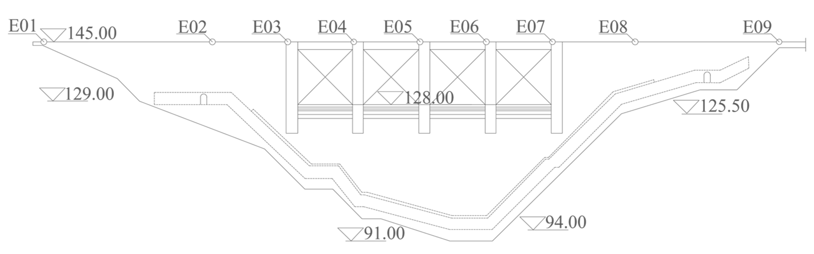
4.1. Case Description
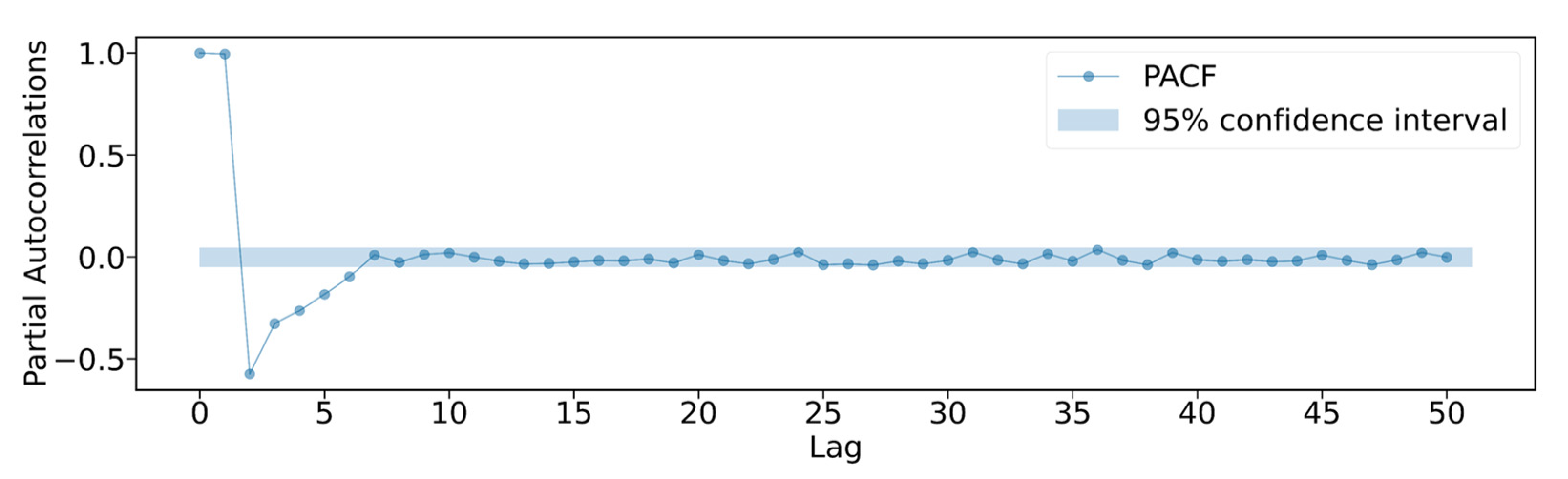
This study uses an integral roller compacted concrete gravity dam located in China as a case to verify the performance of the proposed coupled model. The dam axis is arranged in a broken line, the dam crest elevation is 145 m, the maximum dam height is 63 m, and the dam crest length is 196.62 m. The length of dam sections on the left and right banks are respectively 58.92 and 62.70 m, and there is a longitudinal drainage and grouting gallery in the dam body. The dam began to be closed for water storage in 1993 and passed the completion acceptance in 1995. In order to ensure the safe operation of the project, automatic monitoring equipment is used to continuously monitor the response of the dam structure. Meanwhile, for the realization of the horizontal displacement monitoring, nine measuring points are set on the top of the dam, numbered E01 to E09, as shown in Figure 6. The main distribution of measuring points is one on the left and right sections of the dam, two on the left and right abutments of the dam, five on the overflow section.
The environmental monitoring of water level is divided into upstream water level and downstream water level. The upstream water level measuring station is located in front of the upstream dam, and the downstream water level measuring station is located near the tail water outlet of the powerhouse. The upstream and downstream water levels are monitored in real time by self-registering water level gauges, supplemented by manual observation of water gauges.
Monitoring equipment collects data on dam deformation and related environmental variables once a day. In this study, since the E06 measuring point has the most obvious variation for the impact factor, it was chosen as an example for analysis. The DBSCAN method is used to preprocess the monitoring data from 1998 to 2021, and the dam deformation prediction performance of the proposed coupled model is studied.

4.2. Data Analysis

For the problem of dam deformation, it was first necessary to assess whether the influence of downstream water level should be considered. The data of the upstream and downstream water levels are presented in Figure 7. The downstream water level was generally stable compared to the upstream water level and the two water levels were quite different, so the influence of changes in the downstream water level were not included in the dam deformation model.
In addition to the standard dam related variables, there are many influencing factors that are difficult to remove, such as lightning strikes and interference by magnetic fields during monitoring. However, using the DBSCAN method to preprocess the observed data can effectively prevent equipment based abnormal values caused by such factors from contaminating the data set. The original observation data collected from the automated monitoring equipment are shown in Figure 8a, from which we can clearly find several equipment based abnormal values. The DBSCAN method uses clustering to identify equipment based outliers of the same level into a single category and then eliminate them. The results after removing the outliers can be seen in Figure 8b. The data processed through the DBSCAN method were smoother than the original observation data, and most of the abnormal values due to equipment error were eliminated.
The basic stats of the original data and the data processed using the DBSCAN method are listed in Table 2. The average values of the processed data were similar to the average values of the original data, but the standard deviation was reduced. This result showed that the DBSCAN method can effectively filter device caused outliers and help suppress any interference by such data on the prediction.

5. Results and Discussions

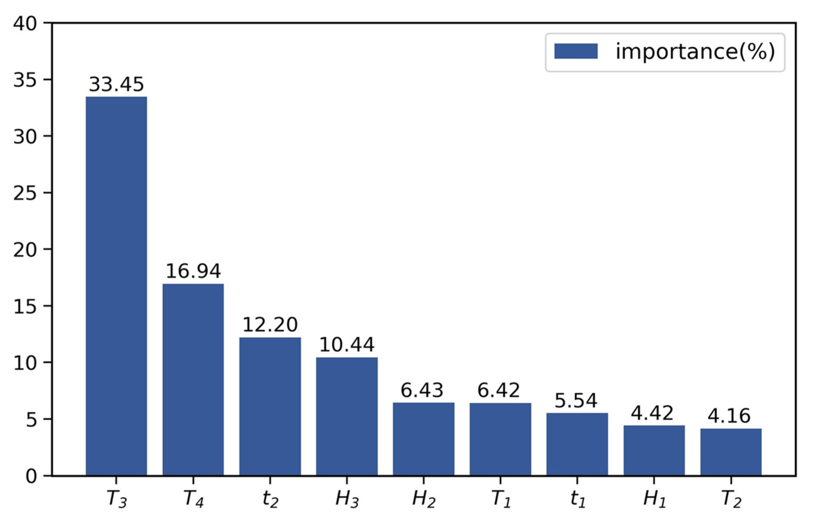
5.1. Importance of Input Variables and Model Interpretation

For a prediction model, the choice of input variables will directly affect the accuracy of the prediction results, so it needs to be determined if the input variables can fully represent the nonlinear relationship of dam deformation and whether the input variables are redundant. To do this we adopted the RF model to conduct a deep analysis of the input variables and determine the relative importance of each.
Figure 9 shows the relative importance of the nine input variables as calculated by the RF model using the GS method to optimize parameters. It can be seen that the temperature and water level factors were most relevant to dam deformation, with a relative importance of 60.97% and 21.29%, respectively. While the time component has the lowest bearing on the prediction results. From the perspective of hydraulic structural engineering, these calculated importance values demonstrated that temperature plays a central role in the deformation responses of dam structures, followed by water level, which is in line with the actual situation of the project and is reasonable. Although the time component had little influence on the model, the aging effect of the dam material and its inherent rheological characteristics may need to be analyzed as input variables to improve the nonlinear model.
Using the sequential backward selection method, the input variables are sorted from top to bottom according to importance. As can be seen from Figure 9, the order of importance of the input variables was T3, T4, t2, H3, H2, T1, t1, H1, and T2. In this order, the number of input variables fed to the RF model for training and testing is gradually increased. In order to meet the test requirements, 70% of the original data set is used as the training set and the remaining 30% data is used as the test set. Since the input sequence of the data set will also affect the test results, a ten-fold cross-validation is used to ensure the stability and reliability of the test results. The MAE values of the test results are provided in Table 3, and shown in Figure 10 to better visualize the different combinations. There were obvious fluctuations in the MAE values of the test and training sets at the beginning, and has not yet converged. This was because the model weighs the input variables and MAE values, and the effective information provided by the few input variables may not have been enough to represent the original time series. When the process continued and more variables were input, the MAE value significantly declined and the test set and training set began to stabilize. When using four, five, and six input variables, the MAE values of the test sets were basically stable at around 0.95, while those of the training set started to stabilize around 0.35. However, as the input variables continued to increase, the MAE values of the test and training sets increased again, and the increasing trend continued with additional variables. This was because the additional input variables contained redundant data that were not conducive to the prediction results, resulting in new features being captured by the model that contradicted those of the earlier data. Therefore, to ensure that the amount of information contained in the input variables is sufficient, while ensuring that MAE is as small as possible, a sixth plan should be selected to characterize dam deformation.

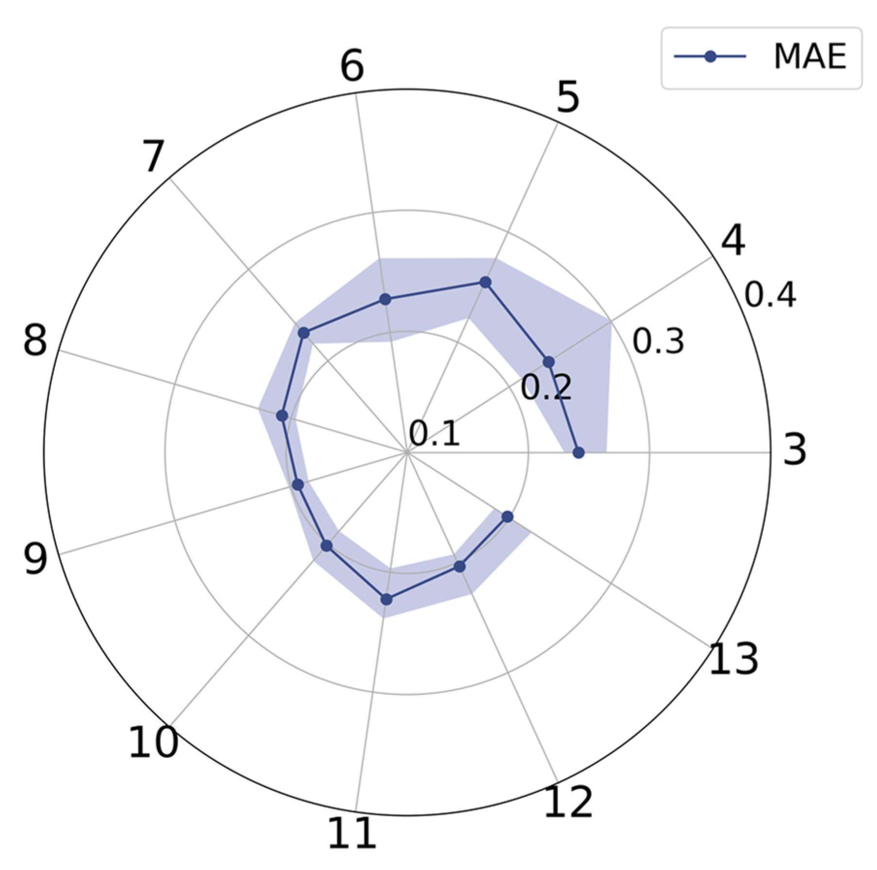
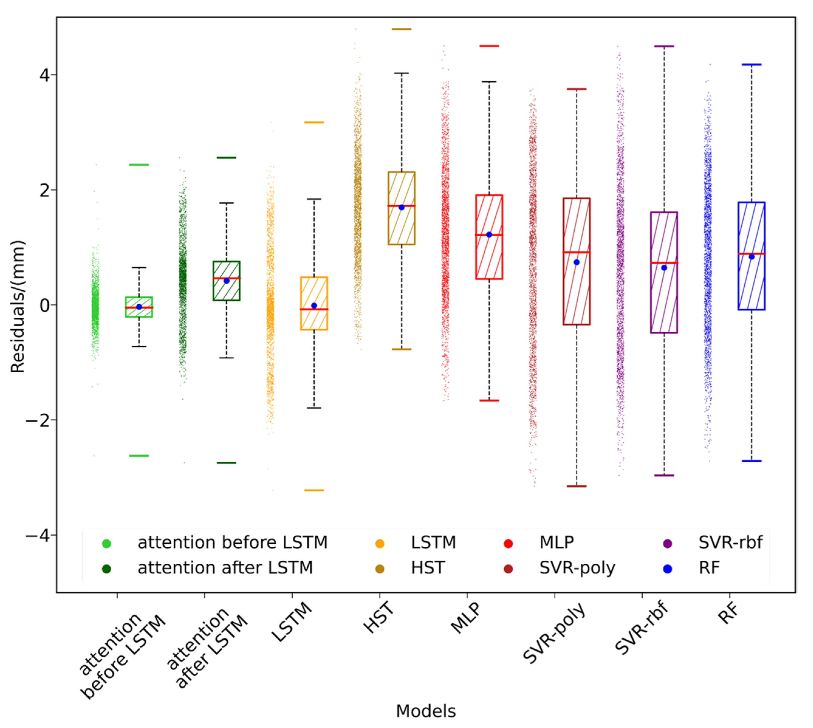
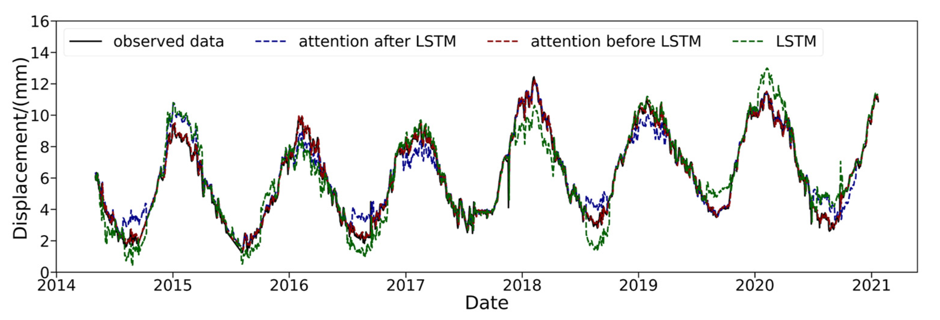
5.2. Performance of Prediction Accuracy and Interpretation in Time Dimension

The LSTM model coupled with the attention mechanism was compared to a variety of advanced algorithms. As was done for the proposed model, all models were trained with 70% of the original data set and tested with the remaining 30%. The evaluation index value of each model is listed in Table 4, where the best performing model is marked in bold. The evaluation indexes showed that, except for SVM-poly model which had too low a fitting accuracy for the high-dimensional data of the training set, all of the models fit the observation data well. The LSTM models exhibited the best fitting performances, and the model in which the LSTM layer was preceded by an attention mechanism performed better than all other models. The RMSE, MAE, and AEmax values of this model were all significantly lower than the other models, indicating its prediction results were the best.
To further compare the stabilities of the prediction results, the prediction residuals of all models were plotted, shown in Figure 11. The plot showed that the residual distribution of the HST model was right-skewed, and the prediction result gradually tended towards the average level of the training model over time. This was because linear fitting is more inclined towards the training data and does not consider non-linear effects of influencing factors, making linear fitting unable to accurately predict displacement caused by extreme weather. Although the distribution of the SVM-poly model was not skewed, its accuracy was not sufficient to meet the needs of dam deformation prediction through the median and quartiles. The SVR-rbf and MLP models showed improved prediction accuracy, but there were still problems with overfitting. The RF model did not exhibit overfitting, due to its own architecture, but it did exhibit generalization errors [32]. Therefore, the RF model had obvious right skewness, and would eventually tend to predict the average level like the HST model. Due to the introduction of time-dependent storage, the resulting LSTM has greatly improved the prediction accuracy and has a strong ability to represent nonlinear features, but it is still unable to predict peaks, as shown in Figure 12.
Meanwhile, in order to verify the reliability of the proposed model, drawing residuals plot of the better model, as shown in Figure 13. The results show that the proposed model has weaker residual autocorrelation than LSTM model, and its residual value distribution is more uniform. Although there are a few residual points of the proposed model on the residual graph with irregular distribution, most of residual points are evenly spread on both sides of 0. The residual distribution demonstrates unpredictability and randomness. Therefore, the LSTM model coupled with attention mechanism can fully capture the available information in the dam deformation influence factor.
The attention mechanism helps to automatically focus on important factors in the time dimension. This addition significantly improved the ability of the LSTM model to predict the peaks in the observed data. Furthermore, with the attention mechanism, the outliers in the forecasting data were relatively minor and the distribution of the residuals was also relatively concentrated. However, the attention mechanism performance depended on its coupling position, preceding or following the LSTM, and the results showed that when it is coupled before the LSTM layer it had better prediction accuracy. For dam deformation predictions, recent data has a stronger reference value and, as shown in Figure 14, attention disorder occurs when the attention mechanism is coupled after the LSTM layer. This is because after the data is processed by the LSTM layer it will be mapped into a complex high-dimensional tensor which makes it difficult for the attention mechanism to accurately focus on important factors. These observations demonstrated that the attention mechanism should be placed before the LSTM layer to better predict the structural response of dams using complex nonlinear factors and time delay information.

6. Conclusions

The accuracy of the dam deformation prediction algorithm is vital to dam safety monitoring. This paper proposed a coupled LSTM/attention mechanism model that used GS and cross-validation methods to adaptively identify the most important parameters. Real world monitoring data of deformations of a concrete gravity dam were used as the research object to test the model and its performance was compared with several other advanced methods. The RF model was used to calculate the importance of input variables and any extraneous influencing factors were screened out while maintaining a sufficiently reasonable description of the dam deformation response. In addition, abnormal data points caused by various factors interfering with the monitoring equipment were eliminated using the DBSCAN method. According to this comprehensive study, the following conclusions were drawn:
  • The results showed that the DBSCAN method is suitable for the detection of equipment based abnormal values. The processed data had an average value that was similar to that of the original data, but the variance and random errors were greatly reduced.
  • The RF model identified the most important variables needed to provide a reasonable explanation for dam deformation to be input into the model. The results revealed that the temperature was a particularly important factor in dam deformation, the importance of which was more than 50%, followed by water level, while the time component had the weakest influence.
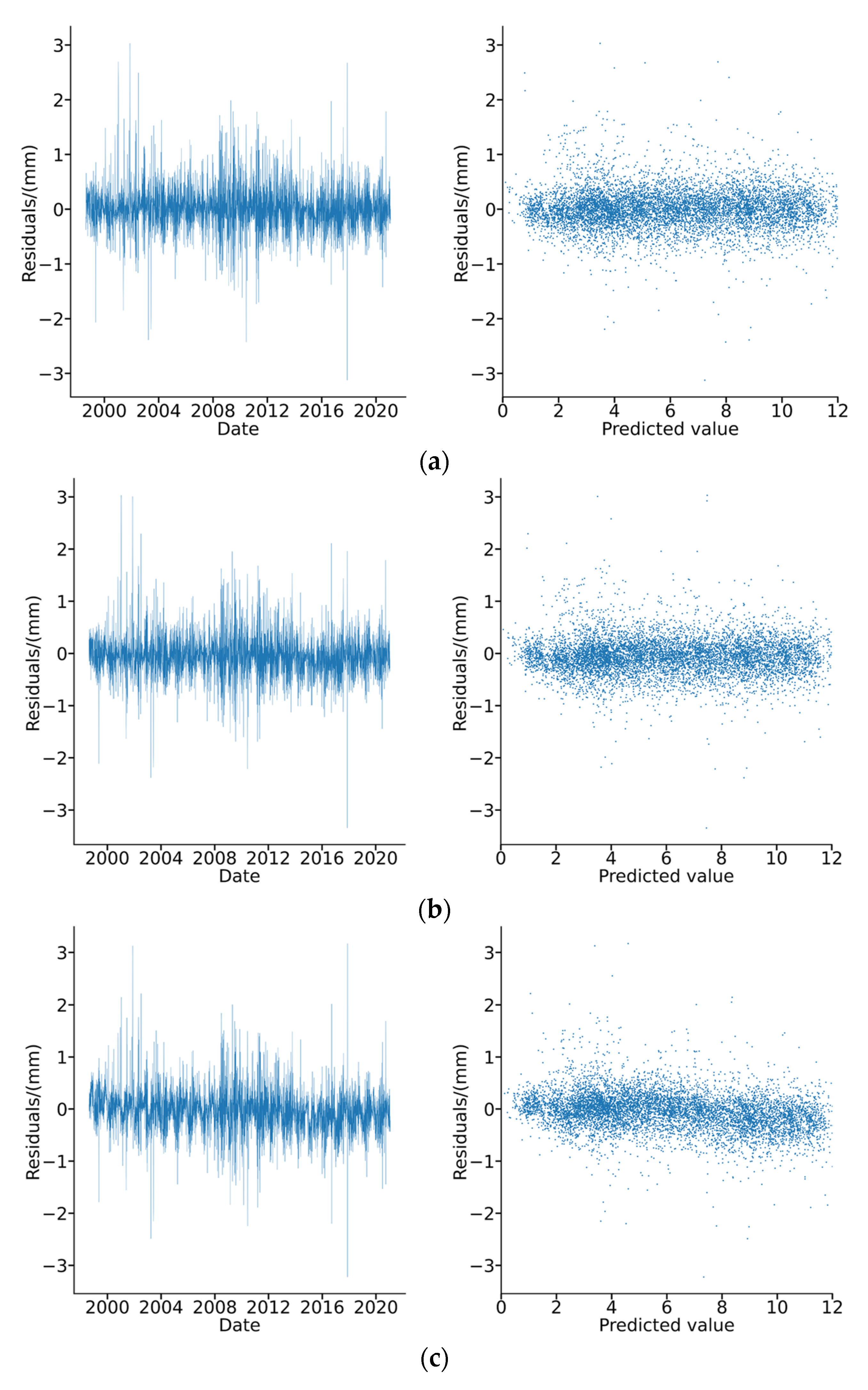
  • The time-lag effect in dam monitoring plays an important role in predicting dam de-formation. When the model contained a time sliding window, the accuracy of the results was significantly improved, the residual distribution was relatively concentrated, and the outliers were greatly reduced.
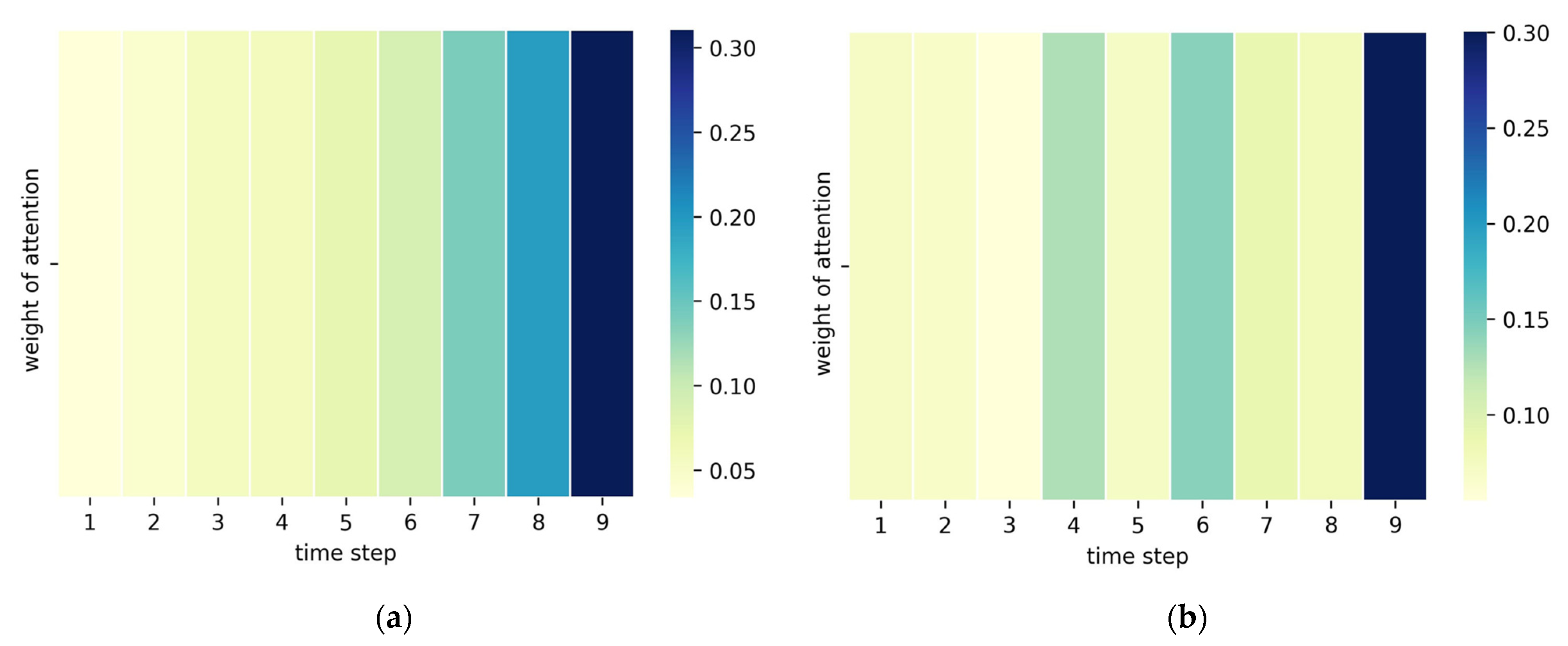
  • The addition of the attention mechanism enabled the model to focus on important factors in the time dimension and improved the prediction of extreme values. The attention mechanism should be added before the LSTM layer to prevent the high-dimensional mapping of data processed by the LSTM layer from causing attention disorder.
In the future, the effects of different normalization methods for input variables on the robustness of attention mechanism need to be discussed. Meanwhile, we will explore the dynamic effects of time lag and spatial characteristics of dam deformation to achieve coordinated dynamic predictions of dam deformation using multiple measurement points, which will analyze the dam safety as a whole and realize data reduction.

Author Contributions

K.W. conceived and designed the experiments and performed the modeling. Y.S. provided relevant technical support and produced the first draft. C.L. and Z.C. analyzed the data and reviewed and edited the paper. All authors discussed the basic structure of the manuscript and read and approved the manuscript. All authors have read and agreed to the published version of the manuscript.

Funding

This work was funded by the Young Scientist Program of Fujian Province Natural Science Foundation (Grant No. 2020J05108), and Talent Introduction Scientific Start-up Foundation of Fuzhou University (Grant No. 510890).

Institutional Review Board Statement

Not applicable.

Informed Consent Statement

Not applicable.

Data Availability Statement

Not applicable.

Acknowledgments

The authors would like to acknowledge the Electric Power Research Institute of State Grid Fujian Electric Power Co. Ltd. for dam deformation data.

Conflicts of Interest

The authors declare no conflict of interest.

References

  1. Cao, E.; Bao, T.; Gu, C.; Li, H.; Liu, Y.; Hu, S. A Novel Hybrid Decomposition—Ensemble Prediction Model for Dam Deformation. Appl. Sci. 2020, 10, 5700. [Google Scholar] [CrossRef]
  2. Lin, C.; Li, T.; Chen, S.; Liu, X.; Lin, C.; Liang, S. Gaussian process regression-based forecasting model of dam deformation. Neural Comput. Appl. 2019, 31, 8503–8518. [Google Scholar] [CrossRef]
  3. Willm, G.; Beaujoint, N. Les méthodes de surveillance des barrages au service de la production hydraulique d’Electricité de France, problèmes anciens et solutions nouvelles (The methods of surveillance of dams to serve hydraulic Production at Élec-tricité de France: Old problems and new solutions), Q34/R30. In Proceedings of the 9th International Congress on Large Dams (ICOLD), Istanbul, Turkey, 4–8 September 1967. [Google Scholar]
  4. Penot, I.; Daumas, B.; Fabre, J.P. Monitoring behaviour. Water Power Dam. Const. 2005, 57, 24–27. [Google Scholar]
  5. Mata, J.; Tavares de Castro, A.; Sá da Costa, J. Constructing statistical models for arch dam deformation. Struct. Control Health Monit. 2014, 21, 423–437. [Google Scholar] [CrossRef] [Green Version]
  6. Popovici, A.; Ilinca, C.; Ayvaz, T. The performance of the neural networks to model some response parameters of a buttress dam to environment actions. In Proceedings of the 9th ICOLD European Club Symposium, Venice, Italy, 10–12 April 2013. [Google Scholar]
  7. Mata, J. Interpretation of concrete dam behaviour with artificial neural network and multiple linear regression models. Eng. Struct. 2011, 33, 903–910. [Google Scholar] [CrossRef]
  8. Kao, C.Y.; Loh, C.H. Monitoring of long-term static deformation data of Fei-Tsui arch dam using artificial neural network-based approaches. Struct. Control Health Monit. 2013, 20, 282–303. [Google Scholar] [CrossRef]
  9. Ranković, V.; Grujović, N.; Divac, D.; Milivojević, N. Development of support vector regression identification model for pre-diction of dam structural behaviour. Struct. Saf. 2014, 48, 33–39. [Google Scholar] [CrossRef]
  10. Kang, F.; Li, J. Displacement Model for Concrete Dam Safety Monitoring via Gaussian Process Regression Considering Extreme Air Temperature. J. Struct. Eng. 2020, 146, 5019001. [Google Scholar] [CrossRef]
  11. Ren, Q.; Li, M.; Song, L.; Liu, H. An optimized combination prediction model for concrete dam deformation considering quantitative evaluation and hysteresis correction. Adv. Eng. Inform. 2020, 46, 101154. [Google Scholar] [CrossRef]
  12. Su, H.; Li, X.; Yang, B.; Wen, Z. Wavelet support vector machine-based prediction model of dam deformation. Mech. Syst. Signal Process. 2018, 110, 412–427. [Google Scholar] [CrossRef]
  13. Li, Y.; Bao, T.; Shu, X.; Chen, Z.; Gao, Z.; Zhang, K. A Hybrid Model Integrating Principal Component Analysis, Fuzzy C-Means, and Gaussian Process Regression for Dam Deformation Prediction. Arab. J. Sci. Eng. 2021, 46, 4293–4306. [Google Scholar] [CrossRef]
  14. Ren, Y.; Zhu, C.; Xiao, S. Small Object Detection in Optical Remote Sensing Images via Modified Faster R-CNN. Appl. Sci. 2018, 8, 813. [Google Scholar] [CrossRef] [Green Version]
  15. van der Burgh, H.K.; Schmidt, R.; Westeneng, H.-J.; de Reus, M.A.; Berg, L.H.V.D.; Heuvel, M.P.V.D. Deep learning predictions of survival based on MRI in amyotrophic lateral sclerosis. NeuroImage Clin. 2017, 13, 361–369. [Google Scholar] [CrossRef]
  16. Bello-Cerezo, R.; Bianconi, F.; Di Maria, F.; Napoletano, P.; Smeraldi, F. Comparative Evaluation of Hand-Crafted Image Descriptors vs. Off-the-Shelf CNN-Based Features for Colour Texture Classification under Ideal and Realistic Conditions. Appl. Sci. 2019, 9, 738. [Google Scholar] [CrossRef] [Green Version]
  17. Gelly, G.; Gauvain, J.-L. Optimization of RNN-Based Speech Activity Detection. IEEE/ACM Trans. Audio, Speech, Lang. Process. 2017, 26, 646–656. [Google Scholar] [CrossRef]
  18. Kim, M.J.; Cao, B.; Mau, T.; Wang, J. Speaker-Independent Silent Speech Recognition from Flesh-Point Articulatory Movements Using an LSTM Neural Network. IEEE/ACM Trans. Audio Speech Lang. Process. 2017, 25, 2323–2336. [Google Scholar] [CrossRef]
  19. Song, E.; Soong, F.K.; Kang, H.-G. Effective Spectral and Excitation Modeling Techniques for LSTM-RNN-Based Speech Synthesis Systems. IEEE/ACM Trans. Audio Speech Lang. Process. 2017, 25, 2152–2161. [Google Scholar] [CrossRef]
  20. Yuan, X.; Chen, C.; Lei, X.; Yuan, Y.; Adnan, R.M. Monthly runoff forecasting based on LSTM–ALO model. Stoch. Environ. Res. Risk Assess. 2018, 32, 2199–2212. [Google Scholar] [CrossRef]
  21. Su, Y.; Weng, K.; Lin, C.; Zheng, Z. An Improved Random Forest Model for the Prediction of Dam Displacement. IEEE Access 2021, 9, 9142–9153. [Google Scholar] [CrossRef]
  22. Liu, Y.; Guan, L.; Hou, C.; Han, H.; Liu, Z.; Sun, Y.; Zheng, M. Wind Power Short-Term Prediction Based on LSTM and Discrete Wavelet Transform. Appl. Sci. 2019, 9, 1108. [Google Scholar] [CrossRef] [Green Version]
  23. Liu, W.; Pan, J.; Ren, Y.; Wu, Z.; Wang, J. Coupling prediction model for long-term displacements of arch dams based on long short-term memory network. Struct. Control Health Monit. 2020, 27, e2548. [Google Scholar] [CrossRef]
  24. Qu, X.; Yang, J.; Chang, M. A Deep Learning Model for Concrete Dam Deformation Prediction Based on RS-LSTM. J. Sens. 2019, 2019, 1–14. [Google Scholar] [CrossRef]
  25. Xu, G.; Jing, Z.; Mao, Y.; Su, X. A Dam Deformation Prediction Model Based on ARIMA-LSTM. In Proceedings of the 2020 IEEE Sixth International Conference on Big Data Computing Service and Applications (BigDataService), Oxford, UK, 3–6 August 2020; Institute of Electrical and Electronics Engineers (IEEE): New York, NY, USA, 2020; pp. 205–211. [Google Scholar]
  26. Hartley, G.A.; McNeice, G.M.; Stensch, W. Vogt Boundary for Finite Element Arch Dam Analysis. J. Struct. Div. 1974, 100, 51–62. [Google Scholar] [CrossRef]
  27. Li, Z.Z. Dam Safety Monitoring; China Electric Power Press: Beijing, China, 1997; pp. 216–220. [Google Scholar]
  28. Zhou, A.; Zhou, S.; Cao, J.; Fan, Y.; Hu, Y. Approaches for scaling DBSCAN algorithm to large spatial databases. J. Comput. Sci. Technol. 2000, 15, 509–526. [Google Scholar] [CrossRef]
  29. Ester, M.; Kriegel, H.P.; Sander, J.; Xu, X. A Density-Based Algorithm for Discovering Clusters in Large Spatial Databases with Noise. In Proceedings of the 2nd International Conference on Knowledge Discovery and Data Mining KDD-96, Portland, OR, USA, 2–4 August 1996; pp. 226–231. [Google Scholar]
  30. Ester, M.; Kriegel, H.P.; Sander, J.; Xu, X. Clustering for mining in large spatial databases. KI J. 1998, 12, 18–24. [Google Scholar]
  31. Bergstra, J.; Bengio, Y. Random search for hyper-parameter optimization. J. Mach. Learn. Res. 2012, 13, 281–305. [Google Scholar]
  32. Breiman, L. Random forests. Mach. Learn. 2001, 45, 5–32. [Google Scholar] [CrossRef] [Green Version]
Figure 1. Schematic of the influence of hydraulic load on horizontal dam displacement: (a) horizontal displacement of dam foundation; (b) horizontal displacement caused by rotation of the dam foundation; and (c) horizontal displacement caused by dam rotation and shear horizontal movement. (unit: m).
Applsci 11 06625 g001aApplsci 11 06625 g001b
Figure 2. Schematic of the LSTM coupled with the attention mechanism: (a) attention mechanism preceding the LSTM layer and (b) attention mechanism following the LSTM layer.
Applsci 11 06625 g002
Figure 3. Flowchart of dam deformation prediction based on the coupled algorithm.
Applsci 11 06625 g003
Figure 4. The PACF results of the original observed data.
Applsci 11 06625 g004
Figure 5. MAE values of the LSTM model with different sliding time window size. The solid lines represent the average value from ten repeated simulations and the upper and lower boundaries of the band represent the maximum and minimum from the ten simulations.
Applsci 11 06625 g005
Figure 6. The layout of horizontal displacement measuring points on the dam.
Applsci 11 06625 g006
Figure 7. Water level data collected from automated monitoring equipment: (a) upstream water level and (b) downstream water level.
Applsci 11 06625 g007
Figure 8. Dam horizontal displacement data collected from automated monitoring equipment: (a) the original data and (b) the data processed through DBSCAN.
Applsci 11 06625 g008
Figure 9. The relative importance of input variables determined by the RF model.
Applsci 11 06625 g009
Figure 10. The MAE values of each group under ten-fold cross-validation.
Applsci 11 06625 g010
Figure 11. Comparison of the inherent stability and predictive performance of different models.
Applsci 11 06625 g011
Figure 12. Predictive fitting curve of the LSTM and coupled models.
Applsci 11 06625 g012
Figure 13. Residuals distribution plot of different models: (a) attention mechanism is coupled before LSTM; (b) attention mechanism is coupled after LSTM; and (c) LSTM.
Applsci 11 06625 g013
Figure 14. Heat map of attention weight: (a) the attention mechanism is coupled before LSTM and (b) the attention mechanism is coupled after LSTM.
Applsci 11 06625 g014
Table 1. Basic information of model parameter tuning.
ModelsHyperparametersSearch RangeOptimal ValueTraining: MAETest: MAE
SVM-polyC(15, 30)211.55041.3880
d[1,2,3,4,5]1
SVM-rbfC(15, 25)200.55981.2799
γ(0.1, 0.5)0.2
RFn_estimators(25, 40)290.39871.2282
max_features(0,1)0.5
min_sample_leaf[1,2,3,4,5]3
MLPu[64, 512]1280.65611.3364
Dropout rate[0.4–0.8]0.5
LSTMu(64, 521)2560.17520.2037
Dropout rate[0.4–0.8]0.5
w[3, 15]9
Table 2. Summary statistics of the original data and the data processed through DBSCAN.
AttributeThe Original DataThe Data Processed through DBSCAN
Max19.079113.2493
Min−6.2839−0.8423
Mean5.98066.0159
Median5.78285.7860
Standard3.08662.8342
Table 3. Evaluation of simulation results for different input factors.
Serial NumberSearch RangeMAE
T3T4t2H3H2T1t1H1T2TrainingTest
1 1.20221.0520
2 1.10231.1563
3 0.85051.0482
4 0.34050.9541
5 0.38020.9581
6 0.34530.9550
7 0.39901.0633
8 0.42801.0584
90.43921.0821
Table 4. Performance comparison of different models.
ModelTrainingTest
RMSEMAEAEmaxRMSEMAEAEmax
Attention before LSTM0.13370.12483.03040.04980.15352.6235
Attention after LSTM0.07580.18013.02950.06460.18462.7444
LSTM0.04980.17523.12690.07980.20373.1708
RF0.26620.39872.35402.20301.22824.1766
SVM-rbf0.57770.55982.75552.39691.27994.4931
SVM-poly3.32831.55044.00042.69431.38803.7492
MLP0.68580.65613.55702.59701.33644.5004
HST0.87140.74243.59003.65621.71424.7921
Publisher’s Note: MDPI stays neutral with regard to jurisdictional claims in published maps and institutional affiliations.

