Article

Neuro-Fuzzy Transformation with Minimize Entropy Principle to Create New Features for Particulate Matter Prediction

by
Krittakom Srijiranon
1 and
Narissara Eiamkanitchat
2,*
1
Department of Computer Engineering, Faculty of Engineering, Graduate School, Chiang Mai University, Chiang Mai 50200, Thailand
2
Department of Computer Engineering, Faculty of Engineering, Chiang Mai University, Chiang Mai 50200, Thailand
*
Author to whom correspondence should be addressed.
Appl. Sci. 2021, 11(14), 6590; https://doi.org/10.3390/app11146590
Submission received: 24 June 2021 / Revised: 8 July 2021 / Accepted: 14 July 2021 / Published: 17 July 2021
(This article belongs to the Special Issue Principles and Applications of Data Science)

Abstract

:
Air pollution is a major global issue. In Thailand, this issue continues to increase every year, similar to other countries, especially during the dry season in the northern region. In this period, particulate matter with aerodynamic diameters smaller than 10 and 2.5 micrometers, known as PM10 and PM2.5, are important pollutants, most of which exceed the national standard levels, the so-called Thailand air quality index (T-AQI). Therefore, this study created a prediction model to classify T-AQI calculated from both types of PM. The neuro-fuzzy model with a minimum entropy principle model is proposed to transform the original data into new informative features. The processes in this model are able to discover appropriate separation points of the trapezoidal membership function by applying the minimum entropy principle. The membership value of the fuzzy section is then passed to the neural section to create a new data feature, the PM level, for each hour of the day. Finally, as an analytical process to obtain new knowledge, predictive models are created using new data features for better classification results. Various experiments were utilized to find an appropriate structure with high prediction accuracy. The results of the proposed model were favorable for predicting both types of PM up to three hours in advance. The proposed model can help people who are planning short-term outdoor activities.

1. Introduction

Air pollution is a major problem in public health that increases health impacts on both the cardiovascular and respiratory systems in humans [1]. There are many important air pollutants, including ground-level ozone (O3), carbon monoxide (CO), nitrogen dioxide (NO2), sulfur dioxide (SO2), and particulate matter (PM), announced by the World Health Organization. However, PM exceeds both the national and international standards to the greatest extent compared with others [2]. The PM is a mixture of particles that it compounds and four types of components, namely, organic, inorganic, biological, and carbonaceous materials. The proportion of each component is different in each area [3]. Most of the PM is classified into two categories by size, which are based on health-related effects [4]. The size of PM affecting human health has an aerodynamic diameter of less than 10 μm, which can only be detected by an electron microscope. There are two major sizes of PM. First, coarse particulate matter called PM10 is PM with an aerodynamic diameter smaller than 10 μm. Another type is fine particulate matter called PM2.5, which is PM with an aerodynamic diameter smaller than 2.5 μm [5,6]. However, there are other types of PM, such as PM1 [7], which are excluded from this research due to air pollution standards.
Every year during the dry season, which begins in February, the upper northern region of Thailand is affected by air pollution problems from both types of PM and this problem ends when the rainy season begins [8]. Anthropogenic activities, both garbage and agricultural burning, are important sources that contribute to air pollution. After the harvest periods, farmers prepare their area for the next crop period by burning their crop residues [9]. Another source is wildfire from natural and human-made occurrences as this area is mostly covered with forests and mountains. Fire management is difficult due to many limitations, such as a lack of effective equipment [10]. There are many policies from the government to protect and prohibit burning. However, the air pollution problem does not seem to be improved.
In recent years, researchers have been focused on both processes and methods in data science to apply it in various applications, such as daily cattle health classification [11], tomography image analysis [12], and student dropout prediction [13]. For the air pollution problem, data science techniques can implement notification systems to alert people by predicting the upcoming air pollution level. Numerous research articles are interested in applying data science to the air pollution problem, especially both types of PM. They try to find both appropriate processes and methods to create prediction models with high model performance or computation time reduction for their desired output, such as PM concentrations, PM levels, or classes [14,15,16]. The popular models are multiple linear regression (MLR), autoregressive integrated moving average (ARIMA), and various types of artificial neural networks (ANNs).
MLR is a popular statistical model for comparing the model performance with the ANN, but the results showed that MLR is less effective than ANN [17,18,19,20]. ARIMA is a common model for time-series data. There are two interesting examples. The first example, a combination of MLR and ARIMA proposed by [21] was used to predict daily and monthly average PM10 concentrations in Delhi, India. The second example, using the output data from ARIMA as input features for MLR, was presented by [22]. In the article, ARIMA is used with the dataset, including seasonal features and the period of seasonal patterns, to predict hourly PM10 concentrations in Negeri Sembilan, Malaysia.
The ANN is the most popular model selected by many researchers as it outperforms other models. The presentation in [23] focusing on three cities of China proposed a combination of the rolling mechanism and gray model in the data preparation process and the ANN model was used in the prediction process. The result was a prediction of the daily average values of PM10 concentrations and PM10 classes, calculated from the China air quality index. A research article presented in [24] applied ANN to predict the highest daily PM10 concentration in Santiago, Chile. The rule-based classification is used from a combination of two models, ANN and K-nearest neighbor (K-NN), to improve model performance in the minor classes. There is another type of ANN, long short-term memory (LSTM), used by [25]. The research presented an appropriate LSTM structure to predict the daily average PM10 concentration in Seoul, South Korea.
Another type of ANN is a combination of ANN and fuzzy logic called neuro-fuzzy. Two research articles used neuro-fuzzy with the Tagaki-Sugeno system to predict daily average PM10 concentrations in Turkey. The output data from fuzzy logic was used as an input feature for ANN. In the fuzzy logic part, in [26], a bell-shaped membership function was selected, while in [27], the Gaussian membership function was selected. Moreover, neuro-fuzzy is more effective than the other classifiers, such as NN and the support vector machine, when using the standard datasets from UCI reported by [28,29,30]. Neuro-fuzzy was selected to be applied in various applications, such as the diffuse large B-cell lymphomas classification [31]. In addition, in [32], it was reported that the positions for changing slope in the fuzzy membership function are very important, so the minimum entropy principle (MEP) is applied to find these values.
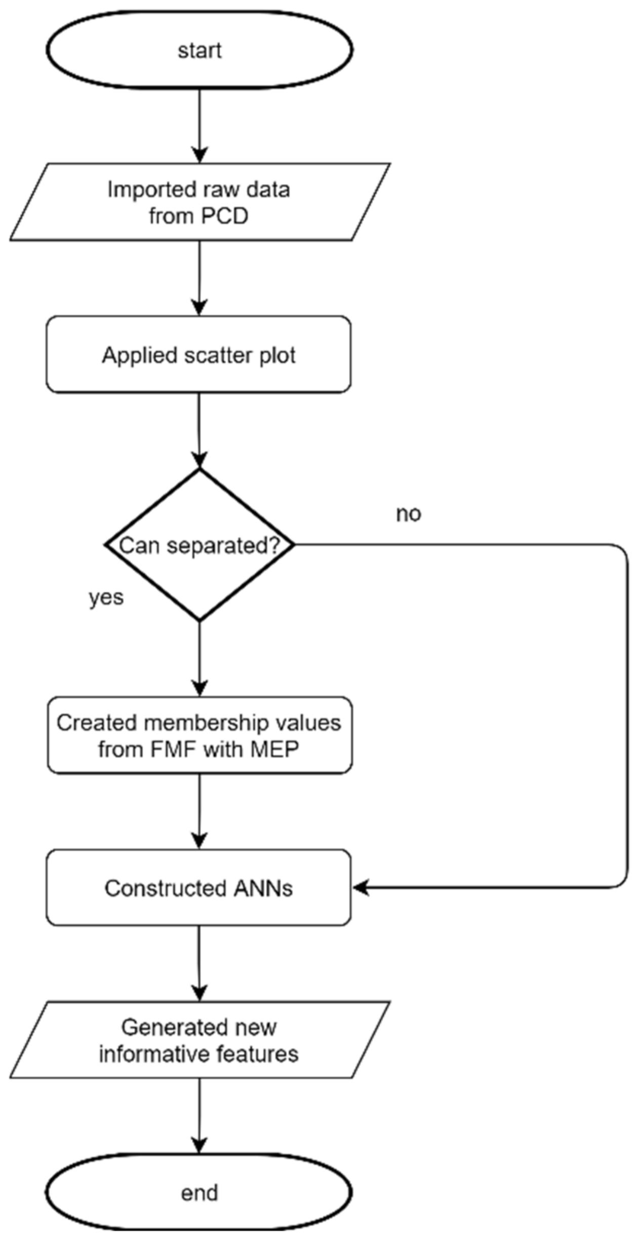
This research proposes the neuro-fuzzy with the minimum entropy principle model for data transformation to create new informative features that are used to represent historical data. Moreover, the proposed transformation model can reduce concerns about bias in raw data. Finally, an ANN model is created for new informative features. The three- and five-class output data of this model are the hourly PM10 and PM2.5 classes associated with the Thailand standard. The results of the model can be an application implemented to alert people and for short-term outdoor activity planning up to three hours in advance.

2. Materials and Methods

This section is divided into three subsections. The first subsection presents the details of the research areas and air quality standards in this research. The second subsection proposes the structure of the proposed model to create new informative features. The third subsection discusses the details of the prediction model to classify both types of PM.

2.1. Thailand Air Quality Index

The study area of this research is the upper northern part of Thailand due to the air pollution problem during summer every year. This area includes 8 provinces: Chiang Mai, Chiang Rai, Lampang, Lamphun, Mae Hongson, Nan, Phayao, Phrae, and Uttaradit. Only fixed-site data monitoring stations from the Pollution Control Department (PCD), Ministry of Natural Resources and Environment, Thailand, were selected to create a prediction model.
There are 14 fixed-site data monitoring stations in total; each province except Uttaradit has at least one station. The timing of raw data from these stations differs depending on the availability of recorded data from each location. However, the first date for most of the recordings is 1 January 2010 and the recording end date is 30 April 2018 (for additional details, see Appendix A). Considering the completeness of data, only one station per province was selected from all stations. Therefore, there were eight fixed-site data monitoring stations used in this research as follows:
  • Yupparaj Wittayalai School, Chiang Mai (CHM-Yup);
  • Natural Resources and Environment Office, Chiang Rai (CHR-Env);
  • Lampang Meteorological Station, Lampang (LPA-Met);
  • Provincial Administrative Stadium, Lamphun (LPH-Sta);
  • Natural Resources and Environment Office, Mae Hongson (MHS-Env);
  • Chaloem Phra Kiat Hospital, Nan (NAN-Hos);
  • Knowledge Park, Nan (NAN-Hos);
  • Phrae Meteorological Station, Phrae (PHA-Met).
Data from PCD were divided into two groups. The first group was meteorological, including wind speed (WS), wind direction (WD), relative humidity (RH), pressure (PR), rain (RA), temperature (TEMP), and solar radiation (SR). The other group was air pollution data, including PM10, PM2.5, ground-level ozone (O3), carbon monoxide (CO), nitrogen monoxide (NO), nitrogen dioxide (NO2), and sulfur dioxide (SO2). Each station records different parameters (for additional details, see Appendix B). According to the investigation, it was found that 6 out of 8 stations with almost all parameters were collected, except PM2.5, available in only two stations: CHM-Yup and NAN-Hos. In addition, the rain was excluded as an input feature in all data monitoring stations due to numerous zero values with more than 99% during the focus period of the experiment.
To report the levels of air pollution for people, an air quality index was used. Air pollution concentrations were divided into groups and represented by the color scheme. The number of groups and the range of concentrations in each group differed according to the law of each country. In Thailand, the PCD under the Thai government announced the Thai air quality index (T-AQI) [33] as a standard for classifying air quality. This index selects six air pollutions, namely, PM10, PM2.5, O3, CO, NO2, and SO2. In T-AQI calculations, each air pollution was transformed to the T-AQI level by the corresponding equation, then the final T-AQI level reported to people was identified from the maximum value of T-AQI. Both types of PM often have the highest T-AQI levels compared to the other four air pollutions, so this research selected only two types of PM to create a prediction model. There are five groups of T-AQI; therefore, the meaning and ranges of each group were calculated from concentrations of both types of PM, as shown in Table 1.

2.2. The Neuro-Fuzzy Transformation with Minimum Entropy Principle Model

Data transformation is an important process in data science. This research proposes a neuro-fuzzy with minimum entropy principle (NFT-MEP) model for a novel data transformation. The flowchart of the proposed model is displayed in Figure 1, divided into four processes. First, the raw data from PCD used extract–transform–load (ETL) to create the dataset. This process used the scatter plot to divide input features into two groups. The first group is input features that can apply the fuzzy membership function (FMF) as Dataset-I and the second group is input features that cannot apply FMF as Dataset-II. Therefore, two datasets were created from ETL. Second, the minimum entropy principle was used to find the optimal positions of each FMF from Dataset-I and then membership values were created as Dataset-III. Third, both Dataset-II and Dataset-III were combined and then neural network (NN) models were utilized to output data. Finally, new informative features were generated from the output of the previous process. The additional details of each process are represented in each subsection.

2.2.1. Extract–Transform–Load

The raw data from the PCD in each fixed-site data monitoring were received from different sensors, so all of them were extracted into a database and each database represents one station. Next, missing values were eliminated from the raw data. Each input feature was then considered to prepare for transformation. Scatter plots were utilized to input all features. They can determine the appropriate input features that can be transformed into membership values. The x-axis represents records of raw data and the y-axis represents the values of the input feature, while the colors of points represent the classes of PM. Considering that in each scatter plot, there is only one input feature that the distribution can separate from each color of the classes, it would be appropriate to use FMF to create membership values as Dataset-I. On the other hand, for an input feature that the distribution cannot separate from each color of the classes, the original value was used as Dataset-II. Finally, both Dataset-I and Dataset-II were loaded into the next process.
For example, the scatter plot of two input features from the LPA-Met station are shown, RH in Figure 2a and CO in Figure 2b, to filter out the appropriate features. This station contains approximately 16,000 records of raw data. The colors blue, red, and green, were used to represent three classes of the output data, Class 1, Class 2, and Class 3, respectively. As seen in Figure 2a, the scatter plot of the RH values and classes were difficult to separate from each other. On the other hand, the colors of the CO in Figure 2b were relatively separate. First, the blue color was mostly a CO value below 1. Second, the red color was mostly a CO value between 0.5 and 1.5. Finally, the green color was mostly a CO value above 1. Therefore, RH was loaded into Dataset-II, while CO was loaded into Dataset-I.

2.2.2. Fuzzy Membership Function with Minimum Entropy Principle

Fuzzy logic is based on uncertainty and an unsharp boundary that can be applied in some real-world applications. A difference between Boolean logic and fuzzy logic is that Boolean logic is a set of two values, completely true or 1 and completely false or 0. On the other hand, fuzzy logic is a fuzzy set including an infinite value between partial false or 0 and partial true or 1. Values in a fuzzy set called membership values are calculated by an FMF. This research selected trapezoidal functions as the FMF. Each input feature can include one or more FMFs and the number of FMFs of each input feature is two to five functions.
To find the optimal positions of the changing slope on the FMF, the minimum entropy principle (MEP) was used. This method finds the minimum value of entropy, which is an uncertainty of the data. The high entropy value means that there is a high probability that cannot divide data between classes. To find MEP, the threshold (x) in a range between X1 and X2 was calculated by Equations (1)–(3). This threshold divided data into two sides: the left side in [X1, x] as side p is calculated by Equation (1) and the right side in [x, X2] as side q is calculated by Equation (2). Then, x was gradually adjusted to the values between X1 and X2 to find the minimum entropy from Equation (3) and its value is the lowest entropy of data divided into two sides in ranges [X1, x] and [x, X2] [34].
S p x = i = 1 2 p i x ln p i x
S q x = i = 1 2 q i x ln q i x
S x = p x S p x + q x S q x
where S(x) denotes the entropy value of x in range X1 and X2; p(x) and q(x) denote probabilities that all samples are in range [X1, x] and [x, X2], respectively; p(x) + q(x) = 1, pi(x) and qi(x) denote conditional probabilities that class i sample is in range [X1, x] and [x, X2], respectively.
After finding the minimum entropy as x m i n , this value was used to determine the positions of the changing slope on the trapezoidal function by applying MEP again to find x L and x H . The x L is a threshold with the minimum entropy in the range X 1 , x L and x L , x m i n , while x H is a threshold with the minimum entropy in range x m i n , x H and x H , X 2 . Finally, x L and x H are separate points of the trapezoidal function. Next, the FMF was applied and each parameter has three to five new input features from the membership values.
Dataset-I from the ETL process applied FMF with MEP to create Dataset-III. For example, the CO in Figure 2b was applied to the MEP twice. The first MEP was used to divide between Class 1 and Class 2, while the second MEP was used to divide between Class 2 and Class 3. The first MEP results showed that x L and x H were 0.75 and 1.05 with the minimum entropy values 0.5165 and 0.6584, respectively. In addition, the second MEP results showed that x L and x H were 1.15 and 1.45 with the minimum entropy values 0.5595 and 0.4230, respectively.
This feature was divided into three FMFs. The membership values of each membership function were calculated from Equations (4)–(6) for low, medium, and high, respectively, where μ denotes the membership value and x denotes an input feature. In addition, Figure 3 shows a graph of three trapezoidal membership functions of the CO.
μ L o w x = m a x m i n 1 , 1.05 x 1.05 0.75 , 0
μ M e d i u m x = m a x m i n 1.05 x 1.05 0.75 , 1 , x 1.15 1.45 1.15 , 0
μ H i g h x = m a x m i n 1 , x 1.15 1.45 1.15 , 0
As described earlier in the concept of selecting the appropriate input features, they were then selected for transformation by the fuzzy concept. Since raw data were checked at every station, the results of the selected input features were different for each station. Considering the selected input features, the meteorological data were inappropriate for transformation by the FMF. On the other hand, the air pollution data, especially CO, NOx, and NO2, were appropriate for transformation by the FMF. In addition, every station selected both types of PM to create the membership value.

2.2.3. Artificial Neural Networks

Artificial neural networks (ANNs) are a mathematical model that is imitated from the human nervous system. There are numerous neurons to process data. Neurons transfer data to one another. An advantage of ANN is that the parameters can be learned and modified from error. A popular structure of ANN is a combination of three types, including an input layer, hidden layers, and output layer. The input layer represents input features, while the output layer represents output classes. Each layer contains a group of neurons that receive information from the other neurons in the previous layer and send the information to the other neurons in the next layer [35].
The process of ANN is a combination of the set of input data and random weights plus the bias value. Next, the output value from the first process is transformed by a sigmoid transfer function. The output value after passing the transfer function is between 0 and 1. The ANN has self-adaptive learning, which adjusts all weight values from their error, called the backpropagation algorithm [36]. The stochastic gradient descent (SGD), among the popular weight optimization algorithms, was selected in this research to minimize the loss function, which is an error of the model. Finally, each weight value was updated by the chain rule of calculus.
This research enhanced the ANN structure proposed by [37]. In previous research, this model has been used to predict a daily average PM10 class where classes are defined according to the T-AQI. The structure of ANN is divided into two processes: the constructing an ANN model process and the decision process. In the first process, there are many ANN models and the number of models is equal to the number of classes. Each ANN model focuses on learning for each class, which includes an input layer, two hidden layers, and an output layer. For the input layer, Dataset-II and Dataset-III were combined and used as input features. The number of hidden neurons was fixed to six and three neurons in the first and second hidden layers, respectively. Finally, only one output neuron was utilized in the output layer. The initial parameters of ANN in every model were similar, including random weights for all neurons, a sigmoid transfer function for all layers, and a learning rate of −0.02. In the second process, the class in each record was identified by the outputs from the ANN models by Equation (7), where Class denotes the class of data and O i denotes output data from ANN in model i. The ANN had the same number of classes. The value of output data of each model ranged from 0 to 1 due to the sigmoid transfer function. The maximum function determined the maximum value of the output data, then the index function was used to find the index of the maximum value. Finally, the class was identified by the index value.
C l a s s = i n d e x m a x O i

2.2.4. New Informative Features Generation

The original features of meteorological and air pollution data were applied to the processes described in Section 2.2.1, Section 2.2.2 and Section 2.2.3. The ANNs were then used to generate the historical situation of the PM level expressed by AQI relative to the desired class. Many research articles reported that historical data, both meteorological and air pollution data, affected the performance of the model [38,39,40], so this information was used to create new informative features. For the last process of the NF-MEP model, the output data from the ANN model at time t − 1 to time tn were generated to predict the level of the PM at time t, where n denotes the number of hours prior.
An example of new informative features from NFT-MEP is shown in Figure 4. The table on the left of the figure illustrates the output data generated from the NFT-MEP model with five classes according to T-AQI. The first column shows the time in a 24-h cycle and the second column is the PM concentration (1–5). The table on the right of the figure illustrates an example of the six hours before the desired time dataset. The first column shows the desired prediction time and the next 6 columns are 1–6 h of concentration of the PM expressed in T-AQI. In predicting PM intensity at 9:00 a.m. on Day 1, the input characteristics generated from the NFT-MEP model were {4, 3, 2, 3, 3, 2}, representing the concentration data of 6 h prior, from 8.00 a.m. to 3.00 a.m. Four new datasets of the previous 6, 12, 18, and 24 h were created to determine the best historical period to use that provides the best prediction accuracy. The details and results of using these datasets are described in Section 3.1.

2.3. PM Prediction Model

The new informative features created from the NFT-MEP represent realistic data to improve prediction results. These features were used to construct a prediction model to classify the desired result. Another NN model was selected that was created from the new informative features. The structure of this model is similar to the structure of the NN model in the NFT-MEP model. In addition, the number of ANN models was three or five depending on the number of output classes. In general, the correct classification percentage is a popular statistical indicator to assess the performance of the model. However, the model in this research was an imbalanced classification problem, so two additional statistical indicators, F-score and Matthews correlation coefficient (MCC), were applied [41,42].
The output of the model is to predict the hourly T-AQI calculated from both types of PM. The hourly data can be used for short-term outdoor activity planning. The hourly PM10 and PM2.5 concentrations were converted into classes according to the information in Table 2. This research selected two different types of output data, including three and five classes, during the experimental processes described in Section 3. For the three classes of output data, Class 1, which indicates “Good”, was grouped according to the first two T-AQI levels. Second, Class 2, which indicates “Moderate (except for sensitive people)”, was grouped according to T-AQI levels 3 and 4. Finally, Class 3, which indicates “Unhealthy”, was the remaining level. The five classes of the output are the most detailed for implementation in real-world applications divided into five classes similar to the T-AQI level.

3. Experimental Methods and Results

In this section, various experiments are presented to find the appropriate structure of the proposed model or to confirm model performance. The details of the experimental design consist of four subsections. The first three subsections are experiments to predict the class of PM one hour in advance. The first one found the best time interval for the new informative features. The second one was used to confirm that the new informative features created from FMF with MEP can increase the prediction performance. These experiments used four out of eight stations. The first two data monitoring stations were the CHM-Yup and NAN-Hos stations, due to the availability of the PM2.5 data. The other two stations were the LPA-Met and PHY-Kno stations. The third subsection implemented the proposed model to all data monitoring stations and the overall model performances were reported. In addition, other popular prediction models in this problem were selected to compare the model performance with the proposed model. The last subsection was the reported model performance of the proposed model to predict an additional period of output data up to three hours in advance.
To obtain accurate prediction results, a specific data set for the dry season from 1 February to 31 May of each year, during which air pollution levels in Thailand are high, was the focus of this research. The dataset during the crisis of the last two years was defined as the testing data. The first set was raw data between 1 February 2018, and 30 April 2018. The second set was raw data between 1 February 2017, and 31 May 2017, while the remaining years were selected as the training data.

3.1. Experimental Method and Results for the New Informative Features with Different Number of Historical Data

This experiment aimed to determine an appropriate number of hours before the generation of the new informative features, as described in Section 2.2.4. The dataset of the five different time periods, 1, 6, 12, 18, and 24 h, was used in the experiments. Therefore, each dataset had a different number of features that varied from 1 to 12 depending on the number of hours prior. The experiments in this subsection used three classes that were defined per the T-AQI standard, as detailed in Table 2. The hourly PM10 class prediction was used in four stations, while the hourly PM2.5 class prediction was used in two stations, due to the reason described earlier.
Table 3 shows the results of the class prediction of PM10 with the F-Score separated by class and the average overall and average accuracy of the two testing datasets. In addition, the PHY-Kno station had no experimental result from 24 h prior due to a lack of continuity data. The results shown in Table 3 in the last column show that the usage of 6 h usage had the highest F-score in three out of the four stations, CHM-Yup, NAN-Hos, and PHY-Kno stations. In the LPA-Met Station, there was no clear F-score result for any time period as with the other stations. In addition, 6 h prior had the highest average accuracy in every station.
The same conditions were applied to experiments of the PM2.5 datasets. Table 4 shows that the transformed dataset of 6 h prior had the highest average F-score in the CHM-Yup station, but this period had an inferior average F-score in the NAN-Hos station. The transformed dataset of 12 h prior had the highest average F-score in the NAN-Hos station. Considering the average accuracy, the transformed dataset of 6 h prior had the highest value in both stations. The results of the transformed dataset of 6 h prior showed that the average accuracy was 76.51% and 72.59% and the average F-score was 0.7194 and 0.5846 for CHM-Yup and NAN-Hos stations, respectively.

3.2. Experimental Method and Results of the Neuro-Fuzzy Transformation with and without MEP

The aim of the experiments in this section was to investigate whether adding FMF with MEP to the process and using those new informative features can improve prediction accuracy. The dataset of PM10 from the four stations was selected for this experiment. The 6 h prior dataset was built on the new features of NFT-MEP. Moreover, the structure from Section 2.2, which excludes FMF with MEP as the neural network transformation (NT), was used in the experiment.
The comparison results of the NT model and the NFT-MEP model to predict hourly PM10 with three classes of output data are reported in Table 5, where all results were the averaged value between the two testing datasets. The results in Table 5 revealed that the NFT-MEP model had higher statistical indicators than the NT model in every station, which indicates that the neuro-fuzzy transformation gives better results than the one that is not used. Considering the performance of the model in each station, the NFT-MEP model had much better performance than the NT model in the CHM-Yup and NAN-Hos stations. On the other hand, this model slightly improved efficiency on the other two stations.
Next, the NFT-MEP model was used to predict hourly PM2.5 with three classes of output data. The results found that the NFT-MEP model had higher statistical indicators than the NT model in every station similar to the PM10 model. The results of the NFT-MEP model were 81.45% and 85.29% for average accuracy and 0.7851 and 0.7824 for average F-score for CHM-Yup and NAN-Hos stations, respectively. The NFT-MEP model had a much-improved efficiency of the NT model, especially in the NAN-Hos station.
Finally, the results in this section showed that the NFT-MEP model had a higher model performance to predict hourly classes for both types of PM in every selected station than the NT model. Therefore, applying FMF with MEP to the NT model could improve the efficiency of the model. The average accuracy of the prediction model was more than 80% of both types of PM. In addition, the average F-scores of the prediction model was mostly greater than 0.7 for both types of PM, except the NAN-Hos station.

3.3. Comparison Results between the NFT-MEP Model and Other Popular Models

To verify the performance of the proposed NFT-MEP model, the other popular models in this problem were selected, including LSTM [15], ARIMA [12], and ARIMAX [34], for comparison. Every other model adjusted the structures to find appropriate parameters. The experimental design in this section differed from the previous section. Four additional stations, namely, CHR-Env, MHS-Env, LPH-Sta, and PHA-Met stations, were selected, so there were eight stations in this experiment. Moreover, the five classes of output data, for which the details are shown in Table 2, were selected to create a prediction model. Finally, each station was applied to four prediction models, namely, NFT-MEP, LSTM, ARIMA, and ARIMAX, and two different output data, including three and five classes. To compare model performance, three statistical indicators, namely, accuracy, F-score, and MCC, were used in this subsection.
The comparison results of the four models to predict hourly PM10 with three and five classes of output data are reported in Table 6. All results were an average value between two testing datasets from all stations. The results for the three classes of output data showed that the NFT-MEP model had the highest average accuracy with a value between 79.40% and 90.83%. In addition, the NFT-MEP model had the highest average F-score with a value between 0.6253 and 0.8183 and the highest average MCC between 0.5318 and 0.7395. The LSTM showed an inferior model performance to the NFT-MEP model, while the ARIMA and ARIMAX showed the lowest model performance mainly because they cannot classify Class 2 and Class 3. In addition, the results for the five classes of output data were similar to those of the three classes of output data. The results showed that the NFT-MEP model had the highest statistic indicators. The average accuracy of the NFT-MEP model was between 67.40% and 83.31%. In addition, the average F-score was between 0.5001 and 0.7255, and the average MCC was between 0.6778 and 0.4983. The LSTM had a higher model performance than the other two models.
The four models were used to predict hourly PM2.5 with three and five classes of output data similar to PM10, which are reported in Table 7. The results showed that the NFT-MEP model had the highest three statistic indicators compared to the three other models similar to the PM10 model. The average accuracy of the NFT-MEP model for the three classes of output data was between 81.45 and 85.28%. In addition, the average F-score was between 0.7824 and 0.7851, and the average MCC was between 0.6847 and 0.6920. The average accuracy of the NFT-MEP model for five classes of output data was between 73.76% and 76.16%. In addition, the average F-score was between 0.7229 and 0.7285 and the average MCC was between 0.6515 and 0.6632. For both types of output data, the LSTM had an inferior model performance and the other two models had the lowest model performance.
As evidenced by the experimental results, the NFT-MEP model had the highest model performance. The LSTM had an inferior model performance, while ARIMA and ARIMAX had the lowest model performance. Based on the experimental results, it can be concluded that the NFT-MEP model outperformed both types of PM for prediction with two different amounts of output data when compared with the three other popular PM prediction models.

3.4. Implementation Results of the NFT-MEP Model to Predict Additional Periods of Output Data

From the previous experiment, the NFT-MEP model outperformed the other popular PM prediction models. However, this model predicts only one hour ahead of both types of PM. To implement the NFT-MEP model in real-world applications, information about PM one hour in advance was not sufficient for outdoor activity planning. This subsection implemented the NFT-MEP model to predict additional periods: two and three hours in advance. The implementation results are reported in Table 8. The results showed that as the length of the time periods increased, the model performance of the proposed model decreased for both types of PM and output data. However, the overall accuracy was more than 70 and 60% for three and five classes of output data, respectively. In addition, the F-score was more than 0.6 and MCC was approximately 0.5 for both types of PM.

4. Conclusions

This research proposed a novel approach of data transformation called neuro-fuzzy transformation with the minimum entropy principle. The proposed model was used to create new features for predicting classes of both types of PM. The raw data from eight fixed-site data monitoring stations were received from the PCD, Thailand, to create prediction models. Several experiments were conducted. The results showed that the new informative features of six hours prior were appropriate for the generation of historical data. In addition, the applied fuzzy membership function with the minimum entropy principle can improve model performance. It is evident from all experimental results that the proposed NFT-MEP model for data transformation outperformed in predicting both PM10 and PM2.5 classes for all selected data monitoring stations.

Author Contributions

K.S. contributed to data acquisition, data analysis, model creation, and writing—original draft preparation; N.E. contributed to validation and writing—review and editing, supervision. Both authors have read and agreed to the published version of the manuscript.

Funding

This research received no external funding.

Institutional Review Board Statement

Not applicable.

Informed Consent Statement

Not applicable.

Data Availability Statement

The raw data of this work are available from the Pollution Control Department, Ministry of Natural Resources and Environment, Thailand, upon request.

Acknowledgments

This study was supported in part by The Graduate School, Chiang Mai University.

Conflicts of Interest

The authors declare that there is no conflict of interest regarding the publication of this paper.

Appendix A

The starting date of each station is as follows:
  • The starting date of the CHM-Yup station was 21 May 2011, instead of 1 February 2010, as PM2.5 data were available after 16 May 2011, and PM10 data were not available until 21 May 2011. In addition, PRES, RAIN, SR, and O3 on the CHM-Yup station were not available after 21 August 2014, so they were excluded as input features.
  • The starting dates of PHY-Kno and CHR-Env stations were 1 February 2011, as the first dates of the recorded data were June 2010, and July 2010, respectively.
  • The starting dates of the NAN-Hos stations were 1 February 2016, as the first date of the recorded data was June 2015.
  • The starting date of the LPH-Sta and MHS-Env station was 1 February 2010. In addition, the starting date of the PHA-Met station was 5 May 2010.
  • The starting date of the LPA-Sta station was 1 February 2013, due to the first date that air pollution data were available. In addition, CO was excluded as an input feature as it was not available after 6 September 2017.

Appendix B

The input features list from sensors is shown in Table A1.
Table A1. List of parameters from eight stations divided by the type of data.
StationMeteorological DataAir Pollution
CHM-YupTP, RH, WS, WDCO, SO2, NOX, NO, NO2, PM2.5
CHR-EnvTP, RH, PR, RA, WS, WDCO, O3
LPA-MetTP, RH, PR, RA, SR, WS, WDCO, SO2, NOX, NO, NO2, O3
LPH-StaTP, RH, PR, SR, WS, WDSO2, NOX, NO, NO2, O3
MHS-EnvTP, RH, PR, RA, WS, WDCO, O3
NAN-HosTP, RH, PR, RA, SR, WS, WDCO, SO2, NOX, NO, NO2, O3, PM2.5
PHY-KnoTP, RH, PR, RA, SR, WS, WDCO, SO2, NOX, NO, NO2, O3
PHA-MetTP, RH, PR, SR, WS, WDCO, SO2, NOX, NO, NO2, O3

References

  1. Bhat, T.H.; Jiawen, G.; Farzaneh, H. Air Pollution Health Risk Assessment (AP-HRA), Principles and Applications. Int. J. Environ. Res. Public Health 2021, 18, 1935. [Google Scholar] [CrossRef]
  2. Ambient (Outdoor) Air Pollution. Available online: https://www.who.int/news-room/fact-sheets/detail/ambient-(outdoor)-air-quality-and-health (accessed on 1 May 2021).
  3. Li, Z.; Wen, Q.; Zhang, R. Sources, health effects and control strategies of indoor fine particulate matter (PM2.5): A review. Sci. Total Environ. 2017, 586, 610–622. [Google Scholar] [CrossRef]
  4. Gautam, S.; Patra, A.K.; Sahu, S.P.; Hitch, M. Particulate matter pollution in opencast coal mining areas: A threat to human health and environment. Int. J. Min. Reclam. Environ. 2016, 32, 75–92. [Google Scholar] [CrossRef] [Green Version]
  5. WHO. Air Quality Guidelines for Particulate Matter, Ozone, Nitrogen Dioxide and Sulfur Dioxide. Available online: www.who.int/airpollution/publications/aqg2005/en/ (accessed on 7 October 2020).
  6. Particulate Matter (PM) Pollution. Available online: https://Epa.gov/pm-pollution/particulate-matter-pm-basics (accessed on 7 November 2020).
  7. Jakovljević, I.; Štrukil, Z.S.; Godec, R.; Bešlić, I.; Davila, S.; Lovrić, M.; Pehnec, G. Pollution Sources and Carcinogenic Risk of PAHs in PM1 Particle Fraction in an Urban Area. Int. J. Environ. Res. Public Health 2020, 17, 9587. [Google Scholar] [CrossRef]
  8. Moran, J.; NaSuwan, C.; Poocharoen, O.-O. The haze problem in Northern Thailand and policies to combat it: A review. Environ. Sci. Policy 2019, 97. [Google Scholar] [CrossRef]
  9. Punsompong, P.; Chantara, S. Identification of potential sources of PM10 pollution from biomass burning in northern Thailand using statistical analysis of trajectories. Atmos. Pollut. Res. 2018, 9, 1038–1051. [Google Scholar] [CrossRef] [Green Version]
  10. Homhuan, S.; Humhong, C. The development of forest fire monitoring and warning system for agroforestry areas in Uttaradit Province, Thailand. In IOP Conference Series: Earth and Environmental Science; IOP Publishing: Bristol, UK, 2020; Volume 538. [Google Scholar] [CrossRef]
  11. Pimpa, A.; Eiamkanitchat, N.; Phatsara, C.; Moonmanee, T. Decision support system for dairy cattle management using computational intelligence technique. In Proceedings of the 2019 7th International Conference on Computer and Communications Management, Bangkok, Thailand, 27–29 July 2019; pp. 181–185. [Google Scholar] [CrossRef]
  12. Manabe, K.; Asami, Y.; Yamada, T.; Sugimori, H. Improvement in the Convolutional Neural Network for Computed Tomography Images. Appl. Sci. 2021, 11, 1505. [Google Scholar] [CrossRef]
  13. Kabathova, J.; Drlik, M. Towards Predicting Student’s Dropout in University Courses Using Different Machine Learning Techniques. Appl. Sci. 2021, 11, 3130. [Google Scholar] [CrossRef]
  14. Choubin, B.; Abdolshahnejad, M.; Moradi, E.; Querol, X.; Mosavi, A.; Shamshirband, S.; Ghamisi, P. Spatial hazard assessment of the PM10 using machine learning models in Barcelona, Spain. Sci. Total Environ. 2020, 701, 134474. [Google Scholar] [CrossRef]
  15. Šimić, I.; Lovrić, M.; Godec, R.; Kröll, M.; Bešlić, I. Applying machine learning methods to better understand, model and estimate mass concentrations of traffic-related pollutants at a typical street canyon. Environ. Pollut. 2020, 263, 114587. [Google Scholar] [CrossRef]
  16. Grange, S.K.; Carslaw, D.C.; Lewis, A.C.; Boleti, E.; Hueglin, C. Random forest meteorological normalisation models for Swiss PM10 trend analysis. Atmos. Chem. Phys. 2018, 18, 6223–6239. [Google Scholar] [CrossRef] [Green Version]
  17. Özdemir, U.; Taner, S. Impacts of Meteorological Factors on PM10: Artificial Neural Networks (ANN) and Multiple Linear Regression (MLR) Approaches. Environ. Forensics 2014, 15, 329–336. [Google Scholar] [CrossRef]
  18. Cai, M.; Yin, Y.; Xie, M. Prediction of hourly air pollutant concentrations near urban arterials using artificial neural network approach. Transp. Res. Part D Transp. Environ. 2009, 14, 32–41. [Google Scholar] [CrossRef]
  19. Biancofiore, F.; Busilacchio, M.; Verdecchia, M.; Aruffo, E.; Bianco, S.; Di Tommaso, S.; Colangeli, C.; Rosatelli, G.; Di Carlo, P. Recursive neural network model for analysis and forecast of PM10 and PM2.5. Atmos. Pollut. Res. 2017, 8, 652–659. [Google Scholar] [CrossRef]
  20. Ceylan, Z.; Bulkan, S. Forecasting PM10 levels using ann and mlr: A case study for Sakarya city. Glob. Nest J. 2018, 20, 281–290. [Google Scholar] [CrossRef]
  21. Goyal, P.; Chan, A.T.; Jaiswal, N. Statistical models for the prediction of respirable suspended particulate matter in urban cities. Atmos. Environ. 2006, 40, 2068–2077. [Google Scholar] [CrossRef]
  22. Hamid, H.A.; Yahaya, A.S.; Ramli, N.A.; Ul-Saufie, A.Z.; Yasin, M.N. Short term prediction of PM10 concentrations using seasonal time series analysis. In MATEC Web of Conferences; EDP Sciences: Les Ulis, France, 2016; Volume 47, p. 05001. [Google Scholar] [CrossRef] [Green Version]
  23. Fu, M.; Wang, W.; Le, Z.; Khorram, M.S. Prediction of particular matter concentrations by developed feed-forward neural network with rolling mechanism and gray model. Neural Comput. Appl. 2015, 26, 1789–1797. [Google Scholar] [CrossRef]
  24. Perez, P. Combined model for PM10 forecasting in a large city. Atmos. Environ. 2012, 60, 271–276. [Google Scholar] [CrossRef]
  25. Park, J.-H.; Yoo, S.-J.; Kim, K.-J.; Gu, Y.-H.; Lee, K.-H.; Son, U.-H. PM10 density forecast model using long short term memory. In Proceedings of the International Conference on Ubiquitous and Future Networks (ICUFN), Milan, Italy, 4–7 July 2017; pp. 576–581. [Google Scholar] [CrossRef]
  26. Polat, K.; Durduran, S.S. Usage of output-dependent data scaling in modeling and prediction of air pollution daily concentration values (PM 10) in the city of Konya. Neural Comput. Appl. 2012, 21, 2153–2162. [Google Scholar] [CrossRef]
  27. Yildirim, Y.; Bayramoglu, M. Adaptive Neuro-Fuzzy based modelling for prediction of air pollution daily levels in city of Zonguldak. Chemosphere 2006, 63, 1575–1582. [Google Scholar] [CrossRef] [PubMed]
  28. Napook, P.; Eiamkanitchat, N. The adaptive dynamic clustering Neuro-Fuzzy system for classification. Lect. Notes Electr. Eng. 2015, 339, 721–728. [Google Scholar] [CrossRef]
  29. Eiamkanitchat, N.; Theera-Umpon, N.; Auephanwiriyakul, S. A novel Neuro-Fuzzy method for linguistic feature selection and rule-based classification. In Proceedings of the International Conference on Computer and Automation Engineering (ICCAE), Singapore, 26–28 February 2010; pp. 247–252. [Google Scholar] [CrossRef]
  30. Saetern, K.; Eiamkanitchat, N. An ensemble K-nearest neighbor with neuro-fuzzy method for classification. In Proceedings of the International Conference on Computing and Information Technology, (IC2IT), Phuket, Thailand, 8–9 May 2014. [Google Scholar] [CrossRef]
  31. Eiamkanitchat, N.; Theera-Umpon, N.; Auephanwiriyakul, S. On Feature Selection and Rule Extraction for High Dimensional Data: A Case of Diffuse Large B-Cell Lymphomas Microarrays Classification. Math. Probl. Eng. 2015, 2015, 275831. [Google Scholar] [CrossRef]
  32. Ross, T.J. Membership Functions, Fuzzification and Defuzzification. In Fuzzy Systems in Medicine, Studies in Fuzziness and Soft Computing; Physica-Verlag: Heidelberg, Germany, 2000; Volume 41, pp. 48–77. [Google Scholar] [CrossRef]
  33. Thailand’s Air Quality Information. Available online: air4thai.pcd.go.th/webV2/aqi_info.php (accessed on 7 November 2020).
  34. Chaisornying, K.; Eiamkanitchat, N. Increasing Predictive Accuracy of Neuro-Fuzzy Using Quartiles to Initialize the Membership Function. In Proceedings of the International Conference on Computer and Communications Management (ICCCM), Singapore, 17–19 July 2020; pp. 130–133. [Google Scholar] [CrossRef]
  35. Cheng, C.-H.; Chang, J.-R.; Yeh, C.-A. Entropy-based and trapezoid fuzzification-based fuzzy time series approaches for forecasting IT project cost. Technol. Forecast. Soc. Chang. 2006, 73, 524–542. [Google Scholar] [CrossRef]
  36. Magaña-Villegas, E.; Carrera-Velueta, J.M.; Ramos-Herrera, S.; Hernández-Barajas, J.R.; González-Figueredo, C.; Laines-Canepa, J.R.; Valdés-Manzanilla, A.; Bautista-Margulis, R.G. Clustering approach applied on an artificial neural network model to predict PM10 in mega cities of Mexico. Int. J. Sustain. Dev. Plan. 2016, 11, 566–577. [Google Scholar] [CrossRef] [Green Version]
  37. Srijiranon, K.; Eiamkanitchat, N. Collective Neural Networks System for PM10 Classification in the North of Thailand. In Proceedings of the 2018 22nd International Computer Science and Engineering Conference (ICSEC), Chiang Mai, Thailand, 21–24 November 2018; pp. 1–4. [Google Scholar] [CrossRef]
  38. De Gennaro, G.; Trizio, L.; Di Gilio, A.; Pey, J.; Pérez, N.; Cusack, M.; Alastuey, A.; Querol, X. Neural network model for the prediction of PM10 daily concentrations in two sites in the Western Mediterranean. Sci. Total Environ. 2013, 463–464, 875–883. [Google Scholar] [CrossRef]
  39. Sfetsos, A.; Vlachogiannis, D. An investigation of the effectiveness of advanced modeling tools on the forecasting of daily PM10 values in the Greater Athens area. In Information Technologies in Environmental Engineering (ICSC); Springer: Berlin/Heidelberg, Germany, 2009; pp. 305–316. [Google Scholar] [CrossRef]
  40. Vlachogianni, A.; Kassomenos, P.; Karppinen, A.; Karakitsios, S.; Kukkonen, J. Evaluation of a multiple regression model for the forecasting of the concentrations of NOx and PM10 in Athens and Helsinki. Sci. Total Environ. 2011, 409, 1559–1571. [Google Scholar] [CrossRef]
  41. He, H.; Garcia, E.A. Learning from Imbalanced Data. IEEE Trans. Knowl. Data Eng. 2009, 21, 1263–1284. [Google Scholar] [CrossRef]
  42. Chicco, D.; Jurman, G. The advantages of the Matthews correlation coefficient (MCC) over F1 score and accuracy in binary classification evaluation. BMC Genom. 2020, 21, 6. [Google Scholar] [CrossRef] [Green Version]
Figure 1. The flowchart of the neuro-fuzzy transformation with the minimum entropy principle model.
Applsci 11 06590 g001
Figure 2. Scatter plot with three classes of PM10 in the LPA-Met station: (a) RH and (b) CO.
Applsci 11 06590 g002
Figure 3. Fuzzy membership function for CO in the LPA-Met station.
Applsci 11 06590 g003
Figure 4. Example of new informative features with six-hour prior data created from the NFT-MEP model.
Applsci 11 06590 g004
Table 1. Definition and range of Thailand air quality index from PM10 and PM2.5.
T-AQI LevelConcentrations (µg/m3)Meaning
PM10PM2.5
10–500–25Very good
251–8026–37Good
381–12038–50Good but unhealthy for Sensitive Groups
4121–18051–90Unhealthy
5>180>90Very unhealthy
Table 2. The class assignments in the experiments were determined according to the standard Thailand PM concentrations.
Three Classes of Output DataFive Classes of Output Data
Class NameHourly ValueClass NameHourly Value
PM10PM2.5PM10PM2.5
Class 10–800–37Class 10–500–25
Class 251–8026–37
Class 281–12038–50Class 381–12038–50
Class 3>120>50Class 4121–18051–90
Class 5>180>90
Table 3. Model performance of the transformed dataset with different amounts of historical data to predict hourly PM10 with the three classes of output data.
StationsNumber of Hours PriorAccuracyF-Score
Class 1Class 2Class 3Average
CHM-Yup168.59%0.78590.54570.39710.5762
670.90%0.79330.58100.45530.6099
1268.60%0.77490.55540.41680.5824
1869.93%0.78810.56880.40870.5885
2467.49%0.75580.55710.42620.5797
NAN-Hos180.19%0.88880.45360.16570.5027
683.86%0.90920.51640.26130.5623
1283.02%0.90370.52240.14970.5253
1881.82%0.89570.52640.13440.5188
2482.15%0.88560.56500.16520.5386
LPA-Met180.09%0.87650.65620.70630.7463
681.70%0.87480.71800.76040.7844
1278.47%0.86900.71290.77020.7840
1881.67%0.87420.71750.76830.7867
2480.65%0.86480.70110.76140.7758
PHY-Kno181.29%0.91380.54050.54280.6657
682.25%0.89080.59730.66920.7191
1281.41%0.89190.57290.59680.6872
1877.93%0.86920.52880.60500.6677
24-----
Table 4. Model performance of the transformed dataset with different amounts of historical data to predict hourly PM2.5 with the three classes of output data.
StationsNumber of Hours PriorAccuracyF-Score
Class 1Class 2Class 3Average
CHM-Yup175.68%0.78180.37280.85190.6689
676.51%0.77820.50680.87330.7194
1276.24%0.76030.51520.87380.7165
1876.09%0.75700.51270.87260.7141
2475.75%0.76390.50410.86940.7125
NAN-Hos166.06%0.81560.17380.55700.5155
672.59%0.86190.25610.63560.5846
1272.05%0.84680.28230.66560.5982
1871.24%0.83600.24720.63700.5734
2464.04%0.78610.33850.46640.5303
Table 5. Comparison result between the NT and NFT-MEP models to predict hourly PM10 with three classes of output data.
StationsModelStatistic Indicators
AccuracyF-Score
CHM-YupNT70.90%0.6099
NFT-MEP81.99%0.7012
NAN-HosNT83.86%0.5623
NFT-MEP90.83%0.6253
LPA-MetNT81.70%0.7844
NFT-MEP84.18%0.7928
PHY-KnoNT82.25%0.7191
NFT-MEP88.15%0.7579
Table 6. The comparison result of four prediction models to predict hourly PM10 with three and five classes of output data.
Types of Output DataModelAverage Statistic Indicators
AccuracyF-ScoreMCC
Three-classNFT-MEP85.18%0.73200.6361
LSTM80.98%0.64780.4854
ARIMAX74.56%0.58900.3860
ARIMA70.52%0.47310.3197
Five-classNFT-MEP74.49%0.64330.6035
LSTM62.71%0.43850.3908
ARIMAX57.44%0.35000.2848
ARIMA52.90%0.29490.2666
Table 7. Comparison result of four prediction models to predict hourly PM2.5 with three and five classes of output data.
Types of Output DataModelAverage Statistic Indicators
AccuracyF-ScoreMCC
Three-classNFT-MEP83.37%0.78380.6883
LSTM77.57%0.68790.5654
ARIMAX62.19%0.58500.4859
ARIMA59.24%0.56770.4587
Five-classNFT-MEP74.96%0.72570.6573
LSTM62.12%0.59890.4396
ARIMAX57.40%0.48440.3570
ARIMA55.72%0.47460.3021
Table 8. Implementation results to predict both types of PM with additional periods.
Types of PMTypes of Output DataPeriods of Output Data
One Hour in AdvanceTwo Hours in AdvanceThree Hours in Advance
AccuracyF-ScoreMCCAccuracyF-ScoreMCCAccuracyF-ScoreMCC
PM10Three-class85.18%0.73200.636180.14%0.65330.571276.25%0.60010.5445
Five-class74.49%0.64330.603567.48%0.54650.481163.15%0.49040.4233
PM2.5Three-class83.37%0.78380.688377.48%0.71290.624973.10%0.66450.5749
Five-class74.96%0.72570.657365.44%0.62330.575660.55%0.56020.4984
Publisher’s Note: MDPI stays neutral with regard to jurisdictional claims in published maps and institutional affiliations.

