Automatic Boundary Extraction for Photovoltaic Plants Using the Deep Learning U-Net Model

Abstract

Nowadays, the world is in a transition towards renewable energy solar being one of the most promising sources used today. However, Solar Photovoltaic (PV) systems present great challenges for their proper performance such as dirt and environmental conditions that may reduce the output energy of the PV plants. For this reason, inspection and periodic maintenance are essential to extend useful life. The use of unmanned aerial vehicles (UAV) for inspection and maintenance of PV plants favor a timely diagnosis. UAV path planning algorithm over a PV facility is required to better perform this task. Therefore, it is necessary to explore how to extract the boundary of PV facilities with some techniques. This research work focuses on an automatic boundary extraction method of PV plants from imagery using a deep neural network model with a U-net structure. The results obtained were evaluated by comparing them with other reported works. Additionally, to achieve the boundary extraction processes, the standard metrics Intersection over Union ($IoU$) and the Dice Coefficient ($DC$) were considered to make a better conclusion among all methods. The experimental results evaluated on the Amir dataset show that the proposed approach can significantly improve the boundary and segmentation performance in the test stage up to $90.42$% and $91.42$% as calculated by $IoU$ and $DC$ metrics, respectively. Furthermore, the training period was faster. Consequently, it is envisaged that the proposed U-Net model will be an advantage in remote sensing image segmentation.

1. Introduction

In the last decade, the world began the transition towards renewable energy the harvesting of solar energy one of the most promising sources used today. Photovoltaic (PV) energy production is a fast-growing market: The Compound Annual Growth Rate (CAGR) of cumulative PV plants was 35% from year 2010 to 2019. The main reasons for this accelerated growth are: production cost of PV panels have decreased, return on investment ranging from 0.7 to 1.5 years. Some countries offer economic benefits for new facilities and the performance ratio (which informs how energy-efficient and reliable PV plants are against its theoretical production) is better nowadays. Before 2000 it was 70%, today performance ranges from 80% to 90% [1,2].

Nonetheless, PV plants present some challenges for maintaining proper performance with failures and defects being the most common ones. In general, failures on PV systems are more concentrated in the inverters and PV modules. In the PV modules, because of dirty equipment, environmental conditions, or manufacturing problems the PV plant energy output can be reduced by 31% [3,4,5]. To detect these problems, it is necessary to consider that the PV systems are commonly located on roofs, rooftops, and farms. Therefore the access, maintenance, and detection of possible problems in the panels should be carried out by trained and qualified personnel working at heights to detect these problems. These procedures can put the integrity of people, equipment, and PV Plants at risk [6]. Manual inspection can take up to 8 h/MW, depending on the number of test modules. This period can be more than double for rooftop systems, depending on the characteristics of the installation [7].

As an alternative to use trained personnel for maintenance, the use of an Unmanned Aerial Vehicle (UAV) has many advantages: it reduces the risks in maintenance labours, increases reliability, and increases effectiveness of PV plants. As a result, research teams are currently working on developing equipment that can automatically inspect and clean PV systems, as shown in [8,9].

Compared to traditional methods, UAVs could perform an automatic inspection and monitoring with lower costs, cover larger areas, and achieve faster detection. The cameras installed on UAVs take photos [10], and through image processing, the area of the PV systems can be identified in a process called boundary extraction [11]. Once the area is identified, the ground control station calculates the Coverage Path Planning (CPP) that guides the UAV in the automatic plant inspection. Any faults are detected with the inspection, the required maintenance is scheduled.

This work focused on the boundary extraction of PV systems which is a key aspect for UAVs to conduct autonomous inspections and enhance Operation and Maintenance (O&M) [11].

Several inspections and defect detection methods have been proposed in the literature. Lately, UAVs have been used for the inspection of different PV plants, to identify the correlation between altitude and the PV panel defects detection as: shape, size, location, color, among others [12,13,14,15,16]. Many attempts have been committed to developing a reliable and cost-effective aerial robot with optimum efficiency over PV plant inspection [10,17,18,19]. For autonomous inspection, large volumes of information or big data are required from PV systems. These datasets improve the inspection by means of automatic learning algorithms during the O&M process [7]. The O&M process of photovoltaic plants is an important aspect for the profitability of investors. Autonomous inspection of PV systems is a technology with great potential, mainly for large PV plants, roofs, facades and where manual techniques have notable restrictions in terms of human risk, performance, time and cost.

Traditional Image Processing (TIP) has been used extensively by other authors. In this study [13,20,21,22,23,24], the authors used TIP to defect recognition in the inspection of photovoltaic plants. Furthermore, using HSV transformation, color filtering and segmentation, techniques have been implemented in many projects, especially for defect detection [25], to enumerate photovoltaic modules [20,26] and identification of limits [27]. This technique has a restriction for unsupervised procedures; the user should assist in the image processing by adjusting the filter to the particular color of each target the technique aims to find. Therefore, TIP is not a proper method for autonomous aerial inspection of photovoltaic plants.

The boundary extraction is referred to as an image segmentation technique. This technique divides an image into a set of regions, and it is performed by dividing the image histogram into optimal threshold values [28,29]. The aim is to substitute the representation of an image into something easily analyzable to obtain detailed information on the region of interest in an image and aid to annotate the scene of the object [30]. Image segmentation is necessary to identify the content of the photo. Accordingly, edge detection is an essential tool for image segmentation [31] and can be achieved by means of traditional image processing techniques [27,32] or through artificial vision techniques [33].

The image segmentation techniques with TIP were developed to identify objects such as the area of PV Plants out of an orthophoto [10,34,35]. Later, the Machine Learning (ML) and Deep Learning (DL) image segmentation techniques, also known as semantic segmentation, were proposed [36,37]. In semantic segmentation each pixel is labeled with the class of its enclosing object or region [33]. Convolutional Neural Networks have been used for semantic segmentation, such as the Fully Convolutional Network (FCN) model [33], and U-Net network model [38], which drastically enhances the segmentation certainty compared with TIP method results, and ML technique results [36,37].

The convolutional neural networks are used for extracting dense semantic representations from input images and to predict labels at the pixel level. To perform this task, it is necessary to obtain or create a dataset, perform a pre-processing of the data, select an appropriate model and train it based on metrics, and then evaluate the results as shown in [11]. This is a fundamental challenge in computer vision with wide applications in scene interpretation, medical imaging, robot vision, etc. [39]. Once the segmentation is done, the next step is to obtain the automatic Coverage Path Planning (CPP).

Although advances in GPS systems have improved and accuracy is around 10 cm in low-cost Real Time Kinematics (RTK) GPS systems [40]. Most of the projects use software tools that provide companies like Mission Planner [41] or development groups as QgroundControl [42]. These tools are based on simple polygonal coverage areas and a coverage pattern of zigzag path. They require time when the area is of complex geometry, or when the plant is in continuous expansion. Additionally, the programmer preloads waypoints without optimal coverage. As a consequence, to develop a real-time path-planning algorithm for an autonomous monitoring system, it is a hard task in this platform. Therefore, it is first necessary to determine the boundary of the PV plant. By taking out the boundaries of PV plants, aerial photogrammetry and mapping can be faster, effective, economical and customizable [27], they motivate to make this work.

The key contributions of this work are as follows:

• In the revised literature, there is no report of U-net model to extract the boundaries of PV Plants; this work proposes such a model.
• The $IoU$ and $DC$ metrics were not used in previous related research works. For the trained and tested of U-net and FCN model, this work uses these metrics and finds a better solution.

This paper is structured as follows. In Section 2, the necessary definitions and techniques to obtain the results are described. In Section 3, the three techniques implemented for boundary extraction are compared to show the best method. Finally, in Section 4 some conclusions are shown.

2. Materials and Methods

2.1. Samples Collection

Before the segmentation, training samples were collected, based on the orthoimage and PV plant on-farm, rooftop, and roof photos. The samples collected to cover the spectral variability of each class of PV panel and consider the lighting variation in the scene, also in different parts of the world. For CNN, the samples were converted in a tagged image file format (.jpg) file and mask image file format (.png) with a shape of $240\times 320$. The total of this dataset was found in the Amir dataset [43].

2.2. Boundary Extraction Procedure

UAVs must have a precise set of coordinates to define the coverage path planning correctly and thus fly over the total area of PV Plants in the inspection mission. To achieve this task automatically, it is necessary to explore how to extract the boundary of photovoltaic facilities with some techniques. There is a process called semantic segmentation, where each pixel is labeled with the class of its enclosing object or region, which can extract the PV Plants as a particular object in an image [11], but with the constraints that this work addresses. Two techniques have been implemented so far: Traditional Image Processing (TIP) [10] and Deep Learning (DL) [11]. Figure 1 shows the steps followed to reach that result by TIP and DL-based techniques.

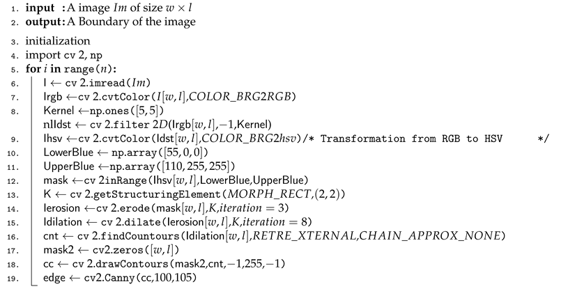
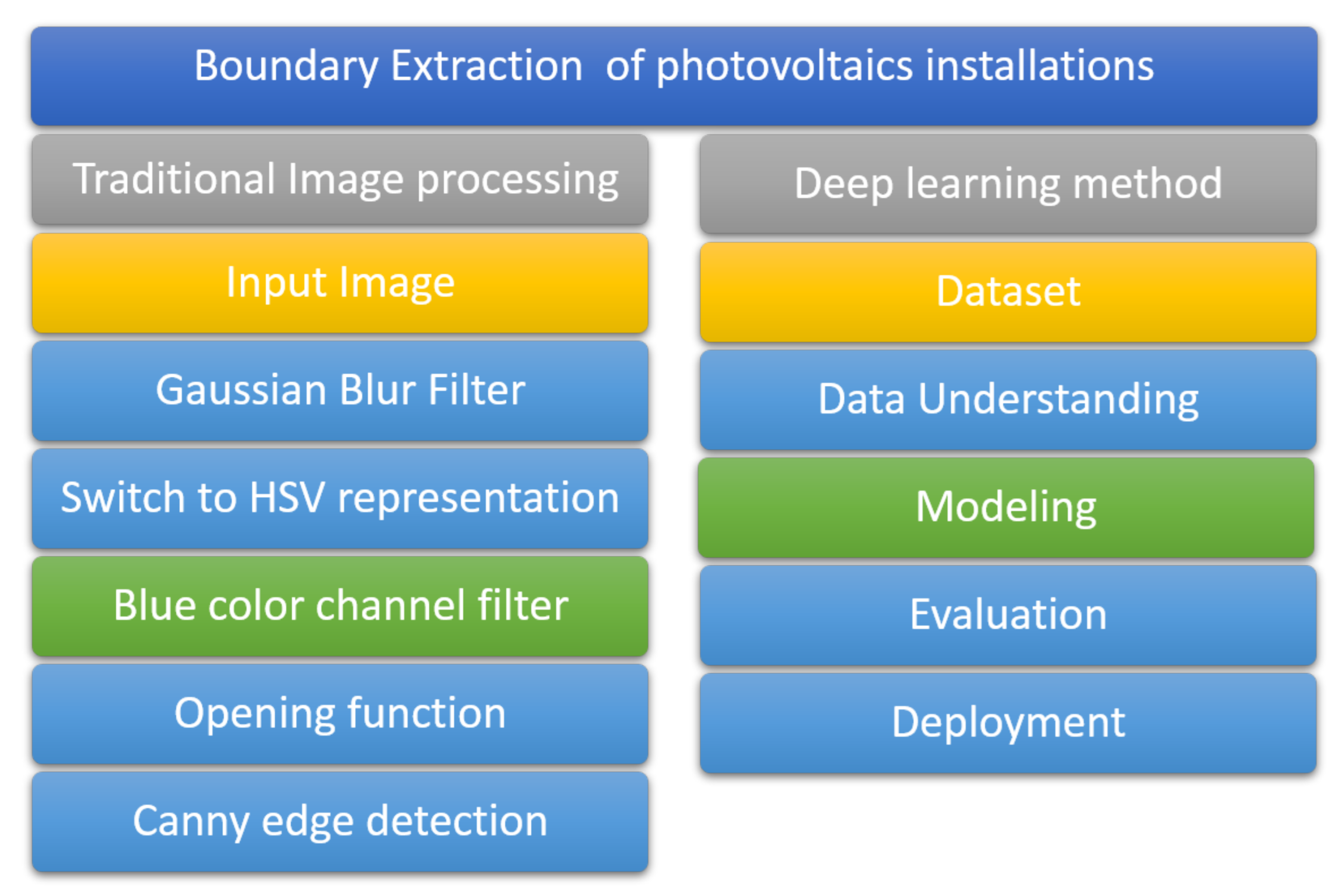
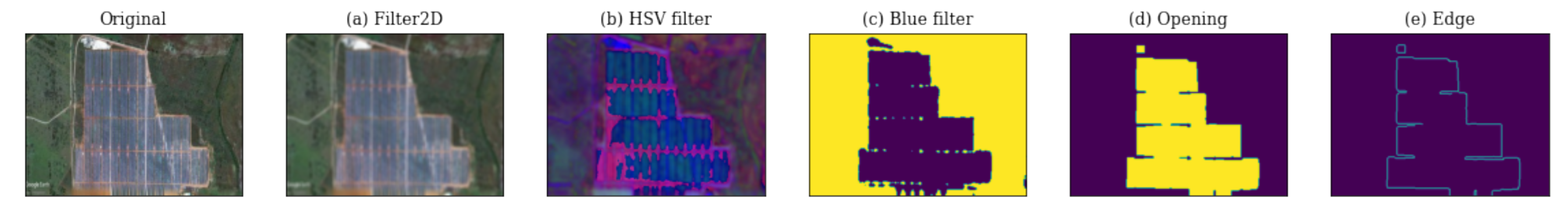
2.3. Traditional Image Processing (TIP)

The process to obtain the boundary pixels of a target can be achieved by means of traditional image processing techniques with functions that extract, increase, filter, and detect the features of an image and obtain its segmentation [27,32]. The main stages were used to remove the borders of PV plants out of an image, as shown in Figure 1 [10]. In the first stage, the original image was filtered using “filter2D” function from OpenCV, that is a convolution filter with 5 × 5 averaging filter kernel, as shown at Algorithm 1. This filter is compound with various Low-Pass Filters (LPF) and High-Pass Filters (HPF). LPF helps in removing noise, blurring images. HPF filters help in finding edges in images.

In the second stage, the filtered image is transformed into the HSV (hue, saturation, and value) representation. The transformation lessens reflection caused by environmental light during aerial image collection. Furthermore, this transformation helps in the color-based segmentation required in the next stages.

In the third stage, each channel was processed separately to extract the area of the PV plants. This was achieved by applying thresholding operations on the HSV image. To extract the PV blue color out of the image, the HSV range limits for thresholding where determined: from $(50,0,0)$ to $(110,255,255)$. Thresholding was implementing using the inRange function of OpenCV.

At the fourth stage, two morphological operators were applied: the “erode” and “dilate” functions. Together these operations helps to reduce noise and to better define the boundaries of the PV devices, the application of erosion followed by dilation is also known as opening operation. Erosion and dilation requires an structuring element (also known as kernel) to be applied to the images. In this case, a rectangular kernel of 2 × 2 pixels (MORPH_RECT,$(2,2)$) was used for both operations. Lines 13, 14 and 15 from Algorithm 1 show the creation of the structuring element and the successive use of the erode and dilate functions.

Then, the “findCountours” function was used to help in extracting the contours from the image. The contour can be defined as a curve joining all the continuous points in the boundary of the PV installation. The input parameters for this function are: the image (dilated image from previous stage), the type of contour to be extracted (in this case only the external contours, RETR_EXTERNAL) and the contour approximation method (in this case not approximation, CHAIN_APPROX_NONE). Finally the area was recognized using a multi-stage algorithm to detect a wide range of edges in images, known as the Canny edge detection “Canny” [44].

The pseudo-code of the Traditional Image Processing is shown in Algorithm 1, and was implemented in Python 3 using OpenCV library.

Algorithm 1: TIP algorithms

2.4. Deep Learning

Another approach to ascertain the boundaries of PV plants uses a DL-based technique which consists of several steps:

2.4.1. Data Specifications

The first step is to select the data for training the Neural Networks. The parameters to take into account are: PV Plants in orthophotos and aerial images with the respective masks for each image [11].

2.4.2. Data Understanding

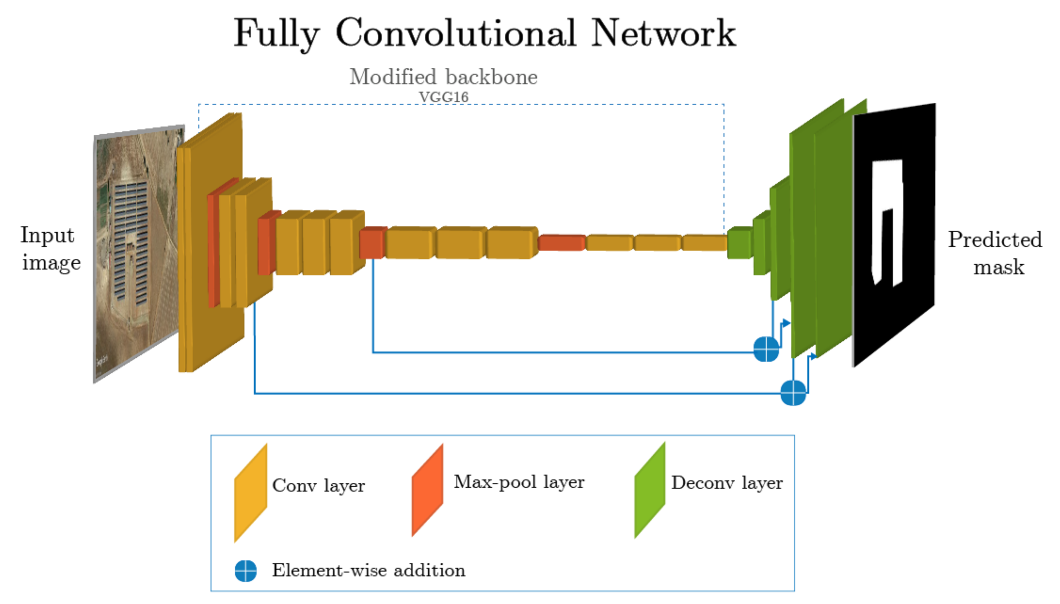
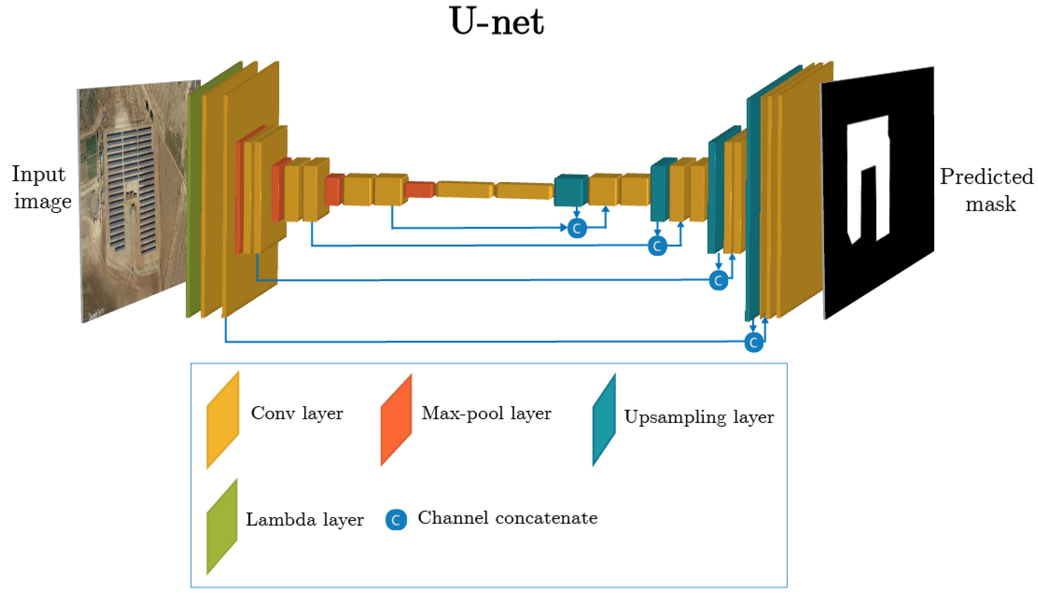
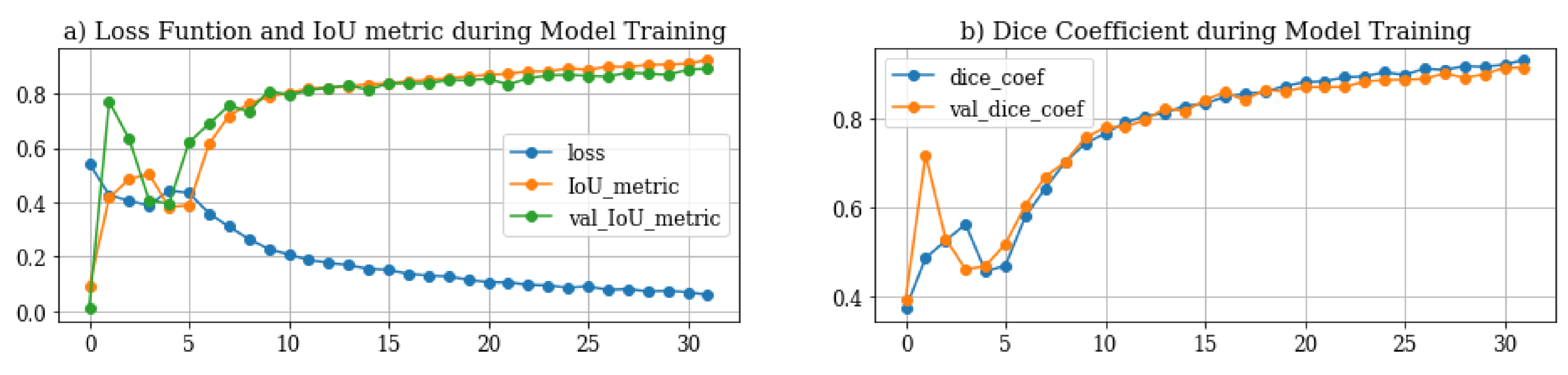
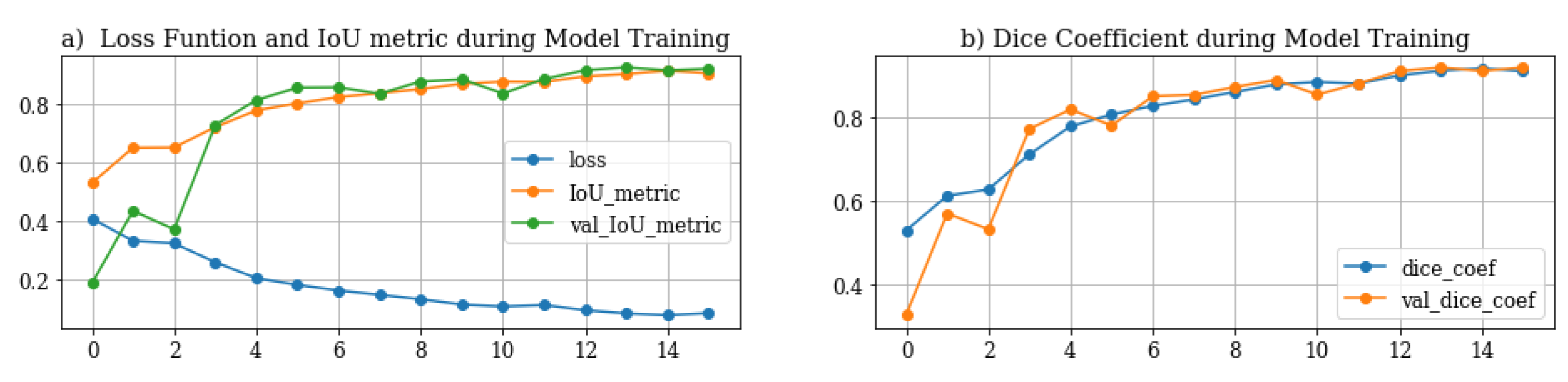
The data preparation phase can be subdivided, into at least four steps. The first step is data selection inside the dataset. The second step involves correcting the individual data, which are assumed to be noisy, apparently incorrect, or absent. The third step involves resizing the data as needed. Finally, most of the available implementations assume that the data are given in a single table, so if the data are in several tables, they must be parsed together in a single one [45].

2.4.3. Modeling

In the literature, the semantic segmentation task has many existing models that can be selected for the desired task. In this work, two methods based on deep learning have been selected, taking into account the following criteria: the most competent for the type of task, the amount of data to be processed, the execution time, and the ease of implementation to predict each label for each pixel. The methods were selected according to [11,46,47,48,49]. The FCN model was the first one selected, which was proposed by [33] and used by [11]. The network architecture is delineated in Figure 2. The second one is the U-Net model, first proposed by [38] and selected for this project. The network architecture is illustrated in Figure 3.

(a). Fully Convolutional Network (FCN) model: This model has two blocks. The first block is a series of 13 layers in order to create a modified version of a VGG16 backbone Figure 2, which was introduced for the first time by [50]. The VGG16 backbone has 16 convolutional layers and its creators belong to the team “Visual Geometry Group”, hence its name VGG16. The backbone is the network that takes the image as input and extracts the feature map upon which the rest of the network is based. The second block consists of a series of deconvolutional layers that simply reverses the forward and backward passes of convolution. The last layer uses a softmax function to predict the probability of the category as shown in Figure 2. As a result, the input of FCN model is an RGB image, and the output is the predicted mask of the PV plants. For more details, read [33]. The parameters for the training process were depicted in

Table 1. Summary of the FCN and U-net model parameters for the training process.

Activation (Last Layers)	Activation (Inner Layers)	Optimizer	Loss Function	Metrics	Epoch	Batch Size
Sigmoid	Relu	RMS	Binary_cross	N/A	150	1
Sigmoid	Elu	Adam	Binary_cross	IoU,F1 score	15	8

.

(b). The U-net network model: This model has two blocks: a decreasing path and an increasing path, respectively, which gives it the u-shaped architecture or horizontal hourglass shape [51]. The decreasing path is a typical convolutional network that consists of repeated application of convolutions, each followed by a rectified linear unit (ReLU) and a max-pooling operation. During the decrease, the spatial information is reduced whereas feature information is increased. The increasing pathway combines the feature and spatial information through a sequence of upsampling layers followed by two layers of transposed convolution for each step [38,52], as illustrated in Figure 3. The parameters for the training process were depicted in Table 1. Its architecture is shown in

Table 2. Architecture of the U-net.

Layer (Type)	Output Shape	Parameters
Input Layer	$(None,240,320,3)$	0
Lambda	$(None,240,320,3)$	0
Conv2D	$(None,240,320,16)$	448
Dropout	$(None,240,320,16)$	0
Conv2D	$(None,240,320,16)$	2320
MaxPooling2D	$(None,120,160,16)$	0
Conv2D	$(None,120,160,32)$	4640
Dropout	$(None,120,160,32)$	0
Conv2D	$(None,120,160,32)$	9248
MaxPooling2D	$(None,60,80,32)$	0
Conv2D	$(None,60,80,64)$	18,496
Dropout	$(None,60,80,64)$	0
Conv2D	$(None,60,80,64)$	36,928
MaxPooling2D	$(None,30,40,64)$	0
Conv2D	$(None,30,40,128)$	73,856
Dropout	$(None,30,40,128)$	0
Conv2D	$(None,30,40,128)$	147,584
MaxPooling2D	$(None,15,20,128)$	0
Conv2D	$(None,15,20,256)$	295,168
Dropout	$(None,15,20,256)$	0
Conv2D	$(None,15,20,256)$	590,080
Conv2D_Transpose	$(None,30,40,128)$	131,200
Concatenate	$(None,30,40,128)$	73,856
Conv2D	$(None,30,40,128)$	295,040
Dropout	$(None,30,40,128)$	0
Conv2D	$(None,30,40,128)$	147,584
Conv2D_Transpose	$(None,60,80,64)$	32,832
Concatenate	$(None,60,80,128)$	0
Conv2D	$(None,60,80,64)$	73,792
Dropout	$(None,60,80,64)$	0
Conv2D	$(None,60,80,64)$	36,928
Conv2D_Transpose	$(None,120,160,32$	8224
Concatenate	$(None,120,160,64)$	0
Conv2D	$(None,120,160,32)$	18,464
Dropout	$(None,120,160,32)$	0
Conv2D	$(None,120,160,32)$	9248
Conv2D_Transpose	$(None,240,320,16)$	2064
Concatenate	$(None,240,320,32)$	0
Conv2D	$(None,240,320,16)$	4624
Dropout	$(None,240,320,16)$	0
Conv2D	$(None,240,320,16)$	2320
Conv2D	$(None,240,320,1)$	17

. The platform used for FCN and Unet models by this work was Tensorflow with Keras backend [53]. The U-net model had never been used for this kind of application so far.

The FCN and U-net models additionally have a binary cross-entropy function ($H_p$) to calculate the loss in the process of training the neuronal network [54]. As the problem at hand is a semantic segmentation task, Equation (1) is used. This function examines each pixel and compares the binary-predicted values vector with the binary-encoded target vector.

$$H_p\left(q\right)=-\frac{1}{N}\sum _{i=1}^N{y}_i·\log \left(p\left(y_i\right)\right)+(1-y_i)·\log (1-p\left(y_i\right))$$

(1)

where y is the label of each pixel, it takes the value of 1 for the PV plants area and 0 to indicate other areas or elements, and $p\left(y\right)$ is the probability of the pixel belonging to the PV plants area for all N points. The Adam optimization function is used to optimize the models [55]. Because semantic segmentation is the task at hand, it is essential to implement metrics to ensure the model performs well.

2.4.4. Metrics

The metrics evaluate the similarities between the predicted mask (N) and the original mask (S). Such similarity assessment can be performed by considering spatial overlapping information, that is, by computing the true positives (TP), false positives (FP) and false negatives (FN) given by $TP=\left|N\cap S\right|$, $FP=\left|N\setminus S\right|$, and $FN=\left|S\setminus N\right|$, respectively.

There are three standard metrics commonly employed to evaluate the effectiveness of the proposed semantic segmentation technique [29,48,49,56]. The three metrics, namely, pixel accuracy (Acc), region Intersection over Union ($IoU$), and Dice Coefficient ($DC$).

Pixel accuracy is the ratio of correctly classified PV plants pixels to the total number of PV plants pixels in the original mask image [57], which can be mathematically represented as Equation (2).

$$Accuracy=\frac{TP}{TP+FN}$$

(2)

The $IoU$ metric (the Jaccard index) is defined by Equation (3). This equation is a ratio between the intersection of the predicted mask N, and the original mask S and the union of both. More details can be found in [58].

$$IoU(N,S)=\frac{|N\cap S|}{|N\cup S|}=\frac{TP}{TP+FP+FN}$$

(3)

The $DC$ metric [56,58,59] is expressed as Equation (4). This equation divides the intersection of the predicted mask N, and the original mask S times two by the sum of N and S.

$$DC(N,S)=\frac{2.|N\cap S|}{\left|N\right|+\left|S\right|}=\frac{2.TP}{2.TP+FP+FN}$$

(4)

To validate the results of the techniques described above, the FCN and U-net models were trained and their performance was evaluated by validating and testing samples of the Amir dataset [43]. The next section describes such results and compares the models in detail.

3. Results and Discussion

3.1. Database Specification

For this work, the DeepSolar [60], Google Sun-Roof [61], OpenPV [62], and Amir’s databases were accessed [43]. Only the last database met the established parameters. It contained PV plants in orthophotos and aerial images with their respective masks. Furthermore, the PV plants images were from different countries around the world. Therefore, the ”Amir” dataset was selected.

3.2. Results with TIP Technique

The results obtained in this work were compared with the results obtained in previous investigations where the TIP and the deep learning techniques were used alongside the FCN model [11].

The stages to obtain the results are shown in Figure 4. In the First Stage, a 2D filter was applied, depicted in Figure 4a. In the second stage, the filtered image is transformed into the HSV representation, Figure 4b. In the third stage, the blue color was filtered out, Figure 4c. At the fourth stage, the opening function was used, as seen in Figure 4d. Finally, the area was recognized using the canny method illustrated in Figure 4e. The results were satisfactory and can be modified depending on the environment.

The results are shown in

Table 3. Comparison between three techniques.

Parameter	TIP Method	FCN Model Amir [11]	U-Net Proposed
Metrics	N/A	N/A	$IoU$, F1 scor
Acc train	N/A	97.99%	97.07%
Acc test	N/A	94.16%	95.44%
$IoU$ metric	N/A	94.13%	93.57%
Dice coef metric	N/A	95.10%	94.03%
val $IoU$ metric	N/A	90.91%	93.51%
val Dice coef	N/A	92.96%	94.44%
test $IoU$ metric	71.62%	87.47%	90.42%
test Dice coef metric	71.62%	89.61%	91.42%

. The TIP technique was obtained by randomly selecting images out of the test dataset, then applying the functions described in the methodology section (Section 2), and finally comparing the mask obtained with the original mask. The $IoU$ metric obtained was $71.62$% and the $DC$ was $71.62$%.

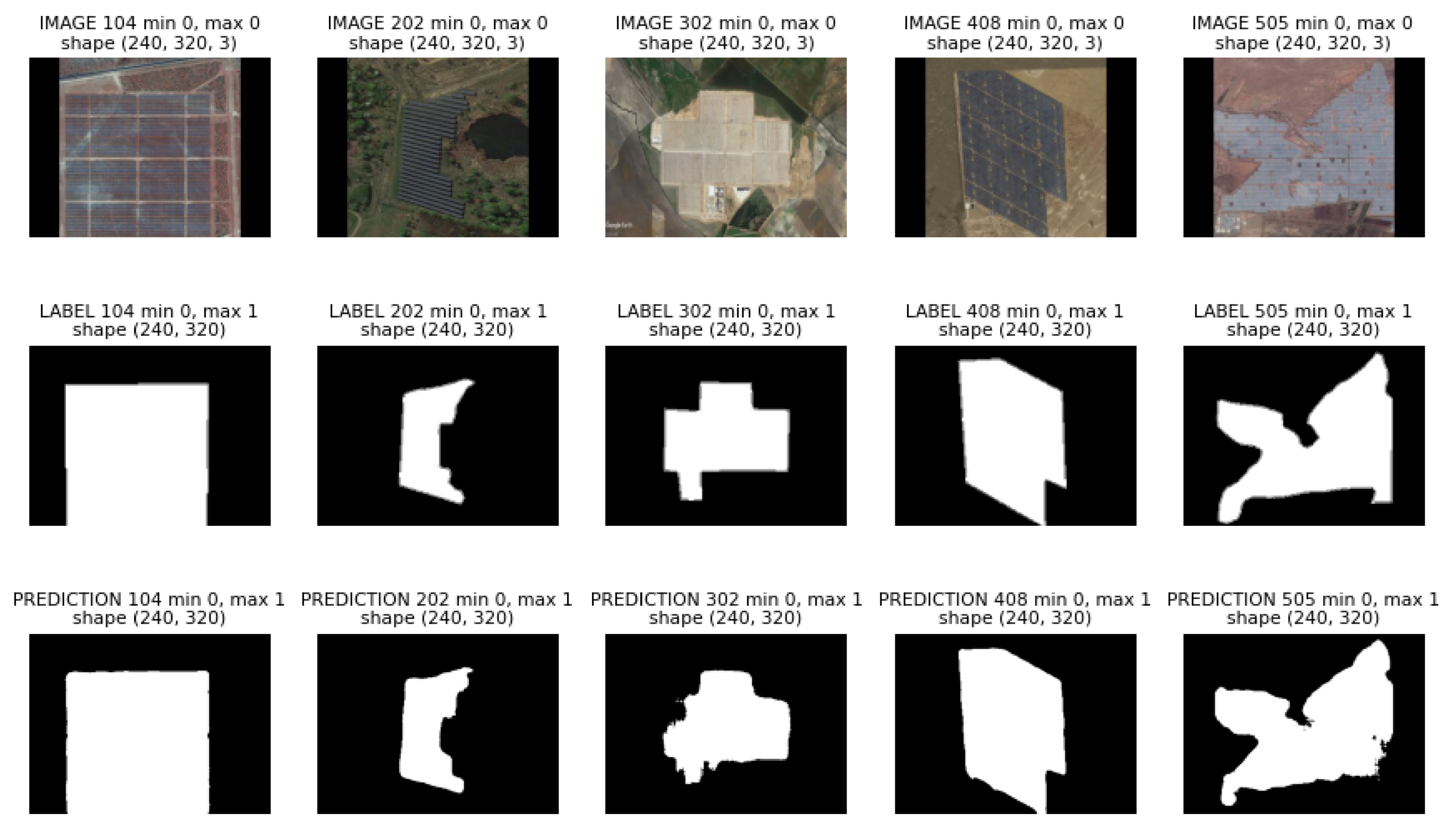
3.3. Results with DL-Based Techniques

The training data consisted of 2864 aerial images selected at random: 90% of the training dataset in the Amir database. The validation data were the remaining 10% of the same training dataset. Figure 5a shows the loss function and $IoU$ metric of the FCN model during the training and validation process. The general trend of the two curves is consistent, showing that the network converges rapidly and is stable at iteration 30, and the loss value tends to $0.04$%. Figure 5b shows the $DC$ metric of the model during the training and validation stage. The general trend of the two curves is consistent at iteration 30.

On the other hand, using the same metrics, the U-net model proposed in this work shows a better performance. Figure 6a shows the loss function and $IoU$ metric of the model during the training and validation stage. The common trend of the two curves shows the network converges quickly and is stable at iteration 16, and the loss value tends to $0.03$%. Figure 6b shows the $DC$ metric of the model all along the training and validation phase. The prevalent trend of the two curves is consistent and in iteration 16.

In the evaluation stage, 716 images were used along with the trained FCN model for PV plant detection. Some relevant results are shown in Figure 7. In this figure, the columns correspond to different PV plants. The first row contains the original images; the second row, the original masks; and, the third one, the predicted masks. The images used were taken in deserted regions and vegetation zones. The FCN model detects the PV plants in vegetation zones with some false positives. As an example, the second and third predictions of Figure 7 identify a lake and vegetation as part of the PV plants. In deserted regions, PV plants are detected more precisely. Although these images have very high precision, their predicted shape does not fully correspond to the original mask. Hence, it was necessary to review the performance metrics of the algorithm [63].

The segmentation results in the evaluation stage, using the same 716 images and the trained U-Net model, are shown in Figure 8. The arrangement is the same as in the previous Figure 7. It is noteworthy that this model correctly segments the photovoltaic plant while the other model does not achieve this result, as can be seen in the second and third predictions in Figure 8.

Afterwards, the trained model tested 716 samples. Table 3 shows the results and comparison among the TIP technique, the U-net proposed model and the FCN model used by [11], which was replicated in this study. The FCN and the proposed U-net models were compared. The accuracies obtained for the FCN model in the stages of training and testing were $97.99$% and $94.16$% respectively [11]. For U-Net proposed, the accuracy obtained in the stages of training and testing were $97.07$% and $95.44$%, respectively. Both results can be seen in Table 3.

To compare the FCN model proposed by Amir [11], and the U-net model proposed in this work, the two most used metrics in semantic segmentation problems were used. The FCN model was implemented with the standard $IoU$ metric, whose result for the training stage was $94.13$%,and the validation stage was $90.91$% and for test stage was $87.47\%$. The $DC$ metric of the validation $92.96$% and test $89.61$% which deviates a little from the training $95.10$%. However, using the same metrics the U-net model proposed in this work shows a better performance. The $IoU$ metric obtained was $93.57$% in the training stage, $93.51$% in the validation stage, and $91.42$% in the test stage. The $DC$ metric of the validation $94.44$% was almost the same as that of the training $94.03$% which deviates a little from the test $91.42$%. Table 3 shows these results. Due to this, a difference was found between the FCN and U-net model for the first metric of $2.95$% and for the second metric used of $1.81$% difference was calculated. All files and logs from the experiments are available at GitHub in [64].

3.4. Discussion

The U-net model proposed reconstructs the segmented image and protects the original image shape characteristics by storing the grouping indices of the max-pooling layer, a process that is not done in the FCN model.

The training and testing accuracy is the percentage of pixels in the image that are classified correctly and cannot be taken as indicators of how similar the predicted PV plants and the original mask are [65]. For the purpose of comparing the similarity in the results, the $IoU$ metric was used. This metric varies from 0 to 1 (0–100%) with 0 meaning no similarity and 1 meaning total similarity between original and predicted masks [63].

The U-net model proposed in this work aimed to obtain a value closer to 1 in the $IoU$ metric. The iteration times show the model used is faster and therefore reliable for the training and processing stages obtaining results virtually in real time [66]. The $DC$ is the other metric used in this work. This metric also ranges from 0 to 1, with 1 signifying the greatest similarity between the predicted and original masks [63]. Both metrics were used to determine if the U-net model was better than the FCN model in the validation and test stages. The values of the $IoU$ and Dice metrics in Table 3 showed the U-net model had a better performance when compared to the FCN model. This work was implemented with VGG16 as an encoder because it was the encoder used by Amir [11], which is a comparison work, but in future work, it is possible to use other encoders like ResNet, AlexNet, etc. [37].

Finally, the results obtained with the TIP and FCN model agree with the results obtained by other authors [11,13]. The authors mentioned they did not use the standard metrics for these kinds of problems and the bias in the results were expected. On the contrary, this work did take these metrics into account and found satisfactory results. The U-net network increased the processing speed, veracity in the segmentation process, and the overall performance of the model.

4. Conclusions

This work used three techniques, namely, the TIP technique, the DL-based FCN and U-net models. This work applied the U-net model to PV plants. All the models were used for the extraction of the PV plants boundaries out of an image. As a consequence, the TIP technique can be very precise but requires constant adjustment depending on the image, whereas the FCN and U-net network models are more useful when it comes to unknown PV plants.

The U-net network model is novel for this kind of problem. It allows greater processing speeds and performance when predicting the area of PV plants, also better features. The results obtained open the door for further investigation of this model in this problem.

The U-net technique turned out to be satisfactory compared to the TIP technique and the FCN model used in previous studies. The values obtained in the implemented metrics guarantee that the areas predicted for the PV plants are similar to the real ones. The results also help to predict possible false positives, such as lakes in the vicinity of photovoltaic plants. The relevant features of an object can be obtained using this technique while using the FCN technique is not possible.

References

1. Donovan, C.W. Renewable Energy Finance: Funding the Future of Energy; World Scientific Publishing Co. Pte. Ltd.: London, UK, 2020. [Google Scholar]
2. Philipps, S.; Warmuth, W. Photovoltaics Report Fraunhofer Institute for Solar Energy Systems. In ISE with Support of PSE GmbH November 14th; Fraunhofer ISE: Freiburg, Germany, 2019. [Google Scholar]
3. Jamil, W.J.; Rahman, H.A.; Shaari, S.; Salam, Z. Performance degradation of photovoltaic power system: Review on mitigation methods. Renew. Sustain. Energy Rev. 2017, 67, 876–891. [Google Scholar] [CrossRef]
4. Kaplani, E. PV cell and module degradation, detection and diagnostics. In Renewable Energy in the Service of Mankind Vol II; Springer: Cham, Switzerland, 2016; pp. 393–402. [Google Scholar]
5. Di Lorenzo, G.; Araneo, R.; Mitolo, M.; Niccolai, A.; Grimaccia, F. Review of O&M Practices in PV Plants: Failures, Solutions, Remote Control, and Monitoring Tools. IEEE J. Photovolt. 2020, 10, 914–926. [Google Scholar]
6. Guerrero-Liquet, G.C.; Oviedo-Casado, S.; Sánchez-Lozano, J.; García-Cascales, M.S.; Prior, J.; Urbina, A. Determination of the Optimal Size of Photovoltaic Systems by Using Multi-Criteria Decision-Making Methods. Sustainability 2018, 10, 4594. [Google Scholar] [CrossRef] [Green Version]
7. Grimaccia, F.; Leva, S.; Niccolai, A.; Cantoro, G. Assessment of PV plant monitoring system by means of unmanned aerial vehicles. In Proceedings of the 2018 IEEE International Conference on Environment and Electrical Engineering and 2018 IEEE Industrial and Commercial Power Systems Europe (EEEIC/I&CPS Europe), Palermo, Italy, 12–15 June 2018; pp. 1–6. [Google Scholar]
8. Shen, K.; Qiu, Q.; Wu, Q.; Lin, Z.; Wu, Y. Research on the Development Status of Photovoltaic Panel Cleaning Equipment Based on Patent Analysis. In Proceedings of the 2019 3rd International Conference on Robotics and Automation Sciences (ICRAS), Wuhan, China, 1–3 June 2019; pp. 20–27. [Google Scholar]
9. Azaiz, R. Flying Robot for Processing and Cleaning Smooth, Curved and Modular Surfaces. U.S. Patent 15/118.849, 2 March 2017. [Google Scholar]
10. Grimaccia, F.; Aghaei, M.; Mussetta, M.; Leva, S.; Quater, P.B. Planning for PV plant performance monitoring by means of unmanned aerial systems (UAS). Int. J. Energy Environ. Eng. 2015, 6, 47–54. [Google Scholar] [CrossRef] [Green Version]
11. Sizkouhi, A.M.M.; Aghaei, M.; Esmailifar, S.M.; Mohammadi, M.R.; Grimaccia, F. Automatic boundary extraction of large-scale photovoltaic plants using a fully convolutional network on aerial imagery. IEEE J. Photovolt. 2020, 10, 1061–1067. [Google Scholar] [CrossRef]
12. Leva, S.; Aghaei, M.; Grimaccia, F. PV power plant inspection by UAS: Correlation between altitude and detection of defects on PV modules. In Proceedings of the 2015 IEEE 15th International Conference on Environment and Electrical Engineering (EEEIC), Rome, Italy, 10–13 June 2015; pp. 1921–1926. [Google Scholar]
13. Aghaei, M.; Dolara, A.; Leva, S.; Grimaccia, F. Image resolution and defects detection in PV inspection by unmanned technologies. In Proceedings of the 2016 IEEE Power and Energy Society General Meeting (PESGM), Boston, MA, USA, 17–21 July 2016; pp. 1–5. [Google Scholar]
14. Grimaccia, F.; Leva, S.; Dolara, A.; Aghaei, M. Survey on PV modules’ common faults after an O&M flight extensive campaign over different plants in Italy. IEEE J. Photovolt. 2017, 7, 810–816. [Google Scholar]
15. Quater, P.B.; Grimaccia, F.; Leva, S.; Mussetta, M.; Aghaei, M. Light Unmanned Aerial Vehicles (UAVs) for cooperative inspection of PV plants. IEEE J. Photovolt. 2014, 4, 1107–1113. [Google Scholar] [CrossRef] [Green Version]
16. Oliveira, A.K.V.; Aghaei, M.; Madukanya, U.E.; Rüther, R. Fault inspection by aerial infrared thermography in a pv plant after a meteorological tsunami. Rev. Bras. Energ. Sol. 2019, 10, 17–25. [Google Scholar]
17. De Oliveira, A.K.V.; Amstad, D.; Madukanya, U.E.; Do Nascimento, L.R.; Aghaei, M.; Rüther, R. Aerial infrared thermography of a CdTe utility-scale PV power plant. In Proceedings of the 2019 IEEE 46th Photovoltaic Specialists Conference (PVSC), Chicago, IL, USA, 16–21 June 2019; pp. 1335–1340. [Google Scholar]
18. AGHAEI, M. Novel Methods in Control and Monitoring of Photovoltaic Systems. Ph.D. Thesis, Politecnico di Milano, Milan, Italy, 2016. [Google Scholar]
19. Li, X.; Li, W.; Yang, Q.; Yan, W.; Zomaya, A.Y. An Unmanned Inspection System for Multiple Defects Detection in Photovoltaic Plants. IEEE J. Photovolt. 2019, 10, 568–576. [Google Scholar] [CrossRef]
20. Aghaei, M.; Leva, S.; Grimaccia, F. PV power plant inspection by image mosaicing techniques for IR real-time images. In Proceedings of the 2016 IEEE 43rd Photovoltaic Specialists Conference (PVSC), Portland, OR, USA, 5–10 June 2016; pp. 3100–3105. [Google Scholar]
21. Aghaei, M.; Gandelli, A.; Grimaccia, F.; Leva, S.; Zich, R.E. IR real-time analyses for PV system monitoring by digital image processing techniques. In Proceedings of the 2015 International Conference on Event-Based Control, Communication and Signal Processing (EBCCSP), Krakow, Poland, 17–19 June 2015; pp. 1–6. [Google Scholar]
22. Menéndez, O.; Guamán, R.; Pérez, M.; Auat Cheein, F. Photovoltaic modules diagnosis using artificial vision techniques for artifact minimization. Energies 2018, 11, 1688. [Google Scholar] [CrossRef] [Green Version]
23. López-Fernández, L.; Lagüela, S.; Fernández, J.; González-Aguilera, D. Automatic evaluation of photovoltaic power stations from high-density RGB-T 3D point clouds. Remote Sens. 2017, 9, 631. [Google Scholar] [CrossRef] [Green Version]
24. Niccolai, A.; Grimaccia, F.; Leva, S. Advanced asset management tools in photovoltaic plant monitoring: UAV-based digital mapping. Energies 2019, 12, 4736. [Google Scholar] [CrossRef] [Green Version]
25. Tsanakas, J.A.; Chrysostomou, D.; Botsaris, P.N.; Gasteratos, A. Fault diagnosis of photovoltaic modules through image processing and Canny edge detection on field thermographic measurements. Int. J. Sustain. Energy 2015, 34, 351–372. [Google Scholar] [CrossRef]
26. Yao, Y.Y.; Hu, Y.T. Recognition and location of solar panels based on machine vision. In Proceedings of the 2017 2nd Asia-Pacific Conference on Intelligent Robot Systems (ACIRS), Wuhan, China, 16–18 June 2017; pp. 7–12. [Google Scholar]
27. Sizkouhi, A.M.M.; Esmailifar, S.M.; Aghaei, M.; De Oliveira, A.K.V.; Rüther, R. Autonomous path planning by unmanned aerial vehicle (UAV) for precise monitoring of large-scale PV plants. In Proceedings of the 2019 IEEE 46th Photovoltaic Specialists Conference (PVSC), Chicago, IL, USA, 16–21 June 2019; pp. 1398–1402. [Google Scholar]
28. Rodriguez-Esparza, E.; Zanella-Calzada, L.A.; Oliva, D.; Heidari, A.A.; Zaldivar, D.; Pérez-Cisneros, M.; Foong, L.K. An efficient Harris hawks-inspired image segmentation method. Expert Syst. Appl. 2020, 155, 113428. [Google Scholar] [CrossRef]
29. Garcia-Garcia, A.; Orts-Escolano, S.; Oprea, S.; Villena-Martinez, V.; Martinez-Gonzalez, P.; Garcia-Rodriguez, J. A survey on deep learning techniques for image and video semantic segmentation. Appl. Soft Comput. 2018, 70, 41–65. [Google Scholar] [CrossRef]
30. Pal, N.R.; Pal, S.K. A review on image segmentation techniques. Pattern Recognit. 1993, 26, 1277–1294. [Google Scholar] [CrossRef]
31. Hoeser, T.; Kuenzer, C. Object detection and image segmentation with deep learning on Earth observation data: A review-part I: Evolution and recent trends. Remote Sens. 2020, 12, 1667. [Google Scholar] [CrossRef]
32. Henry, C.; Poudel, S.; Lee, S.W.; Jeong, H. Automatic detection system of deteriorated PV modules using drone with thermal camera. Appl. Sci. 2020, 10, 3802. [Google Scholar] [CrossRef]
33. Long, J.; Shelhamer, E.; Darrell, T. Fully convolutional networks for semantic segmentation. In Proceedings of the IEEE Conference on Computer Vision and Pattern Recognition, Boston, MA, USA, 7–12 June 2015; pp. 3431–3440. [Google Scholar]
34. Puttemans, S.; Van Ranst, W.; Goedemé, T. Detection of photovoltaic installations in RGB aerial imaging: A comparative study. In Proceedings of the GEOBIA 2016 Proceedings, Enschede, The Netherlands, 14–16 September 2016. [Google Scholar]
35. Karoui, M.S.; Benhalouche, F.Z.; Deville, Y.; Djerriri, K.; Briottet, X.; Houet, T.; Weber, C. Partial linear NMF-based unmixing methods for detection and area estimation of photovoltaic panels in urban hyperspectral remote sensing data. Remote Sens. 2019, 11, 2164. [Google Scholar] [CrossRef] [Green Version]
36. Bhatnagar, S.; Gill, L.; Ghosh, B. Drone Image Segmentation Using Machine and Deep Learning for Mapping Raised Bog Vegetation Communities. Remote Sens. 2020, 12, 2602. [Google Scholar] [CrossRef]
37. Sothe, C.; Almeida, C.M.D.; Schimalski, M.B.; Liesenberg, V.; Rosa, L.E.C.L.; Castro, J.D.B.; Feitosa, R.Q. A comparison of machine and deep-learning algorithms applied to multisource data for a subtropical forest area classification. Int. J. Remote Sens. 2020, 41, 1943–1969. [Google Scholar] [CrossRef]
38. Ronneberger, O.; Fischer, P.; Brox, T. U-net: Convolutional networks for biomedical image segmentation. In Proceedings of the International Conference on Medical Image Computing and Computer-Assisted Intervention, Munich, Germany, 5–9 October 2015; Springer: Cham, Switzerland, 2015; pp. 234–241. [Google Scholar]
39. Ren, M.; Zemel, R.S. End-to-end instance segmentation with recurrent attention. In Proceedings of the IEEE Conference on Computer Vision and Pattern Recognition, Honolulu, HI, USA, 21–26 July 2017; pp. 6656–6664. [Google Scholar]
40. McCollum, B.T. Analyzing GPS Accuracy through the Implementation of Low-Cost Cots Real-Time Kinematic GPS Receivers in Unmanned Aerial Systems; Technical Report; Air Force Institute of Technology Wright-Patterson AFB OH Wright-Patterson: Fort Belvoir, VA, USA, 2017. [Google Scholar]
41. Mission Planner Home–Mission Planner Documentation. Available online: https://ardupilot.org/planner/ (accessed on 2 May 2021).
42. QGroundControl, Intuitive and Powerful Ground Control Station for the MAVLink Protocol. Available online: http://qgroundcontrol.com/ (accessed on 15 April 2021).
43. Sizkouhi, M.; Aghaei, M.; Esmailifar, S.M. Aerial Imagery of PV Plants for Boundary Detection. 2020. Available online: https://ieee-dataport.org/documents/aerial-imagery-pv-plants-boundary-detection (accessed on 14 December 2020).
44. Canny, J. A Computational Approach to Edge Detection. IEEE Trans. Pattern Anal. Mach. Intell. 1986, PAMI-8, 679–698. [Google Scholar] [CrossRef]
45. Berthold, M.R.; Borgelt, C.; Höppner, F.; Klawonn, F.; Silipo, R. Data preparation. In Guide to Intelligent Data Science; Springer: Cham, Switzerland, 2020; pp. 127–156. [Google Scholar]
46. Abdollahi, A.; Pradhan, B.; Alamri, A.M. An ensemble architecture of deep convolutional Segnet and Unet networks for building semantic segmentation from high-resolution aerial images. Geocarto Int. 2020, 1–16. [Google Scholar] [CrossRef]
47. Minaee, S.; Boykov, Y.Y.; Porikli, F.; Plaza, A.J.; Kehtarnavaz, N.; Terzopoulos, D. Image segmentation using deep learning: A survey. IEEE Trans. Pattern Anal. Mach. Intell. 2021. [Google Scholar] [CrossRef]
48. Hao, S.; Zhou, Y.; Guo, Y. A brief survey on semantic segmentation with deep learning. Neurocomputing 2020, 406, 302–321. [Google Scholar] [CrossRef]
49. Lateef, F.; Ruichek, Y. Survey on semantic segmentation using deep learning techniques. Neurocomputing 2019, 338, 321–348. [Google Scholar] [CrossRef]
50. Simonyan, K.; Zisserman, A. Very deep convolutional networks for large-scale image recognition. arXiv 2014, arXiv:1409.1556. [Google Scholar]
51. Cao, M.; Zou, Y.; Yang, D.; Liu, C. GISCA: Gradient-inductive segmentation network with contextual attention for scene text detection. IEEE Access 2019, 7, 62805–62816. [Google Scholar] [CrossRef]
52. Shibuya, N.; Up-Sampling with Transposed Convolution. Towards Data Science. 2017. Available online: https://naokishibuya.medium.com/up-sampling-with-transposed-convolution-9ae4f2df52d0 (accessed on 24 February 2021).
53. Abadi, M.; Agarwal, A.; Barham, P.; Brevdo, E.; Chen, Z.; Citro, C.; Corrado, G.S.; Davis, A.; Dean, J.; Devin, M.; et al. TensorFlow: Large-Scale Machine Learning on Heterogeneous Systems. 2015. Available online: https://www.tensorflow.org/ (accessed on 1 May 2021).
54. Alain, G.; Bengio, Y. What regularized auto-encoders learn from the data-generating distribution. J. Mach. Learn. Res. 2014, 15, 3563–3593. [Google Scholar]
55. Yi, D.; Ahn, J.; Ji, S. An Effective Optimization Method for Machine Learning Based on ADAM. Appl. Sci. 2020, 10, 1073. [Google Scholar] [CrossRef] [Green Version]
56. Rizzi, M.; Guaragnella, C. Skin Lesion Segmentation Using Image Bit-Plane Multilayer Approach. Appl. Sci. 2020, 10, 3045. [Google Scholar] [CrossRef]
57. Talal, M.; Panthakkan, A.; Mukhtar, H.; Mansoor, W.; Almansoori, S.; Al Ahmad, H. Detection of water-bodies using semantic segmentation. In Proceedings of the 2018 International Conference on Signal Processing and Information Security (ICSPIS), Dubai, United Arab Emirates, 7–8 November 2018; pp. 1–4. [Google Scholar]
58. Powers, D.M. Evaluation: From precision, recall and F-measure to ROC, informedness, markedness and correlation. arXiv 2020, arXiv:2010.16061. [Google Scholar]
59. Alalwan, N.; Abozeid, A.; ElHabshy, A.A.; Alzahrani, A. Efficient 3D Deep Learning Model for Medical Image Semantic Segmentation. Alex. Eng. J. 2021, 60, 1231–1239. [Google Scholar] [CrossRef]
60. Yu, J.; Wang, Z.; Majumdar, A.; Rajagopal, R. DeepSolar: A machine learning framework to efficiently construct a solar deployment database in the United States. Joule 2018, 2, 2605–2617. [Google Scholar] [CrossRef] [Green Version]
61. Elkin, C. Sun Roof Project. 2015. Available online: http://google.com/get/sunroof (accessed on 14 December 2020).
62. NREL. Open PV Project; U.S. Department of Energy’s Solar Energy Technologies Office: Denver, CO, USA, 2018; Available online: https://www.nrel.gov/pv/open-pv-project.html (accessed on 14 December 2020).
63. Costa, M.G.F.; Campos, J.P.M.; e Aquino, G.D.A.; de Albuquerque Pereira, W.C.; Costa Filho, C.F.F. Evaluating the performance of convolutional neural networks with direct acyclic graph architectures in automatic segmentation of breast lesion in US images. BMC Med. Imaging 2019, 19, 85. [Google Scholar] [CrossRef] [PubMed]
64. Perez, A. 2021. Available online: https://github.com/andresperez86/BoundaryExtractionPhotovoltaicPlants (accessed on 26 May 2021).
65. Qiongyan, L.; Cai, J.; Berger, B.; Okamoto, M.; Miklavcic, S.J. Detecting spikes of wheat plants using neural networks with Laws texture energy. Plant Methods 2017, 13, 83. [Google Scholar] [CrossRef] [Green Version]
66. Ling, Z.; Zhang, D.; Qiu, R.C.; Jin, Z.; Zhang, Y.; He, X.; Liu, H. An accurate and real-time method of self-blast glass insulator location based on faster R-CNN and U-net with aerial images. CSEE J. Power Energy Syst. 2019, 5, 474–482. [Google Scholar]
Figure 1. Steps of boundary extraction by image analysis with two techniques.
Applsci 11 06524 g001
Figure 2. FCN model.
Applsci 11 06524 g002
Figure 3. U-net Model.
Applsci 11 06524 g003
Figure 4. Steps of boundary extraction by TIP.
Applsci 11 06524 g004
Figure 5. Performance and metrics of the FCN model using the training and validation sets.
Applsci 11 06524 g005
Figure 6. Performance and metrics of the U-net model obtained using the training and validation sets.
Applsci 11 06524 g006
Figure 7. Evaluation with test data FCN Model.
Applsci 11 06524 g007
Figure 8. Evaluation with test data U-net Model.
Applsci 11 06524 g008